SlideShare ist ein Scribd-Unternehmen logo
1 von 49
©www.vom-mathelehrer.de	
	
Analysis – Übungsblatt 1
Grundwissen – lineare und quadratische Funktionen - Lösung
1.
2. 3.
4. 5.
a) f(x) = −3x + 4 m = −3 ; t = 4
b) f(x) = x − 2 m =1 ; t = −2
c) f(x) = −2 m = 0 ; t = −2
d) f(x) =
3
5
x +
3
2
m =
3
5
; t =
3
2
m =
Δy
Δx
=
yQ
− yP
xQ
− xP
=
5 − 7
4 − 2
=
−2
2
= −1
7 = −1⋅ 2+ t
t = 9
g: y = −x +9
a) y =1
b) m = −1
1= −1⋅(−5) + t
t = −4
y = −x − 4
c) x = −5
m = tan(30°) =
3
3
−0,5 =
3
3
⋅3+ t
t = −0,5 − 3
y =
3
3
x −0,5 − 3
mg
⋅mf
= −1
mg
= −
1
2
−2,5 = −
1
2
⋅ 4+ t
t = −0,5 = −
1
2
g: y = −
1
2
x −
1
2
©www.vom-mathelehrer.de	
	
6.
a) Normalform entspricht hier Scheitelpunktform
S(0 | −2)
Y(0 | −2)
f(x) = x2
− 2 = (x − 2)(x + 2)
N1
( 2 | 0) ; N2
(− 2 | 0)
b) f(x) = x2
− 4x +3 = x2
− 4x + 4 −1
= (x − 2)2
−1
S(2 | −1)
Y(0 | 3)
x1,2
=
4± 16 −12
2
=
4± 2
2
(Alternative : Vieta)
x1
=1 ; x2
= 3
N1
(1| 0) ; N2
(3 | 0)
c) f(x) = −2x2
− 4x +3
= −2[x2
+ 2x −1,5]
= −2[x2
+ 2x +1− 2,5]
= −2[(x +1)2
− 2,5]
= −2(x +1)2
+5
S(−1| 5)
Y(0 | 3)
x1,2
=
4± 16+ 24
−4
=
4± 2 10
−4
N1
−
2+ 10
2
| 0
⎛
⎝
⎜
⎜
⎞
⎠
⎟
⎟; N2
−2+ 10
2
| 0
⎛
⎝
⎜
⎜
⎞
⎠
⎟
⎟
d) f(x) = x2
+ 2x = x(x + 2) = x2
+ 2x +1−1= (x +1)1
−1
S(−1| −1)
Y(0 | 0)
N1
(0 | 0) ; N2
(−2 | 0)
Alternative :
x −Koordinate von S liegt wegen Symmetrie zwischen Nst.
S(−1| y) y durch einsetzen bestimmen.
"
#
$
$
$
%
&
'
'
'
©www.vom-mathelehrer.de	
	
7.
8.
Wenn man die gegebenen Punkte in die Gleichung y = ax2
+ bx + c einsetzt, ergibt sich das
Gleichungssystem:
Daraus ergibt sich a = -1, b = -6 und c = -7, also y = - x2
- 6x - 7.
Scheitelpunktform: y = - (x+3)2
+ 2 , also S(-3/2).
Nullstellen:
e) f(x) = 2(x −3)(x + 2)
N1
(−2 | 0) ; N2
(3 | 0)
Y(0 | −12)
S(0,5 | y); f(0,5) = −12,5
f(x) = 2(x −0,5)2
−12,5
f(x) = a(x − d)2
+ e
f(x) = a(x +0,5)2
−0,5 = a⋅0,52
a = −2
f(x) = −2(x +0,5)2
I. −
1
4
=
81
4
a −
9
2
b + c
II. 1= 4a − 2b+ c
III. − 2= a − b+ c
x1
=−3 − 2 und x2
= −3+ 2.
©www.vom-mathelehrer.de	
	
Analysis – Übungsblatt 2
Grundwissen - ganzrationale Funktionen - Lösung
1.
a) f(x) = x(x+2)2
eine einfache NSt bei 0 mit VzW
und eine doppelte bei – 2 ohne VzW
b) f(x) = x(x2
+ 2x + 3) eine einfache NSt bei 0 mit VzW
c) f(x) = (x + 1)(x3
+ 9x2
+ 26x + 24) = (x + 1)(x + 2)(x2
+ 7x + 12) =
= (x + 1)(x + 2)(x + 3)(x + 4) vier einfache NSt bei -1, -2, -3 und -4 mit VzW
2.
.	
Da die höchste Potenz einen geraden Exponenten besitzt und einen negativen
Koeffizienten verläuft der zugehörige Graph von „links unten“ nach „rechts unten“.
.
Da die höchste Potenz einen ungeraden Exponenten besitzt und den positiven
Koeffizienten +1, verläuft der zugehörige Graph von „links unten“ nach „rechts oben“.
3.


4.	
	
	
5. A(1|0) , B(3|0) , C(-1|0)
f(x) = (x2
−3x)(x − x2
) = x3
− x4
−3x2
+3x3
= −x4
+ 4x3
−3x2
4
x-
h(x) = −34
+ x3
−5x2
= x3
−5x2
−81
x3
f(x) = a x − x1( ) x − x2( ) x − x3( ) und f(0) = 2
f(x) = (x −1)(x +1)(x − 2) = x3
− 2x2
− x + 2
(x4
− 5x3
− 30x2
+ 40x + 64) :(x +1) = x3
− 6x2
− 24x + 64
−(x4
+ x3
)
− 6x3
− 30x2
−(−6x3
− 6x2
)
− 24x2
+ 40x
−(−24x2
− 24x)
64x + 64
−(−64x + 64)
0
©www.vom-mathelehrer.de	
	
6.
a)
-> Der Graph von f ist punktsymmetrisch bezüglich des Koordinatenursprungs.
b)
=> Da für den Graphen von f weder noch gilt,
liegt keine Achsensymmetrie bezüglich der y-Achse und auch keine Punktsymmetrie
bezüglich des Koordinatenursprungs vor.
7.
a) bedeutet, dass der Graph von f an der y-Achse gespiegelt wird. Der Faktor 2
bewirkt, dass zusätzlich noch eine Streckung in y-Richtung (von der x-Achse aus) um den
Faktor 2.
b) bewirkt, dass der Graph von f in x-Richtung (von der y-Achse aus) mit dem Faktor 2
gestreckt wird. Der Summand +2 bedeutet, dass der Graph zusätzlich um 2 Einheiten nach
oben verschoben wird.
8.
a)
b)
c)
d)
e)
f(−x) = 3(−x)3
(2−(−x)2
) = −3x3
(2− x2
) = −f(x)
f(−x) = (−x + 2)2
(−x)3
= −(2− x)2
x3
f(−x) = f(x) f(−x) = −f(x)
f(−x)
f(
1
2
x)
lim
x→+∞
5 −
1
x2
→+∞
!
→0
!
⎛
⎝
⎜
⎜
⎜
⎜
⎜
⎞
⎠
⎟
⎟
⎟
⎟
⎟
= 5 ; lim
x→+∞
5 −
1
x2
→+∞
!
→0
!
⎛
⎝
⎜
⎜
⎜
⎜
⎜
⎞
⎠
⎟
⎟
⎟
⎟
⎟
= 5
lim
x→+∞
2−x
= 0 ; lim
x→−∞
2−x
= +∞
lim
x→+∞
(2x3
+ x − 3) = +∞ ; lim
x→−∞
(2x3
+ x − 3) = −∞
lim
x→+∞
(2x3
− x − 3) = +∞ ; lim
x→−∞
(2x3
− x − 3) = +∞
lim
x→+∞
(x − 2x3
−3) = lim
x→+∞
(−2x3
+ x −3) = −∞
lim
x→−∞
(x − 2x3
−3) = lim
x→−∞
(−2x3
+ x −3) = +∞
©www.vom-mathelehrer.de	
	
Analysis – Übungsblatt 3
Gebrochenrationale Funktionen 1- Lösung
1.
a)
b)
c)
d)
e)
f)
Definitionsmenge : x − 2 = 0 ↔ x = 2 → D = IR  {2}
Nullstelle : 5x + 4 = 0 ↔ x = −
4
5
Definitionsmenge : x + 4 = 0 ↔ x = −4 → D = IR  {−4}
Nullstellen: 2x2
+1= 0 ↔ x2
= −
1
2
→ keine Nst., da keine Zahl mit sich selbst multipliziert −
1
2
ergibt.
Definitionsmenge : x2
− 4 = 0 ↔ x2
= 4 ↔ x = ±2 → D = IR  {−2; 2}
Nullstellen: −2x2
− 3x + 9 = 0
x1,2
=
3± 9+ 72
−6
=
3± 9
−6
; x1
= −2 (keine Nst, da nicht in Definitionsmenge enthalten)
x2
=1
f(x) =
x2
− 4
x + 2
=
(x + 2)(x − 2)
x + 2
= x − 2
Definitionsmenge : x + 2 = 0 ↔ x = −2 → D = IR  {−2}
Nullstellen: x2
− 4 = 0 ↔(x + 2)(x − 2) = 0
x1
= −2 (keine Nst., da nicht in der Definitionsmenge enthalten)
x2
= 2
f(x) =
3x2
− 3
x −1
=
3(x2
−1)
x −1
=
3(x −1)(x +1)
x −1
= 3(x +1)
Definitionsmenge : D = IR  {1}
Nullstelle : x = −1
f(x) =
6x2
− 4x − 42
x −3
Definitionsmenge : D = IR  {3}
Nullstellen: x1,2
=
4± 16+1008
12
=
4±32
12
x1
= 3 (keine Nst.) x2
= −
7
3
→ f(x) = 6x +14 (Definitionsmenge bleibt erhalten; Polynomdivision)
©www.vom-mathelehrer.de	
	
2.
3.
f(x) =
1
x − 2
+3 =
1
x − 2
+
3(x − 2)
x − 2
=
1+3x − 6
x − 2
=
3x −5
x − 2
f(x) =
1
x +1
−
1
x +3
=
x +3
(x +1)(x +3)
−
x +1
(x +1)(x +3)
=
(x +3) −(x +1)
(x +1)(x +3)
=
2
(x +1)(x +3)
(1. Term)
=
2
x2
+3x + x +3
=
2
x2
+ 4x +3
(2. Term)
=
2
x2
+ 4x + 4 −1
=
2
(x + 2)2
−1
=
1
1
2
[(x + 2)2
−1]
=
1
0,5(x + 2)2
−0,5
(3. Term)
Evtl. einf acher : 3. Term ausmultiplizieren und zu 2. Term umformen!!!
©www.vom-mathelehrer.de	
	
Analysis – Übungsblatt 4
Gebrochenrationale Funktionen 2 - Lösung
1.
a)
b)
c)
d)
e)
f)
f(x) =
5x + 4
x − 2
; D = IR  {2}
lim
x→2
>
5x + 4
→14!"#
x − 2
+0
!
⎛
⎝
⎜
⎜
⎜
⎜
⎞
⎠
⎟
⎟
⎟
⎟
= +∞ ; lim
x→2
<
5x + 4
→14!"#
x − 2
−0
!
⎛
⎝
⎜
⎜
⎜
⎜
⎞
⎠
⎟
⎟
⎟
⎟
= −∞ ; Polstelle mit VZW
f(x) =
2x2
+1
x + 4
; D = IR  {−4}
lim
x→−4
>
2x2
+1
33!"#
x + 4
+0
!
⎛
⎝
⎜
⎜
⎜
⎜
⎞
⎠
⎟
⎟
⎟
⎟
= +∞ ; lim
x→−4
<
2x2
+1
33!"#
x + 4
−0
!
⎛
⎝
⎜
⎜
⎜
⎜
⎞
⎠
⎟
⎟
⎟
⎟
= −∞ ; Polstelle mit VZW
f(x) =
−2x2
−3x +9
x2
− 4
; D = IR  {−2;2}
lim
x→−2
>
−2x2
−3x +9
→7! "## $##
x2
− 4
→−0
%&'
⎛
⎝
⎜
⎜
⎜
⎜
⎞
⎠
⎟
⎟
⎟
⎟
= −∞ ; lim
x→−2
<
−2x2
−3x +9
→7! "## $##
x2
− 4
→−0
%&'
⎛
⎝
⎜
⎜
⎜
⎜
⎞
⎠
⎟
⎟
⎟
⎟
= +∞ ; Polstelle mit VZW
lim
x→2
>
−2x2
−3x +9
→−5! "## $##
x2
− 4
→+0
%&'
⎛
⎝
⎜
⎜
⎜
⎜
⎞
⎠
⎟
⎟
⎟
⎟
= −∞ ; lim
x→−2
<
−2x2
−3x +9
→−5! "## $##
x2
− 4
→−0
%&'
⎛
⎝
⎜
⎜
⎜
⎜
⎞
⎠
⎟
⎟
⎟
⎟
= +∞ ; Polstelle mit VZW
f(x) =
x2
− 4
x + 2
=
(x + 2)(x − 2)
x + 2
= x − 2 ; D = IR  {−2}
lim
x→2
>
x − 2( )= 0 ; lim
x→2
<
x − 2( )= 0 ; hebbare Definitionslücke
f(x) =
3x2
−3
x −1
=
3(x2
−1)
x −1
=
3(x −1)(x +1)
x −1
= 3(x +1) ; D = IR  {1}
lim
x→1
>
3(x +1)( )= 6 ; lim
x→1
<
3(x +1)( )= 6 ; hebbare Definitionslücke
f(x) =
6x2
− 4x − 42
x −3
= 6x +14 ; D = IR  {3}
lim
x→3
>
6x +14( )= 32 ; lim
x→−3
<
6x +14( )= 32 ; hebbare Definitionslücke
www.vom-mathelehrer.de	
	
Analysis – Übungsblatt 5
Gebrochen-rationale Funktionen 3 - Lösung
1.
a)
b)
c)
f(x) =
5x + 4
x − 2
; D = IR  {2}
lim
x→±∞
5x + 4
x − 2
⎛
⎝
⎜
⎞
⎠
⎟ = 5 ("z = n" → Vergleiche Leitkoeffizienten)
Alternative : lim
x→±∞
5x + 4
x − 2
⎛
⎝
⎜
⎞
⎠
⎟ = lim
x→±∞
x 5+
4
x
⎛
⎝
⎜
⎞
⎠
⎟
x 1−
2
x
⎛
⎝
⎜
⎞
⎠
⎟
⎛
⎝
⎜
⎜
⎜
⎜
⎞
⎠
⎟
⎟
⎟
⎟
= lim
x→±∞
5+
4
x
→±0!
1−
2
x
→±0
"
⎛
⎝
⎜
⎜
⎜
⎜
⎜
⎜
⎞
⎠
⎟
⎟
⎟
⎟
⎟
⎟
= 5
Sprichen Sie mit Ihrem Mathelehrer, was er sehen möchte!
senkr : x = 2
waagr : y = 5
f(x) =
2x2
+1
x + 4
= 2x −8+
33
x + 4
; D = IR  {−4}
lim
x→−∞
2x −8+
33
x + 4
→0
!
⎛
⎝
⎜
⎜
⎜
⎞
⎠
⎟
⎟
⎟
= −∞ ; lim
x→+∞
2x −8+
33
x + 4
→0
!
⎛
⎝
⎜
⎜
⎜
⎞
⎠
⎟
⎟
⎟
= +∞
senkr.: x = −4
schräg: y = 2x −8 ("z = n+1")
f(x) =
−2x2
−3x +9
x2
− 4
; D = IR  {−2;2}
lim
x→−∞
−2x2
−3x +9
x2
− 4
⎛
⎝
⎜⎜
⎞
⎠
⎟⎟ = −2 ; lim
x→+∞
−2x2
−3x +9
x2
− 4
⎛
⎝
⎜⎜
⎞
⎠
⎟⎟ = −2 ("z = n" → Vergleiche Leitkoeffizienten)
senkr : x = −2 ; x = 2
waagr : y = −2
www.vom-mathelehrer.de	
	
d)
e)
f)
2.
f(x) =
x2
− 4
x + 2
=
(x + 2)(x − 2)
x + 2
= x − 2 ; D = IR  {−2}
lim
x→−∞
>
x − 2( )= −∞ ; lim
x→+∞
x − 2( )= +∞
f(x) =
3x2
−3
x −1
=
3(x2
−1)
x −1
=
3(x −1)(x +1)
x −1
= 3(x +1) ; D = IR  {1}
lim
x→−∞
3(x +1)( )= −∞ ; lim
x→+∞
3(x +1)( )= +∞
f(x) =
6x2
− 4x − 42
x −3
= 6x +14 ; D = IR  {3}
lim
x→−∞
6x +14( )= −∞ ; lim
x→+∞
6x +14( )= +∞
f(x) =
20x
x2
− 25
=
20x
(x −5)(x +5)
Betrachte die Nennernullstellen für die Definitionsmenge!
→ D = IR  {−5; 5}
Symmetrie : f(−x) =
20(−x)
(−x)2
− 25
=
−20x
x2
− 25
= −
20x
x2
− 25
= f(x)
→ Punktsymmetrie bzgl. (0 | 0)
senkr.: x = −5 ; x = 5
waagr.: y = 0 ("z < n")
www.vom-mathelehrer.de	
	
3.
I: Steigung passt nicht
II: passt nicht, das Polstelle mit VZW im Graph dargestellt ist, die Funktionsgleichung jedoch
eine Nullstelle ersten Grades besitzt.
4.
0 =
1
2
⋅(−1) −1+
a
(−1−1)2
0 = −1,5+
a
4
a = 6
a) D = IR  {1}
SX
(−3 | 0)
SY
(0 | −9)
b)x + 7+
16
x −1
=
x(x −1)
x −1
+
7(x −1)
x −1
+
16
x −1
=
x2
− x + 7x − 7+16
x −1
=
x2
+ 6x +9
x −1
=
(x +3)2
x −1
= f(x)
oder bei f(x) Zähler ausmultiplizieren und Polynomdivision durchführen.
g ist schräge Asymptote von Gf
.
www.vom-mathelehrer.de	
	
Analysis – Übungsblatt 6
Differenzenquotient – mittlere Änderungsrate
Differentialquotient – lokale Änderungsrate - Lösung
1.
2a)
											
b)
	
	
3.
	
	
4a)
	
	
A(0 | 730) ; B(21000 | 2962)
Durchschn. Steigung: m =
Δy
Δx
=
yB
− yA
xB
− xA
=
2969 − 730
21000 −0
=
2239
21000
≈ 0,107
Steigungswinkel: m = tan(α) =
Gegenkathete
Ankathete
=
Δy
Δx
=
yB
− yA
xB
− xA
α = tan−1 2239
21000
⎛
⎝
⎜
⎞
⎠
⎟ ≈ 6,09°
I1
:
f(b) − f(a)
b − a
=
5⋅52
−5⋅ 22
5 − 2
=
355
3
I2
:
f(b) − f(a)
b − a
=
5⋅ 42
−5⋅ 22
4 − 2
= 30
I3
:
f(b) − f(a)
b − a
=
5⋅32
−5⋅ 22
3 − 2
= 25
f '(x0
) = lim
x→x0
f(x) − f(x0
)
x − x0
= lim
x→2
f(x) − f(2)
x − 2
= lim
x→2
5x2
− 5⋅ 22
x − 2
= lim
x→2
5(x2
− 4)
x − 2
= lim
x→2
5(x + 2)(x − 2)
x − 2
=
= lim
x→2
5(x + 2) = 5⋅(2+ 2) = 20 = f '(2)
f '(x0
) = lim
x→x0
f(x) − f(x0
)
x − x0
= lim
x→−1
f(x) − f(−1)
x −(−1)
= lim
x→2
1
5
x2
−
1
2
x + 2−(
1
5
⋅(−1)2
−
1
2
⋅(−1) + 2)
x +1
=
= lim
x→−1
1
5
x2
−
1
2
x + 2−
1
5
−
1
2
− 2
x +1
= lim
x→−1
1
5
x2
−
1
2
x −
7
10
x +1
= lim
x→−1
x −
7
2
⎛
⎝
⎜
⎞
⎠
⎟ x +1( )
x +1
= lim
x→−1
x −
7
2
⎛
⎝
⎜
⎞
⎠
⎟ = −
9
2
NR : x1,2
=
1
2
±
1
4
+ 4⋅
1
5
⋅
7
10
2
5
=
1
2
±
81
100
2
5
x1
=
7
2
; x2
= −1
⎛
⎝
⎜
⎜
⎜
⎜
⎜
⎜
⎜
⎞
⎠
⎟
⎟
⎟
⎟
⎟
⎟
⎟
n(t) = 3t2
− 60t + 500
m =
n(2) −n(0)
2− 0
=
3⋅ 22
− 60⋅ 2+ 500 − 500
2
= −54
mittlere Änderungsrate : −54
1
h
I":
f(b) − f(a)
b − a
=
5 ∙ 5- − 5 ∙ 2-
5 − 2
= 35
www.vom-mathelehrer.de	
	
5)
f(x) = 2x ⋅e−0,5x2
mS
=
f(0,5) − f(−0,5)
0,5 −(−0,5)
=
e−0,53
−(−e−0,53
)
1
= 2e−0,53
≈ 1,76
f '(x) = 2⋅e−0,5x2
+ 2x ⋅e−0,5x2
⋅(−x) = 2e−0,5x2
(1− x2
)
mT
= f '(0) = 2e0
(1−0) = 2
mT
−mS
mT
≈ 0,12 =12%
www.vom-mathelehrer.de	
	
Analysis – Übungsblatt 7
Tangente –- Ableitung – Stammfunktion - Lösung
1)
2)
3)
4) g
f(x) = 5x2
f '(x) =10x
m = f '(2) = 20
y = mx + t
20 = 20⋅ 2+ t ↔ t = −20
y = 20x − 20
f(x) =
1
5
x2
−
1
2
x + 2
f '(x) =
2
5
x −
1
2
m = f '(−1) = −
9
10
y = mx + t
27
10
= −
9
10
⋅(−1) + t ↔ t =1,8
y = −
9
10
x +1,8
F(x) = x2
− 2x
F'(x0
) = lim
x→x0
x2
− 2x − x0
2
− 2x0( )
x − x0
= lim
x→x0
x2
− x0
2
−(2x − 2x0
)
x − x0
= lim
x→x0
(x − x0
)(x + x0
)
x − x0
− lim
x→x0
2(x − x0
)
x − x0
= lim
x→x0
x + x0( )− 2 = 2x0
− 2 = f(x0
)
Definitionsmengen vergleichen!!!
→ F ist Stammfunktion zu f
www.vom-mathelehrer.de	
	
5)
	
lim
t→t0
3t2
− 60t +500 −(3t0
2
− 60t0
+500)
t − t0
= lim
t→t0
3t2
− 60t −3t0
2
+ 60t0
t − t0
= lim
t→t0
3t2
−3t0
2
−(60t − 60t0
)
t − t0
= lim
t→t0
3t2
−3t0
2
0
t − t0
− lim
t→t0
60t − 60t0
t − t0
= lim
t→t0
3(t − t0
)(t + t0
)
t − t0
− lim
t→t0
60(t − t0
)
t − t0
= lim
t→t0
3(t − t0
) − 60 = 6t0
− 60
f '(x) = 6t − 60 (Später ohne Diff '− qu ableiten!!!)
−30 = 6t − 60
6t = 30
t = 5
5 Stunden nach Beginn...
www.vom-mathelehrer.de	
	
Analysis – Übungsblatt 8
Summen- und Faktorregel - Lösung
1)
2)
3)
An diesen Stellen besitzt der Graph eine Tangente, die parallel zur x-Achse verläuft.
4)
5)
	
f(x) = x3
− x2
+ x +1 ; f '(x) = 3x2
− 2x +1
g(x) =
1
3
x3
−
1
2
x2
+ x +1 ; g'(x) = x2
− x +1
h(x) =18 − x3
+ 3x2
; h'(x) = −3x2
+ 6x
i(x) = −3 ; i'(x) = 0
j(x) = 4x(x −1)2
= 4x(x2
− 2x +1) = 4x3
− 8x2
+ 4x ; j'(x) =12x2
−16x + 4
k(x) =
1
x
−1= x−1
−1 ; k'(x) = −x−2
= −
1
x2
l(x) =
5
x2
+
5x
2
= 5x−2
+
5
2
x ; l'(x) = −10x−3
+ 2,5 = −
10
x3
+ 2,5
f(x) = x3
− 2x2
; f '(x) = 3x2
− 4x
f(2) = 0
f '(2) = 4
y = mx + t
0 = 4⋅ 2+ t ↔ t = −8
y = 4x −8
f(x) = x3
− 6x2
+11x − 6
f '(x) = 3x2
−12x +11
f ''(x) = 6x −12
www.vom-mathelehrer.de	
	
Analysis – Übungsblatt 9
Produkt- und Quotientenregel - Lösung
1)
2a)
Definitionslücken: egal
Nullstellen: I
Asymptoten: III
SP y-Achse: II
b)
3a)
b)
Ist die Kettenregel bekannt, kann diese Aufgabe „geschickter“ gelöst werden.
4)
f '(x) =1⋅(x2
+ x +1) +(x −1)(2x +1) = x2
+ x +1+ 2x2
+ x − 2x −1= 3x2
g'(x) =
(x − 2)⋅1− x ⋅1
(x − 2)2
=
−2
(x − 2)2
h'(x) =
(2x −3)⋅(2x −1) −(x2
− x)⋅ 2
(2x −3)2
=
2x2
− 6x +3
(2x −3)2
i'(x) = 0
j(x) = 4x(x −1)2
= 4x(x2
− 2x +1) = 4x3
− 8x2
+ 4x ; j'(x) =12x2
−16x + 4
k(x) =
1
x
−1= x−1
−1 ; k'(x) = −x−2
= −
1
x2
l(x) =
5
x2
+
5x
2
= 5x−2
+
5
2
x ; l'(x) = −10x−3
+ 2,5 = −
10
x3
+ 2,5
f '(x) =
x2
+ 4x +13
(x + 2)2
I: 4x = 0 ↔ x = 0
II: senkr : x = −1
III: "z < n"
f(x) =
4x
(x +1)2
=
4x
x2
+ 2x +1
f '(x) =
(x2
+ 2x +1)⋅ 4 − 4x ⋅(2x + 2)
(x +1)4
=
4(x +1)2
−8x(x +1)
(x +1)4
=
(x +1)[4(x +1) −8x]
(x +1)4
=
4x + 4 −8x
(x +1)3
=
−4x + 4
(x +1)3
D = IR  {−
5
4
}
f '(x) =
(4x +5)⋅ 2−(2x +3)⋅ 4
(4x +5)2
=
4x +10 −8x −12
(4x +5)2
= −
2
(4x +5)2
www.vom-mathelehrer.de	
	
Analysis – Übungsblatt 10
Monotonie und Extrempunkte - Lösung
1)
	
	
f '(x) = 3x2
− x +1
f '(x)=
!
0
3x2
− x +1= 0
x1,2
=
1± 1−12
6
; keine Nullstelle der ersten Ableitung
→ keine waagrechte Tangete an Gf
→ kein Extremum
Monotonie : f '(x) > 0 für alle x ∈ ID
f ist streng monoton wachsend.
g'(x) =
(x − 2)⋅1− x ⋅1
(x − 2)2
=
−2
(x − 2)2
; Dg
= Dg'
= IR  {2}
g'(x) ≠ 0 ; keine Nullstellen der ersten Ableitung
→ keine waagrechte Tangete an Gf
→ kein Extremum
Monotonie :
x : − − − − − +
2
Def.−L
− − − −− >
f '(x) : < 0 < 0
Gf
fällt fällt
www.vom-mathelehrer.de	
	
h'(x) =
(2x −3)⋅(2x −1) −(x2
− x)⋅ 2
(2x −3)2
=
2x2
− 6x +3
(2x −3)2
; Dh
= Dh'
= IR  {1,5}
h'(x)=
!
0
2x2
− 6x +3 = 0
x1,2
=
6± 36 − 24
4
=
6± 2 3
4
x1
=
3+ 3
2
; x2
=
3 − 3
2
Gf
besitzt waagrechte Tangente; potentielle Extrempunkte( )
Monotonie :
x : − − − − − +
3− 3
2
− − − − − − +
1,5
Def.−L
− − − − − − +
3+ 3
2
− − − − − − >
f '(x) : > 0 < 0 < 0 > 0
Gf
: steigt fällt fällt steigt
HOP TIP
3 − 3
2
|
2− 3
2
⎛
⎝
⎜
⎜
⎞
⎠
⎟
⎟
3+ 3
2
|
2+ 3
2
⎛
⎝
⎜
⎜
⎞
⎠
⎟
⎟
l'(x) = −10x−3
+ 2,5 = −
10
x3
+ 2,5 ; Dl
= Dl'
= IR  {0}
l'(x)=
!
0
−
10
x3
+ 2,5 = 0 ↔
10
x3
= 2,5 ↔ x3
= 4 ↔ x = 43
Monotonie :
x : − − − − − − +
0
Def.−L
− − − − − − +
43
− − − − − − >
f '(x) : > 0 < 0 > 0
Gf
: steigt fällt steigt
TIP
43
| 5,95( )
www.vom-mathelehrer.de	
	
2a)
b)
3)
z.B. lim
x→+∞
1
a
>0
x
→+∞
( x2
→+∞
−1)
⎛
⎝
⎜
⎜
⎞
⎠
⎟
⎟
= +∞
→ Abbildung 2
fa
'(x) =
3
a
⋅ x2
−1
fa
'(x)=
!
0
3
a
⋅ x2
−1= 0 ↔ x2
=
a
3
↔ x1,2
= ±
a
3
x −Koord. des Extrempunkts einsetzen:
3 = ±
a
3
9 =
a
3
↔ a = 27 → f27
(x) =
1
27
x3
− x ; f '27
(x) =
1
9
x2
−1
Pr obe auf Extrempunkt : (da Gf
punktsymm. bzgl. (0 | 0) ist, wird Monotonie für x > 0 untersucht)
x : − − − − −+
3
− − − −− >
f '(x) : < 0 > 0
Gf
fällt steigt
TIP
Ist die zweite Ableitung bekannt :
f ''a
(x) =
6
a
x ; f ''27
(3) =
6
27
⋅3 ≠ 0
⎛
⎝
⎜
⎜⎜
⎞
⎠
⎟
⎟⎟
f '(x) = 4x3
− 6x2
f '(x)=
!
0
4x3
− 6x2
= 0
2x2
(2x −3) = 0
x1
= 0 ; x2
=1,5
Monotonie :
x : − − − − − −+
0
− − − − − − +
1,5
− − − −− >
f '(x) : < 0 < 0 > 0
Gf
: fällt fällt steigt
TEP TIP
aus a) bekannt 1,5 | −1,69( )
www.vom-mathelehrer.de	
Analysis–Übungsblatt11
Kurvendiskussion
-LösungKurvendiskussionrationalerFunktionen
UmbestimmteEigenschaftendesGraphenablesenzukönnen,eignensichunterschiedlicheDarstellungsformendesFunktionsterms:
1.Definitionsmenge
DieDefinitionsmengeistentwederangegeben(z.B.beiAnwendungsbezügen),ansonsten
istdiemaximaleDefinitionsmengefür
-ganz-rationaleFunktionenganzIR.
-gebrochen-rationaleFunktionenganzIRohnegegebenenfallsdie
Nennernullstellen.
2.Symmetrie
AllgemeinerAnsatzzurUntersuchung:
-f(–x)=f(x)
ÞAchsensymmetriezury-Achse
-f(–x)=–f(x)
ÞPunktsymmetriezumUrsprung
Speziellfürganz-rationaleFunktionen:
-nurgeradeExponenten
ÞAchsensymmetrie
-nurungeradeExponenten
ÞPunktsymmetrie
HatdieFunktioneineSymmetrie,kannmansichoftdieHälftederArbeit„sparen“!
f(x)=
x3
x2
−1
=
x3
(x+1)(x−1)
=x+
x
x2
−1
Df
=IR{−1;1}
f(−x)=
(−x)3
(−x)2
−1
=
(−1)3
x3
(−1)2
x2
−1
=−
x3
x2
−1
=−f(x)
→PunktsymmetriezumKoordinatenursprung.
www.vom-mathelehrer.de	
	
3.SchnittpunktmitdenKoordinatenachsen
Schnittpunktmitdery-AchseSy(0/f(0)):f(0)=yo
Schnittpunktmitderx-AchseSx(x0/0):f(x)=0
StrategienbeiderNullstellensuche:
-Ausklammern,wennmöglich,vonxn
Þn-facheNullstellebeixo=0
-ErrateneinerNullstellex1ÞPolynomdivisiondesFunktionstermsdurch(x–x1)
-QuadratischeTermemitLösungsformelauswerten
-LineareGleichungenmitÄquivalenzumformungauflösen
DieVielfachheiteinerNullstelleermöglichteinigeinteressanteSchlussfolgerungen:
-UngeradeVielfachheitÞVorzeichenwechsel(geradeVielfachheitÞkeinVZW)
-DieVielfachheiteinerNullstelleistinderAbleitungumeinsniedriger!
-DieVielfachheitverrätetwasüberdenVerlaufdesGrapheninderUmgebungder
Nullstelle:
oEinfacheNullstelle:SchnittpunktwiebeieinerGeradenmitderx-Achse
oDoppelteNullstelle:Berührpunkt(wiebeiParabel),lokalerExtrempunkt
oDreifacheNullstelle:TerrassenpunktanderNullstelle
f(0)=
03
02
−1
=0
→Sy
(0/0)
f(x)=0
x3
x2
−1
=0⇔x3
=0⇔x=0
dreifacheNullstelle

→Sx
(0/0)
www.vom-mathelehrer.de	
	
4.VerhaltenimUnendlichen
Beiganz-rationalenFunktionenbestimmtderSummandmitdemgrößtenExponentendas
Verhaltenfürf(x).
Fürgebrochen-rationaleFunktionengiltfürdenZählergradzunddenNennergradn
-z<n:x-AchseistwaagrechteAsymptote
-z=n:waagrechteAsymptote
-z=n+1:schrägeAsymptote
-z>n+1:keineAsymptote
ZurBestimmungderAsymptoteneignensich:
•SenkrechteAsymptoten:Nennernullstellen,sofernsiesichnichtgegen
Zählernullstellenkürzenlassen
•WaagrechteAsymptoten:AusklammernundKürzenderhöchstenvorkommenden
Potenz,fallsz<noderz=n
•SchrägeAsymptoten:DurchführungderPolynomdivision,fallsz>n
5.VerhaltenandenDefinitionslücken
(fürgerochen-rationaleFunktionen)
WirdderNenner,jedochnichtderZähler,fürxpnull,sobesitztdieFunktionhiereine
Polstelle.DerGraphbesitzteinesenkrechteAsymptotemitderGleichungx=xp.
HabenZählerundNennergemeinsameNullstellen,sozerlegtmanbeideinLinearfaktoren
undkürzt.DamitkannmanDefinitionslückenbeheben.
lim
x→−∞
x+
x
x2
−1
=lim
x→−∞
x+
x2
⋅
1
x
x2
(1−
1
x2
)
=lim
x→−∞
x
→−∞
+
1
x
→0
1−
1
x2
→0

→0

=−∞
lim
x→+∞
x+
x
x2
−1
=lim
x→+∞
x+
x2
⋅
1
x
x2
(1−
1
x2
)
=lim
x→+∞
x
→+∞
+
1
x
→0
1−
1
x2
→0

→0

=+∞
lim
x→xp
f(x)=±∞
lim
x→
<
−1
x3
→−1
x2
−1
→+0

=−∞lim
x→
<
1
x3
→1
x2
−1
→−0

=−∞
lim
x→
>
−1
x3
→−1
x2
−1
→−0

=+∞lim
x→
>
1
x3
→1
x2
−1
→+0

=+∞
www.vom-mathelehrer.de	
	
6.MonotonieverhaltenundExtrempunkte
DasMonotonieverhaltenbestimmtmananhanddesVorzeichensderAbleitung(Tabelle).
Extrempunkte:AllgemeinerAnsatzzurUntersuchung:f’(x)=0
DieVielfachheitderNullstellevonf´ermöglichtwiederinteressanteSchlussfolgerungen:
-UngeradeVielfachheitÞVZWvonf’ÞlokalerExtrempunkt(HOP,TIP)
-DoppelteNullstellevonf’ÞkeinVZWvonf’ÞTerrassenpunkt(TEP),keinExtrempunkt
	
	
Intervallx<<
x<-1
-1<x<00<x<11<x<<x
Vorzeichen
vonf´
+-----
Monotonie
vonGf
HOPDef.-L.TEPDef.-LTIP
HOP(|f())TEP(0|f(0))TIP(|f())
f'(x)=
x4
−3x2
x4
−2x2
+1
;
f'(x)=0⇔x4
−3x2
=0
x2
(x2
−3)=0;x2
(x+3)(x−3)=0
x1
=0;x2
=−3;x3
=+3
−3−3
3
3
−3−333
www.vom-mathelehrer.de	
	
7.SkizzedesGraphen
AlleInformationenaufdenPunkten1–6werdenverwendetundeswirdanschaulichklar,
obessichbeidenlokalenExtrempunktenauchumglobaleExtremahandelt.Bei
eingeschränkterDefinitionsmengemüssendazunochdieFunktionswerteandenRändern
berechnetwerden.
www.vom-mathelehrer.de	
	
Analysis – Übungsblatt 12
Newton und Umkehrfunktion - Lösung
1)
Die Tangenten an den Graphen in Hoch- bzw. Tiefpunkt sind parallel zur x-Achse. Dadurch
existiert kein Schnittpunkt von Tangente und x-Achse und das Verfahren kann nicht
ausgeführt werden.
ODER:
2)
3)
4)
	
xn+1
= xn
−
f(xn
)
f '(xn
)
Im Extermpunkt gilt f '(xn
) = 0
→ Durch Null darf nicht dividiert werden.
→ Verfahren kann nicht ausgeführt werden.
f−1
x( )=
1
x
Df−1 = IR  {0}
Wf−1 = IR  {0}
f x( )=1+
1
x
y =1+
1
x
↔ y −1=
1
x
↔ x =
1
y −1
f−1
(x) =
1
x −1
Df−1 = IR  {1}
Wf−1 = IR  {0}
y =
2x
1+5x
↔(1+5x)y = 2x ↔ y +5xy = 2x ↔ y = 2x −5xy ↔ y = x(2−5y) ↔ x =
y
2−5y
f−1
x( )=
x
2−5x
Df−1 = IR  {
2
5
}
Wf−1 = IR  {−
1
5
}
www.vom-mathelehrer.de	
	
5) Gf ist achsensymmetrisch bzgl. der Winkelhalbierenden des 1. Und 3. Quadranten.
6) Nicht umkehrbar auf IR, da jede Parallele zur x-Achse mit der Gleichung y=a mit -1≤a≤1
Gf unendlich oft schneidet. Mögliches Intervall I=[0; π]
www.vom-mathelehrer.de	
	
Analysis – Übungsblatt 13
Trigonometrische Funktionen - Lösung
1)
2) z.B.: a=6
3 α) z.B.: a=1; c=1
β) z.B.: a=2; c=0
4) a)k=π
b)
f(x) = sin(x) + cos(x) ; f '(x) = cos(x) − sin(x)
g(x) =
1
2
cos(x) −
1
2
sin(x) ; g'(x) = −
1
2
sin(x) −
1
2
cos(x)
h(x) = 3 ⋅cos(x) ; h'(x) = − 3 ⋅sin(x)
i(x) = − 3 ⋅cos(x) ; i'(x) = 3 ⋅sin(x)
j(x) = x + 3 ⋅sin(x) ; j'(x) =1+ 3 ⋅cos(x)
k(x) =
1
9
x3
⋅cos(x) ; k'(x) =
1
3
x2
⋅cos(x) −
1
9
x3
⋅sin(x) (Produktregel)
y = x +k mit k ≠ 0
z.B.: y = x −1
www.vom-mathelehrer.de	
	
Analysis – Übungsblatt 14
Funktionen mit rationalen Exponenten - Lösung
1)
2a)
b)
3)
f(x) = x = x
1
2
; Df
= IR+
0
; f '(x) =
1
2
x
−
1
2
=
1
2 x
g(x) =
1
x
= x
−
1
2
; Dg
= IR+
; g'(x) = −
1
2
x
−
3
2
= −
1
2x x
= −
x
2x2
h(x) = 3 ⋅ x ; Dh
= IR ; h'(x) = 3
i(x) =
x
x
=
x x
x
= x ; Di
= IR+
; i'(x) =
1
2 x
j(x) = x + x ; Dj
= IR+
0
; j'(x) =1+
1
2 x
k(x) = x ⋅cos(x) ; Dk
= IR+
0
; k'(x) =
1
2 x
⋅cos(x) − x ⋅sin(x)
Definitionsmenge :
4+ x ≥ 0
x ≥ −4
Dg
= [−4; +∞[
SP mit y − Achse :
g(0) = 2⋅ 4+ 0 −1= 3
Sy
(0 | 3)
Von innen nach außen:
x → x + 4 : Verschiebung um 4 Einheiten nach links
x + 4 → 2⋅ x + 4 : Streckung um Faktor 2 in y −Richtung
2⋅ x + 4 → 2⋅ x + 4 −1: Verschiebung um 1 Einheit nach unten
Wertemenge : Wg
= [−1 ; +∞[
www.vom-mathelehrer.de	
	
x2
−b ≥ 0
x2
≥ b
| x |≥ b
x ≥ b oder −x ≥ b ↔ x ≤ − b
Dg
= IR]− b ; b[
b = 2 → b = 4
www.vom-mathelehrer.de	
	
Analysis – Übungsblatt 15
Kettenregel - Lösung
1)
2a)
f '(x) = 2(3x − 4)3 = 6(3x − 4)
h(x) = 3x = (3x)
1
2
; h'(x) =
1
2
(3x)
−
1
2
⋅3 =
3
2 3x
h'(x) = (2x +1)
1
2
=
1
2
⋅(2x +1)
−
1
2
⋅ 2 =
1
2x +1
i'(x) = cos(x3
−5x)⋅(3x2
−5)
j'(x) =
2x3
−19x2
+12x
2(2x +3)4
1− x
k(x) = 5x5
( )
1
3
; k'(x) =
1
3
5x5
( )
−
2
3
⋅ 25x4
=
25x4
3 5x5
( )
2
3
=
25x4
3 25x103
=
25x4
3 25⋅ x9
⋅ x3
=
25x4
3⋅ 25
1
3
⋅ x3
⋅ x3
=
25x ⋅ 25
2
3
3⋅ 25⋅ x3
=
x ⋅ 2523
3 x3
=
x 53
⋅53
3 x3
=
5x ⋅ 53
3 x3
Definitionsmenge :
3x − 5 ≥ 0
3x ≥ 5
x ≥
5
3
D = [
5
3
; +∞[
f(3) = 2
f '(x) =
1
2
(3x −5)
−
1
2
⋅3 =
3
2 3x −5
m = f '(3) =
3
2 3⋅3 −5
=
3
4
y = mx + t
2 =
3
4
⋅3+ t ↔ t = −
1
4
y =
3
4
x −
1
4
www.vom-mathelehrer.de	
	
f(x)=
!
0 ↔ sinx = 0 ↔ x = kπ (k ∈ Z  {0} Definitionsmenge beachten!) (x = 0; ±π; ±2π; ...)
f(−x) =
sin(−x)
(−x)2
=
−sin(x)
x2
= −
sin(x)
x2
= −f(x)
→ Punktsymm. bzgl (0 | 0)
Grenzwert : lim
x→+∞
sinx
Wertemenge [−1;1]
!
x2
→+∞
!
= 0
f '(x) =
x2
⋅cosx − sinx ⋅ 2x
x4
=
x ⋅cosx − 2⋅sinx
x3
www.vom-mathelehrer.de	
	
Analysis – Übungsblatt 16
e- und ln-Funktion - Lösung
1)


Df
= IR ; f '(x) = e0,5x+1
⋅0,5 = 0,5e0,5x+1
Dg
= IR ; g'(x) = e− 0,5x2
⋅(−0,5⋅ 2x) = −xe− 0,5x2
Dh
= IR  {0} ; h'(x) =
xex
− ex
⋅1
x2
=
(x −1)ex
x2
Definitionsbereich: x − 2>
!
0 ↔ x > 2 ; Di
=]2; +∞[
i'(x) =
1
x − 2
j(x) = ln(x3
) = 3lnx ; Dj
= IR+
j'(x) =
3
x
Alternative : j'(x) =
1
x3
⋅3x2
=
3
x
k(x) = ln
x + 4
x
⎛
⎝
⎜
⎞
⎠
⎟ = ln(x + 4) −lnx
Definitionsmenge :
x + 4
x
>
!
0 ;
x + 4 > 0 für x > −4
x + 4 < 0 für x < −4
Betrachte in Vorzeichentabelle Nenner − und Zählernullstellen:
x : − − − − − − +
−4
− − − − − −+
0
− − − − − − >
f(x) :
x + 4
−!
x
−
!
> 0
x + 4
+!
x
−
!
< 0
x + 4
+!
x
+
!
> 0
Dk
=]−∞; −4[∪]0;+∞[
k'(x) =
1
x + 4
−
1
x
=
x
x(x + 4)
−
x + 4
x(x + 4)
=
x −(x + 4)
x(x + 4)
=
−4
x(x + 4)
Alternative :
k'(x) =
1
x + 4
x
⋅
x −(x + 4)
x2
=
x
x + 4
⋅
−4
x2
=
−4
x + 4
(Nachdifferenzieren mit Quotientenregel)
www.vom-mathelehrer.de	
	
2a)
b)
c)
3)
Definitionsbereich: IR.
Symmetrie: Wegen f(-x)=f(x) liegt Achsensymmetrie zur y-Achse vor.
	
fk
(−x) = (−x)2
−ln((−x)2
+k2
) = x2
−ln(x2
+k2
) = f(x)
→ Gfk
symmetrisch bzgl. y − Achse
fk
'(x) = 2x −
1
x2
+k2
⋅ 2x =
2x(x2
+k2
) − 2x
x2
+k2
=
2x(x2
+k2
−1)
x2
+k2
=fD
lim
x→±∞
e−
x2
→+∞!
2
−∞!"# $#
= 0
f(x) = e
−
x2
2
f '(x) = e
−
x2
2 ⋅ −
2x
2
⎛
⎝
⎜
⎞
⎠
⎟ = −xe
−
x2
2
www.vom-mathelehrer.de	
	
Analysis – Übungsblatt 17
e- und ln-Gleichungen - Lösung
1)


2)
Keine Nullstellen, denn die e-Funktion wird nie Null.
	;	 		


e2x
= 2 ↔ 2x = ln(2) ↔ x =
ln(2)
2
e2x+1
−1= 0 ↔ e2x+1
=1↔ 2x +1= ln(1) ↔ 2x +1= 0 ↔ 2x = −1↔ x = −
1
2
3x e0.5x
−1( )= 0
x1
= 0
e0,5x
−1= 0 ↔ e0,5x
=1↔ x = 0, da e0
=1→ x2
= 0
ln(x − 2) = 0 ↔ x − 2 =1↔ x = 3
2ln(x) +3 = 0 ↔ln(x) = −1,5 ↔ x = e−1,5
2xln(x2
−3) = 0
x1
= 0
x2
−3 =1↔ x2
= 4 ↔ x2,3
= ±2
ln
x + 4
x
⎛
⎝
⎜
⎞
⎠
⎟ = 0
x + 4
x
=1↔ x + 4 = x ↔ 0 = 4 → keine Nst.
f '(x) = e
−
x2
2 ⋅(− 1
2
⋅ 2x) = −xe
−
x2
2 f '(x)=
!
0 ↔ x = 0
x : − − − − −+ − − − − − >
f '(x) : > 0 < 0
Gf
: steigt fällt
HOP(0 |1)
www.vom-mathelehrer.de	
	
3)
x + 2 > 0 ↔ x > −2
2− x > 0 ↔ x < 2
Df
=]− 2; 2[
ln(x + 2) −ln(2− x) = 0
ln(x + 2) = ln(2− x) | e *
x + 2 = 2− x
2x = 0
x = 0
f '(x) =
1
x + 2
⋅1−
1
2− x
⋅(−1) =
1
x + 2
+
1
2− x
=
2− x
(x + 2)(2− x)
+
2+ x
(x + 2)(2− x)
=
4
(x + 2)(2− x)
f '(x) ≠ 0 ; sogar > 0
→ Gf
streng monoton wachsend
→ keine Nullstellen
www.vom-mathelehrer.de	
	
Analysis – Übungsblatt 18
Zusammengesetzte Funktionen - Lösung
1)
	
	
f(x) = 3x + 9 = 3x + 9( )
1
2 ; f '(x) =
1
2
3x + 9( )
−
1
2 ⋅3 =
3
2 3x + 9
=
3
2⋅ 3 ⋅ x + 3
=
3
2 x + 3
Oder :
f(x) = 3x + 9 = 3 ⋅ x + 3 = 3 x + 3( )
1
2 ; f '(x) = 3 ⋅
1
2
x + 3( )
−
1
2 ⋅1=
3
2 x + 3
f(x) =
2ex
ex
+ 9
; f '(x) =
(ex
+ 9)⋅ 2ex
− 2ex
⋅ex
ex
+ 9( )
2
=
2e2x
+18ex
− 2e2x
ex
+ 9( )
2
=
18ex
ex
+ 9( )
2
f(x) = x2
⋅ex
; f '(x) = 2xex
+ x2
ex
f(x) =
x
lnx
; f '(x) =
lnx − x ⋅
1
x
lnx( )
2
=
lnx −1
lnx( )
2
f(x) = 1−lnx = (1−lnx)
1
2 ; f '(x) =
1
2
(1−lnx)
−
1
2 ⋅ −
1
x
⎛
⎝
⎜
⎞
⎠
⎟ = −
1
2x 1−lnx
f(x) =
lnx
x2
; f '(x) =
x2
⋅
1
x
−lnx ⋅ 2x
x4
=
x − 2xlnx
x4
=
1− 2lnx
x3
f(x) =
(3+ x)2
x −1
; f '(x) =
x2
− 2x −15
x2
− 2x +1
f(x) = 2 (lnx)2
−1( ) ; f '(x) = 2 2lnx( )⋅
1
x
=
4lnx
x
Alternative : f(x) = 2(lnx)2
− 2 ; f '(x) = 2⋅ 2lnx ⋅
1
x
=
4lnx
x
www.vom-mathelehrer.de	
	
2)
3)
F'(x) =
1
4
x2
⋅(2lnx −1)
⎛
⎝
⎜
⎞
⎠
⎟' =
1
4
⋅ 2x ⋅(2lnx −1) +
1
4
x2
⋅
2
x
=
x
2
(2lnx −1) +
x
2
=
x
2
⋅ 2lnx −
x
2
+
x
2
= xlnx = f(x)
Definitionsmenge stimm überein → F ist Stammfunktion von f
Fc
(x) =
1
4
x2
⋅(2lnx −1) + c
Fc
(1)=
!
0
1
4
⋅(2ln(1)
=0
! −1) + c = 0
−
1
4
+ c = 0 ↔ c =
1
4
→ F(x) =
1
4
x2
⋅(2lnx −1) +
1
4
besitzt an der Stelle x =1 den Wert 0
f(x) =
4x
(x +1)2
Nullstelle : f(x)=
!
0 ↔ 4x = 0 ↔ x = 0
senkr. Asyp.: x = −1
y = 0 ist waagr. Asympt.: "Zählergrad < Nennergrad"
Extrempunkt :
f '(x) =
−4x ⋅ 2(x +1) +(x +1)2
⋅ 4
(x +1)4
=
−8x +(x +1)⋅ 4
(x +1)3
=
−4x + 4
(x +1)3
f '(x)=
!
0 ↔ −4x + 4 = 0 ↔ x =1
x : − − − − − −+
−1
− − − − − −+
1
− − − − − − >
f '(x) : < 0 > 0 < 0
Gf
: fällt steigt fällt
Def.−L HOP(1|1)
Graph ist für x < −1 streng mon. fallend und f(−3) = −3 → Gf
für x < −1 im III. Quadranten
Graph ist für −1< x < 0 streng mon. steigend und f(−0,5) < 0 → Gf
für −1< x < 0 im III. Quadranten
→ Gf
für x < 0 im III. Quadranten
F'(x) = 4⋅ln(x +1) +
4
x +1
⎛
⎝
⎜
⎞
⎠
⎟' = 4⋅
1
x +1
+
−4
(x +1)2
=
4
x +1
−
4
(x +1)2
=
4(x +1) − 4
(x +1)2
=
4x
(x +1)2
= f(x)
Definitionsmenge identisch für x > −1 ; → F ist Stammfunktion von f für x > −1
k(x) =
3⋅e2x
e2x
+1
−1,5 ; k'(x) =
(e2x
+1)⋅3⋅e2x
⋅ 2− 3⋅e2x
(e2x
+1)
(e2x
+1)2
=
6e4x
+ 6e2x
− 6e4x
(e2x
+1)2
=
6e2x
>0!
(e2x
>0
! +1)2
>0
! "# $#
> 0
Gk
ist streng monoton steigend
www.vom-mathelehrer.de	
	
Analysis – Übungsblatt 19
Anwendungsaufgaben - Lösung
1)
	
2)
2. Alternative
	
Minimum bei : , also
Punkt (0|0): ;
Punkt (3|2,25): ,
Punkt (6|0): ,
Einsetzen der ersten beiden Gleichungen in die anderen Gleichungen ergibt:
P : f(x) = a(x − d)2
+ g
Scheitel einsetzen:
f(x) = ax2
+ e
Punkt einsetzen:
1= a⋅12
+ e
a =1− e
→ f(x) = (1− e)x2
+ e
Alternative über ein lineares Gleichungssystem mit 3 Unbekannten
ist wohl aufwendiger, geht aber auch!
f(x) = ax3
+bx2
+ cx + d
Nullstellenform:
f(x) = a(x − x1
)(x − x2
)(x − x3
)
x = 0 doppelte Nst.
x = 6 einf ache Nst.
f(x) = a(x −0)(x −0)(x − 6) = ax2
(x − 6)
P einsetzen:
2,25 = a⋅32
(3 − 6)
2,25 = a⋅(−27)
a = −
1
12
f(x) = −
1
12
x2
(x − 6) = −
1
12
x3
+
1
2
x2
Alternative über lineares Gleichungssystem mit 4
Unbekannten wohl aufwendiger.
f(x) = ax3
+bx2
+ cx + d
f '(x) = 3ax2
+ 2bx + c
x = 0 f '(0)=
!
0 c = 0
f(0) = 0 d = 0
f(3)=
!
2,25 27a+9b+3c + d = 2,25
f(6)=
!
0 216a + 36b + 6c + d = 0
www.vom-mathelehrer.de	
	
Einsetzen in die zweite Gleichung ergibt: , also .
Funktionsgleichung also: .
(Im Abi 1b)
Hochpunkt berechnen:
ergibt (Tiefpunkt), (Vorzeichentabelle bestätigt Maximum, y-Wert durch
Einsetzen in ). Also Hochpunkt .
3.
27a + 9b = 2,25
216a+ 36b = 0
108a = −9
a = −
1
12
216⋅(−
1
12
) +36b = 0 b =
1
2
y = −
1
12
x3
+
1
2
x2
f '(x) = −
1
4
x2
+ x = x(−
1
4
x +1)
f '(x)=
!
0
x(−
1
4
x +1) = 0
01 =x 42 =x
f(x) (4 | 2
2
3
)
Hauptbedingung:
VZylinder
= r2
πh
Nebenbedingung:
U = 2a+ 2b
27cm = 2a+ 2b ↔13,5cm = a+b ↔b =13,5cm− a
Einsetzen in Hauptbedingung:
V(a) = a2
π⋅(13,5 − a) = −a3
π +13,5a2
π
V'(a) = −3a2
π + 27aπ = −3a(aπ − 9π)
V'(a)=
!
0 ↔ a1
= 0; kann man ausschließen, da sonst kein Zylinder entsteht (a,b > 0)( ) ; a2
= 9
a : − − − − − − +
9
− − − − − − >
V'(a) : > 0 < 0
GV
steigt fällt
HOP(9 | 364,5π)
→ b =13,5 − 9 = 4,5
Für a = 9cm und b = 4,5cm wird das Volumen des Zylinders mit 364,5π cm3
maximal.
www.vom-mathelehrer.de	
	
4.
f 'a
(x) = eax
+ xeax
⋅a = eax
(1+ ax)
f 'a
(2)=
!
0
e2a
>0
für
alle
a
!(1+ 2a) = 0 ↔1+ 2a = 0 ↔ a = −
1
2
www.vom-mathelehrer.de	
	
Analysis – Übungsblatt 20
Lokale und Gesamtänderung, Integral; Integralfunktion,
Flächenbilanz, HDI - Lösung
1)
	
2)
3)
4)
I -> D ; <0
II -> B ; =0
III -> A ; >0
IV -> C ; <0
5)
A1
= 6⋅15 = 90(m)
A2
=
1
2
⋅12⋅15 = 90(m)
Das Auto hat insgesamt einen Weg von 180m zurückgelegt.
f(x)dx
1
5
∫ =1⋅1+1⋅3+1⋅ 6+1⋅10 = 20
h ist Stammfunktion von h'.
h'(x)dx
0
1
∫ = x4
+ x2
+1⎡
⎣
⎤
⎦
1
0
= 3 −1= 2
www.vom-mathelehrer.de	
	
7)
Durch f(x)=sin(2x) ist der zugehörige Graph in x-Richtung gestaucht. Dadurch besitzt der
Graph bei 0,5π eine Nullstelle, die im Intervall 0≤x≤2 liegt. Somit liegt ein Teil der Fläche
oberhalb, ein anderer Teil unterhalb der x-Achse. Das Integral beschreibt die Flächenbilanz.
Alles oberhlab der x-Achse wird positiv, alles unterhalb der x-Achse negativ gezählt.
Der Flächeninhalt addiert jedoch diese beiden Teilflächen.
sin(2x)dx =
1
2
sin(2x)
⎡
⎣
⎢
⎤
⎦
⎥
2
0
=
1
2
sin(4)
0
2
∫
www.vom-mathelehrer.de	
	
Analysis – Übungsblatt 21
Stammfunktion - Lösung
1)


2a)
Der Graph von F steigt streng monoton bis zur Nullstelle von f. Hier liegt bei f ein
Vorzeichenwechsel vor, sodass an der Nullstelle von f der Graph einer Stammfunktion einen
Hochpunkt besitzt. Anschließend fällt der Graph von F
b)
x2
dx=
1
3
x3
⎡
⎣
⎢
⎤
⎦
⎥
−2
2
=
1
3
⋅8 −
1
3
⋅( − 8) =
16
3-2
2
∫
x2
dx =
1
3
x3
⎡
⎣
⎢
⎤
⎦
⎥
−1
−2
=
1
3
⋅( −1) −
1
3
⋅( − 8) =
7
3−2
−1
∫
(ex
+ x −1)dx
0
2
∫ = ex
+ 1
2
x2
− x⎡
⎣
⎤
⎦0
2
= e2
+ 2− 2−(e0
+0 −0) = e2
−1
(2+ x)(2− x)dx= (4-x2
)dx = 4x −
x3
3
⎡
⎣
⎢
⎢
⎤
⎦
⎥
⎥0
−2
= −8+
8
3
− 0 =−
16
30
-2
∫
0
-2
∫
2x
dx∫ = e
ln 2x
( )dx∫ = exln(2)
dx∫ =
1
ln(2)
⋅exln(2)
+C =
1
ln(2)
2x
+C
−cos(2x)dx∫ = −sin(2x)⋅
1
2
+C = −
1
2
sin(2x)
2x +1
x2
+ x
dx∫ = ln| x2
+ x | +C
Im Zähler steht die Ableitung des Nenners
www.vom-mathelehrer.de	
	
3)
a)
b) F’(2)=f(2)=0,5
c)
f(x)dx
3
5
∫ =
1,6+0,7
2
⋅ 2 = 2,3 (Flächeninhalt kann durch Trapez angenähert werden: ATrapez
=
a+ c
2
⋅h)
f(x)dx
3
b
∫ = F(b) −F(3) = F(b) (Angabe : F(3) = 0)
www.vom-mathelehrer.de	
	
Analysis – Übungsblatt 22
Flächeninhalt - Lösung
1)
Nullstellen: x1=-7 ; x2=-3
	
	
aber: (Flächenbilanz)
2a)
b) Nullstellen, Schnittstellen beachten! Symmetrie ausnutzen!
Graph ist nach oben geöffnete Parabel. 2 Nst.→ Scheitel unterhalb x − Achse
A = (x2
+10x + 21)dx
−8
−7
∫ + (x2
+10x + 21)dx
−7
−3
∫ + (x2
+10x + 21)dx
−3
−1
∫
=
-8
-7
x3
3
+5x2
+21x
⎡
⎣
⎢
⎢
⎤
⎦
⎥
⎥
+
-7
-3
x3
3
+5x2
+21x
⎡
⎣
⎢
⎢
⎤
⎦
⎥
⎥
+
-3
-1
x3
3
+5x2
+21x
⎡
⎣
⎢
⎢
⎤
⎦
⎥
⎥
= (
−343
3
+ 245 −147) −(
−512
3
+320 −168)
+ (−9+ 45 − 63) −(
−343
3
+ 245 −147)
+(
−1
3
+5 − 21) −(−9+ 45 − 63)
7 32 32
3 3 3
= + - +
3
2
23=
(x2
+10x + 21)dx
−8
−1
∫ = 2
1
3
−3 =1−
1
x2
↔
1
x2
= 4
x2
=
1
4
↔ x1,2
= ±
1
2
A = 3⋅1+ 2⋅ 1−
1
x2
⎛
⎝
⎜
⎞
⎠
⎟dx
0,5
1
∫ = 3+ 2⋅ x +
1
x
⎡
⎣
⎢
⎤
⎦
⎥
1
0,5
= 3+ 2⋅ 2− 2,5⎡
⎣
⎤
⎦ = 4
www.vom-mathelehrer.de	
	
3)
1. Schnittstellen bestimmen
f(x) = g(x)
x2
– 4 = – 2x2
– 1
3x2
= 3
x1/2 = ±1
2. Berechnung des bestimmten Integrals
	
4)
Die Funktion f stellt für große Werte von x keine realistische Modellierung dar.
(g(x) − f(x))dx = (−3x2
+ 3)dx = (−3x2
+ 3)dx
−1
1
∫
−1
1
∫
−1
1
∫ = −x3
+ 3x⎡
⎣
⎤
⎦
1
−1
= −13
+ 3⋅1−(−(−1)3
+(−3)( )= 4
A(b) = f(x)dx =
0
b
∫ 4⋅ln(x +1) +
4
x +1
⎡
⎣
⎢
⎤
⎦
⎥
b
0
= 4⋅ln(1+b) +
4
b+1
− 4
lim
b→+∞
4⋅ln(1+b)
→+∞
!"# $# +
4
b+1
→0
!
− 4
⎛
⎝
⎜
⎜
⎜
⎞
⎠
⎟
⎟
⎟
= +∞
www.vom-mathelehrer.de	
	
Analysis – Übungsblatt 23
Krümmung und Wendepunkt - Lösung
1)
2)
3)
a)
b)
f '(x) = sinx + x ⋅cosx
f ''(x) = cosx + cosx + x ⋅(−sinx) = 2cosx − x ⋅sinx
f ''(0) = 2⋅cos0
1
! − 2⋅sin0
0
! = 2
Da f ''(0) = 2 > 0 ist, ist der Graph in der Nähe des Koordinatenursprungs linksgekrümmt.
f '(x) = e
1
2
x
⋅
1
2
+ e
−
1
2
x
⋅ −
1
2
⎛
⎝
⎜
⎞
⎠
⎟ =
1
2
e
1
2
x
−
1
2
e
−
1
2
x
f ''(x) =
1
2
e
1
2
x
⋅
1
2
−
1
2
e
−
1
2
x
⋅ −
1
2
⎛
⎝
⎜
⎞
⎠
⎟ =
1
4
e
1
2
x
+
1
4
e
−
1
2
x
=
1
4
e
1
2
x
+ e
−
1
2
x⎛
⎝
⎜
⎜
⎞
⎠
⎟
⎟ =
1
4
⋅ f(x)
f ''(x) =
1
4
e
1
2
x
>0
! + e
−
1
2
x
>0
!
⎛
⎝
⎜
⎜
⎞
⎠
⎟
⎟ > 0 → Gf
linksgekrümmt
k > 0 : lim
x→+∞
gk
(x) = +∞ ; lim
x→−∞
gk
(x) = −∞
k < 0 : lim
x→+∞
gk
(x) = −∞ ; lim
x→−∞
gk
(x) = +∞
gk
'(x) = 3kx2
+ 6(k +1)x +9
gk
''(x) = 6kx + 6(k +1) = 6(kx +k +1)
gk
''(x)=
!
0
kx +k +1= 0
k(x +1) = −1
x +1= −
1
k
x = −
1
k
−1
gk
'''(x) = 6k ≠ 0, da k ≠ 0 → Wendestelle x = −
1
k
−1
www.vom-mathelehrer.de	
	
c)
d)
gk
(x) = kx3
+3(k +1)x2
+9x = x kx2
+3x(k +1) +9( )
gk
(−
1
k
−1) = −
1
k
−1
⎛
⎝
⎜
⎞
⎠
⎟ k −
1
k
−1
⎛
⎝
⎜
⎞
⎠
⎟
2
+3 −
1
k
−1
⎛
⎝
⎜
⎞
⎠
⎟(k +1) +9
⎛
⎝
⎜
⎜
⎞
⎠
⎟
⎟
gk
(−
1
k
−1)=
!
0
−
1
k
−1= 0 ↔ −
1
k
=1↔k = −1
x = −
1
−1
−1= 0
g0
(0) = 0 → Wk
liegt im Ursprung
g0
'(0) = 3⋅0⋅02
+ 6(0+1)⋅0+9 = 9 (Steigung der Tangenten)

Weitere ähnliche Inhalte

Was ist angesagt?

04 abiturvorbereitung stochastik kombinatorik mit wahrscheinlichkeitsberechnung
04 abiturvorbereitung stochastik kombinatorik mit wahrscheinlichkeitsberechnung04 abiturvorbereitung stochastik kombinatorik mit wahrscheinlichkeitsberechnung
04 abiturvorbereitung stochastik kombinatorik mit wahrscheinlichkeitsberechnungPaulFestl
 
Kruskal-Newton-Diagramme #SciChallenge2017
Kruskal-Newton-Diagramme #SciChallenge2017Kruskal-Newton-Diagramme #SciChallenge2017
Kruskal-Newton-Diagramme #SciChallenge2017Elena Zeller
 
apostila fração
apostila fração apostila fração
apostila fração Nivea Neves
 
Ôn tập.pdf
Ôn tập.pdfÔn tập.pdf
Ôn tập.pdfGiaLcTrn2
 
Quadratische gleichungen
Quadratische gleichungenQuadratische gleichungen
Quadratische gleichungenbernyheim
 
Quadratische gleichungen
Quadratische gleichungenQuadratische gleichungen
Quadratische gleichungenbernyheim
 
Quadratische gleichungen
Quadratische gleichungenQuadratische gleichungen
Quadratische gleichungenbernyheim
 
Operaciones combinadas con números enteros
Operaciones combinadas con números enterosOperaciones combinadas con números enteros
Operaciones combinadas con números enterosEducación
 
01.3 abiturvorbereitung analysis wurzelfkt2
01.3 abiturvorbereitung analysis wurzelfkt201.3 abiturvorbereitung analysis wurzelfkt2
01.3 abiturvorbereitung analysis wurzelfkt2PaulFestl
 
Άσκηση στην §7.4 Α Γυμνασίου
Άσκηση στην §7.4 Α ΓυμνασίουΆσκηση στην §7.4 Α Γυμνασίου
Άσκηση στην §7.4 Α Γυμνασίουpeinirtzis
 
01.4 abiturvorbereitung analysis winkelfkt2
01.4 abiturvorbereitung analysis winkelfkt201.4 abiturvorbereitung analysis winkelfkt2
01.4 abiturvorbereitung analysis winkelfkt2PaulFestl
 
Ejemplo 2 de floyd warshall
Ejemplo 2 de floyd warshallEjemplo 2 de floyd warshall
Ejemplo 2 de floyd warshallpodersonico
 
Additionsverfahren
AdditionsverfahrenAdditionsverfahren
Additionsverfahrencmeier1963
 
01.5 abiturvorbereitung analysis efkt2
01.5 abiturvorbereitung analysis efkt201.5 abiturvorbereitung analysis efkt2
01.5 abiturvorbereitung analysis efkt2PaulFestl
 
Mathelösungen
MathelösungenMathelösungen
MathelösungenSchoenberg
 
Nodale kurven und Hilbertschemata
Nodale kurven und HilbertschemataNodale kurven und Hilbertschemata
Nodale kurven und HilbertschemataHeinrich Hartmann
 

Was ist angesagt? (20)

Ativ. 8 ano
Ativ. 8 anoAtiv. 8 ano
Ativ. 8 ano
 
04 abiturvorbereitung stochastik kombinatorik mit wahrscheinlichkeitsberechnung
04 abiturvorbereitung stochastik kombinatorik mit wahrscheinlichkeitsberechnung04 abiturvorbereitung stochastik kombinatorik mit wahrscheinlichkeitsberechnung
04 abiturvorbereitung stochastik kombinatorik mit wahrscheinlichkeitsberechnung
 
Kruskal-Newton-Diagramme #SciChallenge2017
Kruskal-Newton-Diagramme #SciChallenge2017Kruskal-Newton-Diagramme #SciChallenge2017
Kruskal-Newton-Diagramme #SciChallenge2017
 
apostila fração
apostila fração apostila fração
apostila fração
 
Ch17 20
Ch17 20Ch17 20
Ch17 20
 
Ôn tập.pdf
Ôn tập.pdfÔn tập.pdf
Ôn tập.pdf
 
Quadratische gleichungen
Quadratische gleichungenQuadratische gleichungen
Quadratische gleichungen
 
Quadratische gleichungen
Quadratische gleichungenQuadratische gleichungen
Quadratische gleichungen
 
Quadratische gleichungen
Quadratische gleichungenQuadratische gleichungen
Quadratische gleichungen
 
Operaciones combinadas con números enteros
Operaciones combinadas con números enterosOperaciones combinadas con números enteros
Operaciones combinadas con números enteros
 
01.3 abiturvorbereitung analysis wurzelfkt2
01.3 abiturvorbereitung analysis wurzelfkt201.3 abiturvorbereitung analysis wurzelfkt2
01.3 abiturvorbereitung analysis wurzelfkt2
 
Άσκηση στην §7.4 Α Γυμνασίου
Άσκηση στην §7.4 Α ΓυμνασίουΆσκηση στην §7.4 Α Γυμνασίου
Άσκηση στην §7.4 Α Γυμνασίου
 
01.4 abiturvorbereitung analysis winkelfkt2
01.4 abiturvorbereitung analysis winkelfkt201.4 abiturvorbereitung analysis winkelfkt2
01.4 abiturvorbereitung analysis winkelfkt2
 
Matemática u
Matemática uMatemática u
Matemática u
 
Inverse matrix
Inverse matrixInverse matrix
Inverse matrix
 
Ejemplo 2 de floyd warshall
Ejemplo 2 de floyd warshallEjemplo 2 de floyd warshall
Ejemplo 2 de floyd warshall
 
Additionsverfahren
AdditionsverfahrenAdditionsverfahren
Additionsverfahren
 
01.5 abiturvorbereitung analysis efkt2
01.5 abiturvorbereitung analysis efkt201.5 abiturvorbereitung analysis efkt2
01.5 abiturvorbereitung analysis efkt2
 
Mathelösungen
MathelösungenMathelösungen
Mathelösungen
 
Nodale kurven und Hilbertschemata
Nodale kurven und HilbertschemataNodale kurven und Hilbertschemata
Nodale kurven und Hilbertschemata
 

Ähnlich wie Analysis u bs loesungen

10 abiturvorbereitung analysis anwendungen extremwertprobleme, aufstellen fkt...
10 abiturvorbereitung analysis anwendungen extremwertprobleme, aufstellen fkt...10 abiturvorbereitung analysis anwendungen extremwertprobleme, aufstellen fkt...
10 abiturvorbereitung analysis anwendungen extremwertprobleme, aufstellen fkt...PaulFestl
 
05 abiturvorbereitung analysis ableitungsregeln
05 abiturvorbereitung analysis ableitungsregeln05 abiturvorbereitung analysis ableitungsregeln
05 abiturvorbereitung analysis ableitungsregelnPaulFestl
 
Mm 201 limites_en_el_infinito
Mm 201 limites_en_el_infinitoMm 201 limites_en_el_infinito
Mm 201 limites_en_el_infinitocruzcarlosmath
 
01.6 abiturvorbereitung analysis lnfkt2
01.6 abiturvorbereitung analysis lnfkt201.6 abiturvorbereitung analysis lnfkt2
01.6 abiturvorbereitung analysis lnfkt2PaulFestl
 
04 abiturvorbereitung analysis aenderungsraten diffbar
04 abiturvorbereitung analysis aenderungsraten diffbar04 abiturvorbereitung analysis aenderungsraten diffbar
04 abiturvorbereitung analysis aenderungsraten diffbarPaulFestl
 
Test κλασματικές εξισώσεις Β Γυμνασίου
Test κλασματικές εξισώσεις Β ΓυμνασίουTest κλασματικές εξισώσεις Β Γυμνασίου
Test κλασματικές εξισώσεις Β Γυμνασίουpeinirtzis
 
03 abiturvorbereitung analysis tangente an graphen
03 abiturvorbereitung analysis tangente an graphen03 abiturvorbereitung analysis tangente an graphen
03 abiturvorbereitung analysis tangente an graphenPaulFestl
 
Elliptische Kurven in der Kryptographie-slides-10.pdf
Elliptische Kurven in der Kryptographie-slides-10.pdfElliptische Kurven in der Kryptographie-slides-10.pdf
Elliptische Kurven in der Kryptographie-slides-10.pdfjmail1111
 
Deber+De+Integrales[1]
Deber+De+Integrales[1]Deber+De+Integrales[1]
Deber+De+Integrales[1]Niveck
 

Ähnlich wie Analysis u bs loesungen (20)

Ficha Productos Notables
Ficha Productos NotablesFicha Productos Notables
Ficha Productos Notables
 
Ficha Productos Notables
Ficha Productos NotablesFicha Productos Notables
Ficha Productos Notables
 
10 abiturvorbereitung analysis anwendungen extremwertprobleme, aufstellen fkt...
10 abiturvorbereitung analysis anwendungen extremwertprobleme, aufstellen fkt...10 abiturvorbereitung analysis anwendungen extremwertprobleme, aufstellen fkt...
10 abiturvorbereitung analysis anwendungen extremwertprobleme, aufstellen fkt...
 
05 abiturvorbereitung analysis ableitungsregeln
05 abiturvorbereitung analysis ableitungsregeln05 abiturvorbereitung analysis ableitungsregeln
05 abiturvorbereitung analysis ableitungsregeln
 
Mm 201 limites_en_el_infinito
Mm 201 limites_en_el_infinitoMm 201 limites_en_el_infinito
Mm 201 limites_en_el_infinito
 
01.6 abiturvorbereitung analysis lnfkt2
01.6 abiturvorbereitung analysis lnfkt201.6 abiturvorbereitung analysis lnfkt2
01.6 abiturvorbereitung analysis lnfkt2
 
7
77
7
 
Baldor
BaldorBaldor
Baldor
 
Baldor
BaldorBaldor
Baldor
 
04 abiturvorbereitung analysis aenderungsraten diffbar
04 abiturvorbereitung analysis aenderungsraten diffbar04 abiturvorbereitung analysis aenderungsraten diffbar
04 abiturvorbereitung analysis aenderungsraten diffbar
 
Regla derivadas
Regla derivadasRegla derivadas
Regla derivadas
 
Integrale
IntegraleIntegrale
Integrale
 
Aufgaben vorkurs Mathematik
Aufgaben vorkurs MathematikAufgaben vorkurs Mathematik
Aufgaben vorkurs Mathematik
 
Test κλασματικές εξισώσεις Β Γυμνασίου
Test κλασματικές εξισώσεις Β ΓυμνασίουTest κλασματικές εξισώσεις Β Γυμνασίου
Test κλασματικές εξισώσεις Β Γυμνασίου
 
03 abiturvorbereitung analysis tangente an graphen
03 abiturvorbereitung analysis tangente an graphen03 abiturvorbereitung analysis tangente an graphen
03 abiturvorbereitung analysis tangente an graphen
 
Elliptische Kurven in der Kryptographie-slides-10.pdf
Elliptische Kurven in der Kryptographie-slides-10.pdfElliptische Kurven in der Kryptographie-slides-10.pdf
Elliptische Kurven in der Kryptographie-slides-10.pdf
 
Deber+De+Integrales[1]
Deber+De+Integrales[1]Deber+De+Integrales[1]
Deber+De+Integrales[1]
 
TAREA 1.1.pdf
TAREA 1.1.pdfTAREA 1.1.pdf
TAREA 1.1.pdf
 
KL22_PT1_AHS_MAT_00_DE_AU.pdf
KL22_PT1_AHS_MAT_00_DE_AU.pdfKL22_PT1_AHS_MAT_00_DE_AU.pdf
KL22_PT1_AHS_MAT_00_DE_AU.pdf
 
A
AA
A
 

Mehr von PaulFestl

12 abiturvorbereitung analysis gesamtaend stammfkt ingeral und fl berechnung
12 abiturvorbereitung analysis gesamtaend stammfkt ingeral und fl berechnung12 abiturvorbereitung analysis gesamtaend stammfkt ingeral und fl berechnung
12 abiturvorbereitung analysis gesamtaend stammfkt ingeral und fl berechnungPaulFestl
 
11 abiturvorbereitung analysis aufleitungsregeln
11 abiturvorbereitung analysis aufleitungsregeln11 abiturvorbereitung analysis aufleitungsregeln
11 abiturvorbereitung analysis aufleitungsregelnPaulFestl
 
09 abiturvorbereitung analysis besondere punkte
09 abiturvorbereitung analysis besondere punkte09 abiturvorbereitung analysis besondere punkte
09 abiturvorbereitung analysis besondere punktePaulFestl
 
08 abiturvorbereitung analysis umkehrfkt fktschar ortsl
08 abiturvorbereitung analysis umkehrfkt fktschar ortsl08 abiturvorbereitung analysis umkehrfkt fktschar ortsl
08 abiturvorbereitung analysis umkehrfkt fktschar ortslPaulFestl
 
07 abiturvorbereitung analysis newton
07 abiturvorbereitung analysis newton07 abiturvorbereitung analysis newton
07 abiturvorbereitung analysis newtonPaulFestl
 
06 abiturvorbereitung analysis kurvendiskussion
06 abiturvorbereitung analysis kurvendiskussion06 abiturvorbereitung analysis kurvendiskussion
06 abiturvorbereitung analysis kurvendiskussionPaulFestl
 
00 abiturvorbereitung analysis uebersicht
00 abiturvorbereitung analysis uebersicht00 abiturvorbereitung analysis uebersicht
00 abiturvorbereitung analysis uebersichtPaulFestl
 
03 abiturvorbereitung stochastik zufallsgroessen
03 abiturvorbereitung stochastik zufallsgroessen03 abiturvorbereitung stochastik zufallsgroessen
03 abiturvorbereitung stochastik zufallsgroessenPaulFestl
 
08 abiturvorbereitung stochastik binomialverteilung hypothesentest
08 abiturvorbereitung stochastik binomialverteilung hypothesentest08 abiturvorbereitung stochastik binomialverteilung hypothesentest
08 abiturvorbereitung stochastik binomialverteilung hypothesentestPaulFestl
 
01 abiturvorbereitung geometrie rechnen mit vektoren
01 abiturvorbereitung geometrie rechnen mit vektoren01 abiturvorbereitung geometrie rechnen mit vektoren
01 abiturvorbereitung geometrie rechnen mit vektorenPaulFestl
 
07 abiturvorbereitung stochastik binomialverteilung aufgabentypen
07 abiturvorbereitung stochastik binomialverteilung aufgabentypen07 abiturvorbereitung stochastik binomialverteilung aufgabentypen
07 abiturvorbereitung stochastik binomialverteilung aufgabentypenPaulFestl
 
06 abiturvorbereitung stochastik binomialverteilung
06 abiturvorbereitung stochastik binomialverteilung06 abiturvorbereitung stochastik binomialverteilung
06 abiturvorbereitung stochastik binomialverteilungPaulFestl
 
05 abiturvorbereitung stochastik kombinatorik mississippi
05 abiturvorbereitung stochastik kombinatorik mississippi05 abiturvorbereitung stochastik kombinatorik mississippi
05 abiturvorbereitung stochastik kombinatorik mississippiPaulFestl
 
09 abiturvorbereitung geometrie schnittwinkel
09 abiturvorbereitung geometrie schnittwinkel09 abiturvorbereitung geometrie schnittwinkel
09 abiturvorbereitung geometrie schnittwinkelPaulFestl
 
08 abiturvorbereitung geometrie abstandsbestimmungen
08 abiturvorbereitung geometrie abstandsbestimmungen08 abiturvorbereitung geometrie abstandsbestimmungen
08 abiturvorbereitung geometrie abstandsbestimmungenPaulFestl
 
06 abiturvorbereitung geometrie lagebeziehung ebene zu
06 abiturvorbereitung geometrie lagebeziehung ebene zu06 abiturvorbereitung geometrie lagebeziehung ebene zu
06 abiturvorbereitung geometrie lagebeziehung ebene zuPaulFestl
 
05 abiturvorbereitung geometrie lagebeziehung gerade zu
05 abiturvorbereitung geometrie lagebeziehung gerade zu05 abiturvorbereitung geometrie lagebeziehung gerade zu
05 abiturvorbereitung geometrie lagebeziehung gerade zuPaulFestl
 
02 abiturvorbereitung geometrie objekte im raum
02 abiturvorbereitung geometrie objekte im raum02 abiturvorbereitung geometrie objekte im raum
02 abiturvorbereitung geometrie objekte im raumPaulFestl
 

Mehr von PaulFestl (18)

12 abiturvorbereitung analysis gesamtaend stammfkt ingeral und fl berechnung
12 abiturvorbereitung analysis gesamtaend stammfkt ingeral und fl berechnung12 abiturvorbereitung analysis gesamtaend stammfkt ingeral und fl berechnung
12 abiturvorbereitung analysis gesamtaend stammfkt ingeral und fl berechnung
 
11 abiturvorbereitung analysis aufleitungsregeln
11 abiturvorbereitung analysis aufleitungsregeln11 abiturvorbereitung analysis aufleitungsregeln
11 abiturvorbereitung analysis aufleitungsregeln
 
09 abiturvorbereitung analysis besondere punkte
09 abiturvorbereitung analysis besondere punkte09 abiturvorbereitung analysis besondere punkte
09 abiturvorbereitung analysis besondere punkte
 
08 abiturvorbereitung analysis umkehrfkt fktschar ortsl
08 abiturvorbereitung analysis umkehrfkt fktschar ortsl08 abiturvorbereitung analysis umkehrfkt fktschar ortsl
08 abiturvorbereitung analysis umkehrfkt fktschar ortsl
 
07 abiturvorbereitung analysis newton
07 abiturvorbereitung analysis newton07 abiturvorbereitung analysis newton
07 abiturvorbereitung analysis newton
 
06 abiturvorbereitung analysis kurvendiskussion
06 abiturvorbereitung analysis kurvendiskussion06 abiturvorbereitung analysis kurvendiskussion
06 abiturvorbereitung analysis kurvendiskussion
 
00 abiturvorbereitung analysis uebersicht
00 abiturvorbereitung analysis uebersicht00 abiturvorbereitung analysis uebersicht
00 abiturvorbereitung analysis uebersicht
 
03 abiturvorbereitung stochastik zufallsgroessen
03 abiturvorbereitung stochastik zufallsgroessen03 abiturvorbereitung stochastik zufallsgroessen
03 abiturvorbereitung stochastik zufallsgroessen
 
08 abiturvorbereitung stochastik binomialverteilung hypothesentest
08 abiturvorbereitung stochastik binomialverteilung hypothesentest08 abiturvorbereitung stochastik binomialverteilung hypothesentest
08 abiturvorbereitung stochastik binomialverteilung hypothesentest
 
01 abiturvorbereitung geometrie rechnen mit vektoren
01 abiturvorbereitung geometrie rechnen mit vektoren01 abiturvorbereitung geometrie rechnen mit vektoren
01 abiturvorbereitung geometrie rechnen mit vektoren
 
07 abiturvorbereitung stochastik binomialverteilung aufgabentypen
07 abiturvorbereitung stochastik binomialverteilung aufgabentypen07 abiturvorbereitung stochastik binomialverteilung aufgabentypen
07 abiturvorbereitung stochastik binomialverteilung aufgabentypen
 
06 abiturvorbereitung stochastik binomialverteilung
06 abiturvorbereitung stochastik binomialverteilung06 abiturvorbereitung stochastik binomialverteilung
06 abiturvorbereitung stochastik binomialverteilung
 
05 abiturvorbereitung stochastik kombinatorik mississippi
05 abiturvorbereitung stochastik kombinatorik mississippi05 abiturvorbereitung stochastik kombinatorik mississippi
05 abiturvorbereitung stochastik kombinatorik mississippi
 
09 abiturvorbereitung geometrie schnittwinkel
09 abiturvorbereitung geometrie schnittwinkel09 abiturvorbereitung geometrie schnittwinkel
09 abiturvorbereitung geometrie schnittwinkel
 
08 abiturvorbereitung geometrie abstandsbestimmungen
08 abiturvorbereitung geometrie abstandsbestimmungen08 abiturvorbereitung geometrie abstandsbestimmungen
08 abiturvorbereitung geometrie abstandsbestimmungen
 
06 abiturvorbereitung geometrie lagebeziehung ebene zu
06 abiturvorbereitung geometrie lagebeziehung ebene zu06 abiturvorbereitung geometrie lagebeziehung ebene zu
06 abiturvorbereitung geometrie lagebeziehung ebene zu
 
05 abiturvorbereitung geometrie lagebeziehung gerade zu
05 abiturvorbereitung geometrie lagebeziehung gerade zu05 abiturvorbereitung geometrie lagebeziehung gerade zu
05 abiturvorbereitung geometrie lagebeziehung gerade zu
 
02 abiturvorbereitung geometrie objekte im raum
02 abiturvorbereitung geometrie objekte im raum02 abiturvorbereitung geometrie objekte im raum
02 abiturvorbereitung geometrie objekte im raum
 

Analysis u bs loesungen

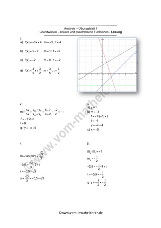
  • 1. ©www.vom-mathelehrer.de Analysis – Übungsblatt 1 Grundwissen – lineare und quadratische Funktionen - Lösung 1. 2. 3. 4. 5. a) f(x) = −3x + 4 m = −3 ; t = 4 b) f(x) = x − 2 m =1 ; t = −2 c) f(x) = −2 m = 0 ; t = −2 d) f(x) = 3 5 x + 3 2 m = 3 5 ; t = 3 2 m = Δy Δx = yQ − yP xQ − xP = 5 − 7 4 − 2 = −2 2 = −1 7 = −1⋅ 2+ t t = 9 g: y = −x +9 a) y =1 b) m = −1 1= −1⋅(−5) + t t = −4 y = −x − 4 c) x = −5 m = tan(30°) = 3 3 −0,5 = 3 3 ⋅3+ t t = −0,5 − 3 y = 3 3 x −0,5 − 3 mg ⋅mf = −1 mg = − 1 2 −2,5 = − 1 2 ⋅ 4+ t t = −0,5 = − 1 2 g: y = − 1 2 x − 1 2
  • 2. ©www.vom-mathelehrer.de 6. a) Normalform entspricht hier Scheitelpunktform S(0 | −2) Y(0 | −2) f(x) = x2 − 2 = (x − 2)(x + 2) N1 ( 2 | 0) ; N2 (− 2 | 0) b) f(x) = x2 − 4x +3 = x2 − 4x + 4 −1 = (x − 2)2 −1 S(2 | −1) Y(0 | 3) x1,2 = 4± 16 −12 2 = 4± 2 2 (Alternative : Vieta) x1 =1 ; x2 = 3 N1 (1| 0) ; N2 (3 | 0) c) f(x) = −2x2 − 4x +3 = −2[x2 + 2x −1,5] = −2[x2 + 2x +1− 2,5] = −2[(x +1)2 − 2,5] = −2(x +1)2 +5 S(−1| 5) Y(0 | 3) x1,2 = 4± 16+ 24 −4 = 4± 2 10 −4 N1 − 2+ 10 2 | 0 ⎛ ⎝ ⎜ ⎜ ⎞ ⎠ ⎟ ⎟; N2 −2+ 10 2 | 0 ⎛ ⎝ ⎜ ⎜ ⎞ ⎠ ⎟ ⎟ d) f(x) = x2 + 2x = x(x + 2) = x2 + 2x +1−1= (x +1)1 −1 S(−1| −1) Y(0 | 0) N1 (0 | 0) ; N2 (−2 | 0) Alternative : x −Koordinate von S liegt wegen Symmetrie zwischen Nst. S(−1| y) y durch einsetzen bestimmen. " # $ $ $ % & ' ' '
  • 3. ©www.vom-mathelehrer.de 7. 8. Wenn man die gegebenen Punkte in die Gleichung y = ax2 + bx + c einsetzt, ergibt sich das Gleichungssystem: Daraus ergibt sich a = -1, b = -6 und c = -7, also y = - x2 - 6x - 7. Scheitelpunktform: y = - (x+3)2 + 2 , also S(-3/2). Nullstellen: e) f(x) = 2(x −3)(x + 2) N1 (−2 | 0) ; N2 (3 | 0) Y(0 | −12) S(0,5 | y); f(0,5) = −12,5 f(x) = 2(x −0,5)2 −12,5 f(x) = a(x − d)2 + e f(x) = a(x +0,5)2 −0,5 = a⋅0,52 a = −2 f(x) = −2(x +0,5)2 I. − 1 4 = 81 4 a − 9 2 b + c II. 1= 4a − 2b+ c III. − 2= a − b+ c x1 =−3 − 2 und x2 = −3+ 2.
  • 4. ©www.vom-mathelehrer.de Analysis – Übungsblatt 2 Grundwissen - ganzrationale Funktionen - Lösung 1. a) f(x) = x(x+2)2 eine einfache NSt bei 0 mit VzW und eine doppelte bei – 2 ohne VzW b) f(x) = x(x2 + 2x + 3) eine einfache NSt bei 0 mit VzW c) f(x) = (x + 1)(x3 + 9x2 + 26x + 24) = (x + 1)(x + 2)(x2 + 7x + 12) = = (x + 1)(x + 2)(x + 3)(x + 4) vier einfache NSt bei -1, -2, -3 und -4 mit VzW 2. . Da die höchste Potenz einen geraden Exponenten besitzt und einen negativen Koeffizienten verläuft der zugehörige Graph von „links unten“ nach „rechts unten“. . Da die höchste Potenz einen ungeraden Exponenten besitzt und den positiven Koeffizienten +1, verläuft der zugehörige Graph von „links unten“ nach „rechts oben“. 3. 4. 5. A(1|0) , B(3|0) , C(-1|0) f(x) = (x2 −3x)(x − x2 ) = x3 − x4 −3x2 +3x3 = −x4 + 4x3 −3x2 4 x- h(x) = −34 + x3 −5x2 = x3 −5x2 −81 x3 f(x) = a x − x1( ) x − x2( ) x − x3( ) und f(0) = 2 f(x) = (x −1)(x +1)(x − 2) = x3 − 2x2 − x + 2 (x4 − 5x3 − 30x2 + 40x + 64) :(x +1) = x3 − 6x2 − 24x + 64 −(x4 + x3 ) − 6x3 − 30x2 −(−6x3 − 6x2 ) − 24x2 + 40x −(−24x2 − 24x) 64x + 64 −(−64x + 64) 0
  • 5. ©www.vom-mathelehrer.de 6. a) -> Der Graph von f ist punktsymmetrisch bezüglich des Koordinatenursprungs. b) => Da für den Graphen von f weder noch gilt, liegt keine Achsensymmetrie bezüglich der y-Achse und auch keine Punktsymmetrie bezüglich des Koordinatenursprungs vor. 7. a) bedeutet, dass der Graph von f an der y-Achse gespiegelt wird. Der Faktor 2 bewirkt, dass zusätzlich noch eine Streckung in y-Richtung (von der x-Achse aus) um den Faktor 2. b) bewirkt, dass der Graph von f in x-Richtung (von der y-Achse aus) mit dem Faktor 2 gestreckt wird. Der Summand +2 bedeutet, dass der Graph zusätzlich um 2 Einheiten nach oben verschoben wird. 8. a) b) c) d) e) f(−x) = 3(−x)3 (2−(−x)2 ) = −3x3 (2− x2 ) = −f(x) f(−x) = (−x + 2)2 (−x)3 = −(2− x)2 x3 f(−x) = f(x) f(−x) = −f(x) f(−x) f( 1 2 x) lim x→+∞ 5 − 1 x2 →+∞ ! →0 ! ⎛ ⎝ ⎜ ⎜ ⎜ ⎜ ⎜ ⎞ ⎠ ⎟ ⎟ ⎟ ⎟ ⎟ = 5 ; lim x→+∞ 5 − 1 x2 →+∞ ! →0 ! ⎛ ⎝ ⎜ ⎜ ⎜ ⎜ ⎜ ⎞ ⎠ ⎟ ⎟ ⎟ ⎟ ⎟ = 5 lim x→+∞ 2−x = 0 ; lim x→−∞ 2−x = +∞ lim x→+∞ (2x3 + x − 3) = +∞ ; lim x→−∞ (2x3 + x − 3) = −∞ lim x→+∞ (2x3 − x − 3) = +∞ ; lim x→−∞ (2x3 − x − 3) = +∞ lim x→+∞ (x − 2x3 −3) = lim x→+∞ (−2x3 + x −3) = −∞ lim x→−∞ (x − 2x3 −3) = lim x→−∞ (−2x3 + x −3) = +∞
  • 6. ©www.vom-mathelehrer.de Analysis – Übungsblatt 3 Gebrochenrationale Funktionen 1- Lösung 1. a) b) c) d) e) f) Definitionsmenge : x − 2 = 0 ↔ x = 2 → D = IR {2} Nullstelle : 5x + 4 = 0 ↔ x = − 4 5 Definitionsmenge : x + 4 = 0 ↔ x = −4 → D = IR {−4} Nullstellen: 2x2 +1= 0 ↔ x2 = − 1 2 → keine Nst., da keine Zahl mit sich selbst multipliziert − 1 2 ergibt. Definitionsmenge : x2 − 4 = 0 ↔ x2 = 4 ↔ x = ±2 → D = IR {−2; 2} Nullstellen: −2x2 − 3x + 9 = 0 x1,2 = 3± 9+ 72 −6 = 3± 9 −6 ; x1 = −2 (keine Nst, da nicht in Definitionsmenge enthalten) x2 =1 f(x) = x2 − 4 x + 2 = (x + 2)(x − 2) x + 2 = x − 2 Definitionsmenge : x + 2 = 0 ↔ x = −2 → D = IR {−2} Nullstellen: x2 − 4 = 0 ↔(x + 2)(x − 2) = 0 x1 = −2 (keine Nst., da nicht in der Definitionsmenge enthalten) x2 = 2 f(x) = 3x2 − 3 x −1 = 3(x2 −1) x −1 = 3(x −1)(x +1) x −1 = 3(x +1) Definitionsmenge : D = IR {1} Nullstelle : x = −1 f(x) = 6x2 − 4x − 42 x −3 Definitionsmenge : D = IR {3} Nullstellen: x1,2 = 4± 16+1008 12 = 4±32 12 x1 = 3 (keine Nst.) x2 = − 7 3 → f(x) = 6x +14 (Definitionsmenge bleibt erhalten; Polynomdivision)
  • 7. ©www.vom-mathelehrer.de 2. 3. f(x) = 1 x − 2 +3 = 1 x − 2 + 3(x − 2) x − 2 = 1+3x − 6 x − 2 = 3x −5 x − 2 f(x) = 1 x +1 − 1 x +3 = x +3 (x +1)(x +3) − x +1 (x +1)(x +3) = (x +3) −(x +1) (x +1)(x +3) = 2 (x +1)(x +3) (1. Term) = 2 x2 +3x + x +3 = 2 x2 + 4x +3 (2. Term) = 2 x2 + 4x + 4 −1 = 2 (x + 2)2 −1 = 1 1 2 [(x + 2)2 −1] = 1 0,5(x + 2)2 −0,5 (3. Term) Evtl. einf acher : 3. Term ausmultiplizieren und zu 2. Term umformen!!!
  • 8. ©www.vom-mathelehrer.de Analysis – Übungsblatt 4 Gebrochenrationale Funktionen 2 - Lösung 1. a) b) c) d) e) f) f(x) = 5x + 4 x − 2 ; D = IR {2} lim x→2 > 5x + 4 →14!"# x − 2 +0 ! ⎛ ⎝ ⎜ ⎜ ⎜ ⎜ ⎞ ⎠ ⎟ ⎟ ⎟ ⎟ = +∞ ; lim x→2 < 5x + 4 →14!"# x − 2 −0 ! ⎛ ⎝ ⎜ ⎜ ⎜ ⎜ ⎞ ⎠ ⎟ ⎟ ⎟ ⎟ = −∞ ; Polstelle mit VZW f(x) = 2x2 +1 x + 4 ; D = IR {−4} lim x→−4 > 2x2 +1 33!"# x + 4 +0 ! ⎛ ⎝ ⎜ ⎜ ⎜ ⎜ ⎞ ⎠ ⎟ ⎟ ⎟ ⎟ = +∞ ; lim x→−4 < 2x2 +1 33!"# x + 4 −0 ! ⎛ ⎝ ⎜ ⎜ ⎜ ⎜ ⎞ ⎠ ⎟ ⎟ ⎟ ⎟ = −∞ ; Polstelle mit VZW f(x) = −2x2 −3x +9 x2 − 4 ; D = IR {−2;2} lim x→−2 > −2x2 −3x +9 →7! "## $## x2 − 4 →−0 %&' ⎛ ⎝ ⎜ ⎜ ⎜ ⎜ ⎞ ⎠ ⎟ ⎟ ⎟ ⎟ = −∞ ; lim x→−2 < −2x2 −3x +9 →7! "## $## x2 − 4 →−0 %&' ⎛ ⎝ ⎜ ⎜ ⎜ ⎜ ⎞ ⎠ ⎟ ⎟ ⎟ ⎟ = +∞ ; Polstelle mit VZW lim x→2 > −2x2 −3x +9 →−5! "## $## x2 − 4 →+0 %&' ⎛ ⎝ ⎜ ⎜ ⎜ ⎜ ⎞ ⎠ ⎟ ⎟ ⎟ ⎟ = −∞ ; lim x→−2 < −2x2 −3x +9 →−5! "## $## x2 − 4 →−0 %&' ⎛ ⎝ ⎜ ⎜ ⎜ ⎜ ⎞ ⎠ ⎟ ⎟ ⎟ ⎟ = +∞ ; Polstelle mit VZW f(x) = x2 − 4 x + 2 = (x + 2)(x − 2) x + 2 = x − 2 ; D = IR {−2} lim x→2 > x − 2( )= 0 ; lim x→2 < x − 2( )= 0 ; hebbare Definitionslücke f(x) = 3x2 −3 x −1 = 3(x2 −1) x −1 = 3(x −1)(x +1) x −1 = 3(x +1) ; D = IR {1} lim x→1 > 3(x +1)( )= 6 ; lim x→1 < 3(x +1)( )= 6 ; hebbare Definitionslücke f(x) = 6x2 − 4x − 42 x −3 = 6x +14 ; D = IR {3} lim x→3 > 6x +14( )= 32 ; lim x→−3 < 6x +14( )= 32 ; hebbare Definitionslücke
  • 9. www.vom-mathelehrer.de Analysis – Übungsblatt 5 Gebrochen-rationale Funktionen 3 - Lösung 1. a) b) c) f(x) = 5x + 4 x − 2 ; D = IR {2} lim x→±∞ 5x + 4 x − 2 ⎛ ⎝ ⎜ ⎞ ⎠ ⎟ = 5 ("z = n" → Vergleiche Leitkoeffizienten) Alternative : lim x→±∞ 5x + 4 x − 2 ⎛ ⎝ ⎜ ⎞ ⎠ ⎟ = lim x→±∞ x 5+ 4 x ⎛ ⎝ ⎜ ⎞ ⎠ ⎟ x 1− 2 x ⎛ ⎝ ⎜ ⎞ ⎠ ⎟ ⎛ ⎝ ⎜ ⎜ ⎜ ⎜ ⎞ ⎠ ⎟ ⎟ ⎟ ⎟ = lim x→±∞ 5+ 4 x →±0! 1− 2 x →±0 " ⎛ ⎝ ⎜ ⎜ ⎜ ⎜ ⎜ ⎜ ⎞ ⎠ ⎟ ⎟ ⎟ ⎟ ⎟ ⎟ = 5 Sprichen Sie mit Ihrem Mathelehrer, was er sehen möchte! senkr : x = 2 waagr : y = 5 f(x) = 2x2 +1 x + 4 = 2x −8+ 33 x + 4 ; D = IR {−4} lim x→−∞ 2x −8+ 33 x + 4 →0 ! ⎛ ⎝ ⎜ ⎜ ⎜ ⎞ ⎠ ⎟ ⎟ ⎟ = −∞ ; lim x→+∞ 2x −8+ 33 x + 4 →0 ! ⎛ ⎝ ⎜ ⎜ ⎜ ⎞ ⎠ ⎟ ⎟ ⎟ = +∞ senkr.: x = −4 schräg: y = 2x −8 ("z = n+1") f(x) = −2x2 −3x +9 x2 − 4 ; D = IR {−2;2} lim x→−∞ −2x2 −3x +9 x2 − 4 ⎛ ⎝ ⎜⎜ ⎞ ⎠ ⎟⎟ = −2 ; lim x→+∞ −2x2 −3x +9 x2 − 4 ⎛ ⎝ ⎜⎜ ⎞ ⎠ ⎟⎟ = −2 ("z = n" → Vergleiche Leitkoeffizienten) senkr : x = −2 ; x = 2 waagr : y = −2
  • 10. www.vom-mathelehrer.de d) e) f) 2. f(x) = x2 − 4 x + 2 = (x + 2)(x − 2) x + 2 = x − 2 ; D = IR {−2} lim x→−∞ > x − 2( )= −∞ ; lim x→+∞ x − 2( )= +∞ f(x) = 3x2 −3 x −1 = 3(x2 −1) x −1 = 3(x −1)(x +1) x −1 = 3(x +1) ; D = IR {1} lim x→−∞ 3(x +1)( )= −∞ ; lim x→+∞ 3(x +1)( )= +∞ f(x) = 6x2 − 4x − 42 x −3 = 6x +14 ; D = IR {3} lim x→−∞ 6x +14( )= −∞ ; lim x→+∞ 6x +14( )= +∞ f(x) = 20x x2 − 25 = 20x (x −5)(x +5) Betrachte die Nennernullstellen für die Definitionsmenge! → D = IR {−5; 5} Symmetrie : f(−x) = 20(−x) (−x)2 − 25 = −20x x2 − 25 = − 20x x2 − 25 = f(x) → Punktsymmetrie bzgl. (0 | 0) senkr.: x = −5 ; x = 5 waagr.: y = 0 ("z < n")
  • 11. www.vom-mathelehrer.de 3. I: Steigung passt nicht II: passt nicht, das Polstelle mit VZW im Graph dargestellt ist, die Funktionsgleichung jedoch eine Nullstelle ersten Grades besitzt. 4. 0 = 1 2 ⋅(−1) −1+ a (−1−1)2 0 = −1,5+ a 4 a = 6 a) D = IR {1} SX (−3 | 0) SY (0 | −9) b)x + 7+ 16 x −1 = x(x −1) x −1 + 7(x −1) x −1 + 16 x −1 = x2 − x + 7x − 7+16 x −1 = x2 + 6x +9 x −1 = (x +3)2 x −1 = f(x) oder bei f(x) Zähler ausmultiplizieren und Polynomdivision durchführen. g ist schräge Asymptote von Gf .
  • 12. www.vom-mathelehrer.de Analysis – Übungsblatt 6 Differenzenquotient – mittlere Änderungsrate Differentialquotient – lokale Änderungsrate - Lösung 1. 2a) b) 3. 4a) A(0 | 730) ; B(21000 | 2962) Durchschn. Steigung: m = Δy Δx = yB − yA xB − xA = 2969 − 730 21000 −0 = 2239 21000 ≈ 0,107 Steigungswinkel: m = tan(α) = Gegenkathete Ankathete = Δy Δx = yB − yA xB − xA α = tan−1 2239 21000 ⎛ ⎝ ⎜ ⎞ ⎠ ⎟ ≈ 6,09° I1 : f(b) − f(a) b − a = 5⋅52 −5⋅ 22 5 − 2 = 355 3 I2 : f(b) − f(a) b − a = 5⋅ 42 −5⋅ 22 4 − 2 = 30 I3 : f(b) − f(a) b − a = 5⋅32 −5⋅ 22 3 − 2 = 25 f '(x0 ) = lim x→x0 f(x) − f(x0 ) x − x0 = lim x→2 f(x) − f(2) x − 2 = lim x→2 5x2 − 5⋅ 22 x − 2 = lim x→2 5(x2 − 4) x − 2 = lim x→2 5(x + 2)(x − 2) x − 2 = = lim x→2 5(x + 2) = 5⋅(2+ 2) = 20 = f '(2) f '(x0 ) = lim x→x0 f(x) − f(x0 ) x − x0 = lim x→−1 f(x) − f(−1) x −(−1) = lim x→2 1 5 x2 − 1 2 x + 2−( 1 5 ⋅(−1)2 − 1 2 ⋅(−1) + 2) x +1 = = lim x→−1 1 5 x2 − 1 2 x + 2− 1 5 − 1 2 − 2 x +1 = lim x→−1 1 5 x2 − 1 2 x − 7 10 x +1 = lim x→−1 x − 7 2 ⎛ ⎝ ⎜ ⎞ ⎠ ⎟ x +1( ) x +1 = lim x→−1 x − 7 2 ⎛ ⎝ ⎜ ⎞ ⎠ ⎟ = − 9 2 NR : x1,2 = 1 2 ± 1 4 + 4⋅ 1 5 ⋅ 7 10 2 5 = 1 2 ± 81 100 2 5 x1 = 7 2 ; x2 = −1 ⎛ ⎝ ⎜ ⎜ ⎜ ⎜ ⎜ ⎜ ⎜ ⎞ ⎠ ⎟ ⎟ ⎟ ⎟ ⎟ ⎟ ⎟ n(t) = 3t2 − 60t + 500 m = n(2) −n(0) 2− 0 = 3⋅ 22 − 60⋅ 2+ 500 − 500 2 = −54 mittlere Änderungsrate : −54 1 h I": f(b) − f(a) b − a = 5 ∙ 5- − 5 ∙ 2- 5 − 2 = 35
  • 13. www.vom-mathelehrer.de 5) f(x) = 2x ⋅e−0,5x2 mS = f(0,5) − f(−0,5) 0,5 −(−0,5) = e−0,53 −(−e−0,53 ) 1 = 2e−0,53 ≈ 1,76 f '(x) = 2⋅e−0,5x2 + 2x ⋅e−0,5x2 ⋅(−x) = 2e−0,5x2 (1− x2 ) mT = f '(0) = 2e0 (1−0) = 2 mT −mS mT ≈ 0,12 =12%
  • 14. www.vom-mathelehrer.de Analysis – Übungsblatt 7 Tangente –- Ableitung – Stammfunktion - Lösung 1) 2) 3) 4) g f(x) = 5x2 f '(x) =10x m = f '(2) = 20 y = mx + t 20 = 20⋅ 2+ t ↔ t = −20 y = 20x − 20 f(x) = 1 5 x2 − 1 2 x + 2 f '(x) = 2 5 x − 1 2 m = f '(−1) = − 9 10 y = mx + t 27 10 = − 9 10 ⋅(−1) + t ↔ t =1,8 y = − 9 10 x +1,8 F(x) = x2 − 2x F'(x0 ) = lim x→x0 x2 − 2x − x0 2 − 2x0( ) x − x0 = lim x→x0 x2 − x0 2 −(2x − 2x0 ) x − x0 = lim x→x0 (x − x0 )(x + x0 ) x − x0 − lim x→x0 2(x − x0 ) x − x0 = lim x→x0 x + x0( )− 2 = 2x0 − 2 = f(x0 ) Definitionsmengen vergleichen!!! → F ist Stammfunktion zu f
  • 15. www.vom-mathelehrer.de 5) lim t→t0 3t2 − 60t +500 −(3t0 2 − 60t0 +500) t − t0 = lim t→t0 3t2 − 60t −3t0 2 + 60t0 t − t0 = lim t→t0 3t2 −3t0 2 −(60t − 60t0 ) t − t0 = lim t→t0 3t2 −3t0 2 0 t − t0 − lim t→t0 60t − 60t0 t − t0 = lim t→t0 3(t − t0 )(t + t0 ) t − t0 − lim t→t0 60(t − t0 ) t − t0 = lim t→t0 3(t − t0 ) − 60 = 6t0 − 60 f '(x) = 6t − 60 (Später ohne Diff '− qu ableiten!!!) −30 = 6t − 60 6t = 30 t = 5 5 Stunden nach Beginn...
  • 16. www.vom-mathelehrer.de Analysis – Übungsblatt 8 Summen- und Faktorregel - Lösung 1) 2) 3) An diesen Stellen besitzt der Graph eine Tangente, die parallel zur x-Achse verläuft. 4) 5) f(x) = x3 − x2 + x +1 ; f '(x) = 3x2 − 2x +1 g(x) = 1 3 x3 − 1 2 x2 + x +1 ; g'(x) = x2 − x +1 h(x) =18 − x3 + 3x2 ; h'(x) = −3x2 + 6x i(x) = −3 ; i'(x) = 0 j(x) = 4x(x −1)2 = 4x(x2 − 2x +1) = 4x3 − 8x2 + 4x ; j'(x) =12x2 −16x + 4 k(x) = 1 x −1= x−1 −1 ; k'(x) = −x−2 = − 1 x2 l(x) = 5 x2 + 5x 2 = 5x−2 + 5 2 x ; l'(x) = −10x−3 + 2,5 = − 10 x3 + 2,5 f(x) = x3 − 2x2 ; f '(x) = 3x2 − 4x f(2) = 0 f '(2) = 4 y = mx + t 0 = 4⋅ 2+ t ↔ t = −8 y = 4x −8 f(x) = x3 − 6x2 +11x − 6 f '(x) = 3x2 −12x +11 f ''(x) = 6x −12
  • 17. www.vom-mathelehrer.de Analysis – Übungsblatt 9 Produkt- und Quotientenregel - Lösung 1) 2a) Definitionslücken: egal Nullstellen: I Asymptoten: III SP y-Achse: II b) 3a) b) Ist die Kettenregel bekannt, kann diese Aufgabe „geschickter“ gelöst werden. 4) f '(x) =1⋅(x2 + x +1) +(x −1)(2x +1) = x2 + x +1+ 2x2 + x − 2x −1= 3x2 g'(x) = (x − 2)⋅1− x ⋅1 (x − 2)2 = −2 (x − 2)2 h'(x) = (2x −3)⋅(2x −1) −(x2 − x)⋅ 2 (2x −3)2 = 2x2 − 6x +3 (2x −3)2 i'(x) = 0 j(x) = 4x(x −1)2 = 4x(x2 − 2x +1) = 4x3 − 8x2 + 4x ; j'(x) =12x2 −16x + 4 k(x) = 1 x −1= x−1 −1 ; k'(x) = −x−2 = − 1 x2 l(x) = 5 x2 + 5x 2 = 5x−2 + 5 2 x ; l'(x) = −10x−3 + 2,5 = − 10 x3 + 2,5 f '(x) = x2 + 4x +13 (x + 2)2 I: 4x = 0 ↔ x = 0 II: senkr : x = −1 III: "z < n" f(x) = 4x (x +1)2 = 4x x2 + 2x +1 f '(x) = (x2 + 2x +1)⋅ 4 − 4x ⋅(2x + 2) (x +1)4 = 4(x +1)2 −8x(x +1) (x +1)4 = (x +1)[4(x +1) −8x] (x +1)4 = 4x + 4 −8x (x +1)3 = −4x + 4 (x +1)3 D = IR {− 5 4 } f '(x) = (4x +5)⋅ 2−(2x +3)⋅ 4 (4x +5)2 = 4x +10 −8x −12 (4x +5)2 = − 2 (4x +5)2
  • 18. www.vom-mathelehrer.de Analysis – Übungsblatt 10 Monotonie und Extrempunkte - Lösung 1) f '(x) = 3x2 − x +1 f '(x)= ! 0 3x2 − x +1= 0 x1,2 = 1± 1−12 6 ; keine Nullstelle der ersten Ableitung → keine waagrechte Tangete an Gf → kein Extremum Monotonie : f '(x) > 0 für alle x ∈ ID f ist streng monoton wachsend. g'(x) = (x − 2)⋅1− x ⋅1 (x − 2)2 = −2 (x − 2)2 ; Dg = Dg' = IR {2} g'(x) ≠ 0 ; keine Nullstellen der ersten Ableitung → keine waagrechte Tangete an Gf → kein Extremum Monotonie : x : − − − − − + 2 Def.−L − − − −− > f '(x) : < 0 < 0 Gf fällt fällt
  • 19. www.vom-mathelehrer.de h'(x) = (2x −3)⋅(2x −1) −(x2 − x)⋅ 2 (2x −3)2 = 2x2 − 6x +3 (2x −3)2 ; Dh = Dh' = IR {1,5} h'(x)= ! 0 2x2 − 6x +3 = 0 x1,2 = 6± 36 − 24 4 = 6± 2 3 4 x1 = 3+ 3 2 ; x2 = 3 − 3 2 Gf besitzt waagrechte Tangente; potentielle Extrempunkte( ) Monotonie : x : − − − − − + 3− 3 2 − − − − − − + 1,5 Def.−L − − − − − − + 3+ 3 2 − − − − − − > f '(x) : > 0 < 0 < 0 > 0 Gf : steigt fällt fällt steigt HOP TIP 3 − 3 2 | 2− 3 2 ⎛ ⎝ ⎜ ⎜ ⎞ ⎠ ⎟ ⎟ 3+ 3 2 | 2+ 3 2 ⎛ ⎝ ⎜ ⎜ ⎞ ⎠ ⎟ ⎟ l'(x) = −10x−3 + 2,5 = − 10 x3 + 2,5 ; Dl = Dl' = IR {0} l'(x)= ! 0 − 10 x3 + 2,5 = 0 ↔ 10 x3 = 2,5 ↔ x3 = 4 ↔ x = 43 Monotonie : x : − − − − − − + 0 Def.−L − − − − − − + 43 − − − − − − > f '(x) : > 0 < 0 > 0 Gf : steigt fällt steigt TIP 43 | 5,95( )
  • 20. www.vom-mathelehrer.de 2a) b) 3) z.B. lim x→+∞ 1 a >0 x →+∞ ( x2 →+∞ −1) ⎛ ⎝ ⎜ ⎜ ⎞ ⎠ ⎟ ⎟ = +∞ → Abbildung 2 fa '(x) = 3 a ⋅ x2 −1 fa '(x)= ! 0 3 a ⋅ x2 −1= 0 ↔ x2 = a 3 ↔ x1,2 = ± a 3 x −Koord. des Extrempunkts einsetzen: 3 = ± a 3 9 = a 3 ↔ a = 27 → f27 (x) = 1 27 x3 − x ; f '27 (x) = 1 9 x2 −1 Pr obe auf Extrempunkt : (da Gf punktsymm. bzgl. (0 | 0) ist, wird Monotonie für x > 0 untersucht) x : − − − − −+ 3 − − − −− > f '(x) : < 0 > 0 Gf fällt steigt TIP Ist die zweite Ableitung bekannt : f ''a (x) = 6 a x ; f ''27 (3) = 6 27 ⋅3 ≠ 0 ⎛ ⎝ ⎜ ⎜⎜ ⎞ ⎠ ⎟ ⎟⎟ f '(x) = 4x3 − 6x2 f '(x)= ! 0 4x3 − 6x2 = 0 2x2 (2x −3) = 0 x1 = 0 ; x2 =1,5 Monotonie : x : − − − − − −+ 0 − − − − − − + 1,5 − − − −− > f '(x) : < 0 < 0 > 0 Gf : fällt fällt steigt TEP TIP aus a) bekannt 1,5 | −1,69( )
  • 21. www.vom-mathelehrer.de Analysis–Übungsblatt11 Kurvendiskussion -LösungKurvendiskussionrationalerFunktionen UmbestimmteEigenschaftendesGraphenablesenzukönnen,eignensichunterschiedlicheDarstellungsformendesFunktionsterms: 1.Definitionsmenge DieDefinitionsmengeistentwederangegeben(z.B.beiAnwendungsbezügen),ansonsten istdiemaximaleDefinitionsmengefür -ganz-rationaleFunktionenganzIR. -gebrochen-rationaleFunktionenganzIRohnegegebenenfallsdie Nennernullstellen. 2.Symmetrie AllgemeinerAnsatzzurUntersuchung: -f(–x)=f(x) ÞAchsensymmetriezury-Achse -f(–x)=–f(x) ÞPunktsymmetriezumUrsprung Speziellfürganz-rationaleFunktionen: -nurgeradeExponenten ÞAchsensymmetrie -nurungeradeExponenten ÞPunktsymmetrie HatdieFunktioneineSymmetrie,kannmansichoftdieHälftederArbeit„sparen“! f(x)= x3 x2 −1 = x3 (x+1)(x−1) =x+ x x2 −1 Df =IR{−1;1} f(−x)= (−x)3 (−x)2 −1 = (−1)3 x3 (−1)2 x2 −1 =− x3 x2 −1 =−f(x) →PunktsymmetriezumKoordinatenursprung.
  • 22. www.vom-mathelehrer.de 3.SchnittpunktmitdenKoordinatenachsen Schnittpunktmitdery-AchseSy(0/f(0)):f(0)=yo Schnittpunktmitderx-AchseSx(x0/0):f(x)=0 StrategienbeiderNullstellensuche: -Ausklammern,wennmöglich,vonxn Þn-facheNullstellebeixo=0 -ErrateneinerNullstellex1ÞPolynomdivisiondesFunktionstermsdurch(x–x1) -QuadratischeTermemitLösungsformelauswerten -LineareGleichungenmitÄquivalenzumformungauflösen DieVielfachheiteinerNullstelleermöglichteinigeinteressanteSchlussfolgerungen: -UngeradeVielfachheitÞVorzeichenwechsel(geradeVielfachheitÞkeinVZW) -DieVielfachheiteinerNullstelleistinderAbleitungumeinsniedriger! -DieVielfachheitverrätetwasüberdenVerlaufdesGrapheninderUmgebungder Nullstelle: oEinfacheNullstelle:SchnittpunktwiebeieinerGeradenmitderx-Achse oDoppelteNullstelle:Berührpunkt(wiebeiParabel),lokalerExtrempunkt oDreifacheNullstelle:TerrassenpunktanderNullstelle f(0)= 03 02 −1 =0 →Sy (0/0) f(x)=0 x3 x2 −1 =0⇔x3 =0⇔x=0 dreifacheNullstelle  →Sx (0/0)
  • 23. www.vom-mathelehrer.de 4.VerhaltenimUnendlichen Beiganz-rationalenFunktionenbestimmtderSummandmitdemgrößtenExponentendas Verhaltenfürf(x). Fürgebrochen-rationaleFunktionengiltfürdenZählergradzunddenNennergradn -z<n:x-AchseistwaagrechteAsymptote -z=n:waagrechteAsymptote -z=n+1:schrägeAsymptote -z>n+1:keineAsymptote ZurBestimmungderAsymptoteneignensich: •SenkrechteAsymptoten:Nennernullstellen,sofernsiesichnichtgegen Zählernullstellenkürzenlassen •WaagrechteAsymptoten:AusklammernundKürzenderhöchstenvorkommenden Potenz,fallsz<noderz=n •SchrägeAsymptoten:DurchführungderPolynomdivision,fallsz>n 5.VerhaltenandenDefinitionslücken (fürgerochen-rationaleFunktionen) WirdderNenner,jedochnichtderZähler,fürxpnull,sobesitztdieFunktionhiereine Polstelle.DerGraphbesitzteinesenkrechteAsymptotemitderGleichungx=xp. HabenZählerundNennergemeinsameNullstellen,sozerlegtmanbeideinLinearfaktoren undkürzt.DamitkannmanDefinitionslückenbeheben. lim x→−∞ x+ x x2 −1 =lim x→−∞ x+ x2 ⋅ 1 x x2 (1− 1 x2 ) =lim x→−∞ x →−∞ + 1 x →0 1− 1 x2 →0  →0  =−∞ lim x→+∞ x+ x x2 −1 =lim x→+∞ x+ x2 ⋅ 1 x x2 (1− 1 x2 ) =lim x→+∞ x →+∞ + 1 x →0 1− 1 x2 →0  →0  =+∞ lim x→xp f(x)=±∞ lim x→ < −1 x3 →−1 x2 −1 →+0  =−∞lim x→ < 1 x3 →1 x2 −1 →−0  =−∞ lim x→ > −1 x3 →−1 x2 −1 →−0  =+∞lim x→ > 1 x3 →1 x2 −1 →+0  =+∞
  • 26. www.vom-mathelehrer.de Analysis – Übungsblatt 12 Newton und Umkehrfunktion - Lösung 1) Die Tangenten an den Graphen in Hoch- bzw. Tiefpunkt sind parallel zur x-Achse. Dadurch existiert kein Schnittpunkt von Tangente und x-Achse und das Verfahren kann nicht ausgeführt werden. ODER: 2) 3) 4) xn+1 = xn − f(xn ) f '(xn ) Im Extermpunkt gilt f '(xn ) = 0 → Durch Null darf nicht dividiert werden. → Verfahren kann nicht ausgeführt werden. f−1 x( )= 1 x Df−1 = IR {0} Wf−1 = IR {0} f x( )=1+ 1 x y =1+ 1 x ↔ y −1= 1 x ↔ x = 1 y −1 f−1 (x) = 1 x −1 Df−1 = IR {1} Wf−1 = IR {0} y = 2x 1+5x ↔(1+5x)y = 2x ↔ y +5xy = 2x ↔ y = 2x −5xy ↔ y = x(2−5y) ↔ x = y 2−5y f−1 x( )= x 2−5x Df−1 = IR { 2 5 } Wf−1 = IR {− 1 5 }
  • 27. www.vom-mathelehrer.de 5) Gf ist achsensymmetrisch bzgl. der Winkelhalbierenden des 1. Und 3. Quadranten. 6) Nicht umkehrbar auf IR, da jede Parallele zur x-Achse mit der Gleichung y=a mit -1≤a≤1 Gf unendlich oft schneidet. Mögliches Intervall I=[0; π]
  • 28. www.vom-mathelehrer.de Analysis – Übungsblatt 13 Trigonometrische Funktionen - Lösung 1) 2) z.B.: a=6 3 α) z.B.: a=1; c=1 β) z.B.: a=2; c=0 4) a)k=π b) f(x) = sin(x) + cos(x) ; f '(x) = cos(x) − sin(x) g(x) = 1 2 cos(x) − 1 2 sin(x) ; g'(x) = − 1 2 sin(x) − 1 2 cos(x) h(x) = 3 ⋅cos(x) ; h'(x) = − 3 ⋅sin(x) i(x) = − 3 ⋅cos(x) ; i'(x) = 3 ⋅sin(x) j(x) = x + 3 ⋅sin(x) ; j'(x) =1+ 3 ⋅cos(x) k(x) = 1 9 x3 ⋅cos(x) ; k'(x) = 1 3 x2 ⋅cos(x) − 1 9 x3 ⋅sin(x) (Produktregel) y = x +k mit k ≠ 0 z.B.: y = x −1
  • 29. www.vom-mathelehrer.de Analysis – Übungsblatt 14 Funktionen mit rationalen Exponenten - Lösung 1) 2a) b) 3) f(x) = x = x 1 2 ; Df = IR+ 0 ; f '(x) = 1 2 x − 1 2 = 1 2 x g(x) = 1 x = x − 1 2 ; Dg = IR+ ; g'(x) = − 1 2 x − 3 2 = − 1 2x x = − x 2x2 h(x) = 3 ⋅ x ; Dh = IR ; h'(x) = 3 i(x) = x x = x x x = x ; Di = IR+ ; i'(x) = 1 2 x j(x) = x + x ; Dj = IR+ 0 ; j'(x) =1+ 1 2 x k(x) = x ⋅cos(x) ; Dk = IR+ 0 ; k'(x) = 1 2 x ⋅cos(x) − x ⋅sin(x) Definitionsmenge : 4+ x ≥ 0 x ≥ −4 Dg = [−4; +∞[ SP mit y − Achse : g(0) = 2⋅ 4+ 0 −1= 3 Sy (0 | 3) Von innen nach außen: x → x + 4 : Verschiebung um 4 Einheiten nach links x + 4 → 2⋅ x + 4 : Streckung um Faktor 2 in y −Richtung 2⋅ x + 4 → 2⋅ x + 4 −1: Verschiebung um 1 Einheit nach unten Wertemenge : Wg = [−1 ; +∞[
  • 30. www.vom-mathelehrer.de x2 −b ≥ 0 x2 ≥ b | x |≥ b x ≥ b oder −x ≥ b ↔ x ≤ − b Dg = IR]− b ; b[ b = 2 → b = 4
  • 31. www.vom-mathelehrer.de Analysis – Übungsblatt 15 Kettenregel - Lösung 1) 2a) f '(x) = 2(3x − 4)3 = 6(3x − 4) h(x) = 3x = (3x) 1 2 ; h'(x) = 1 2 (3x) − 1 2 ⋅3 = 3 2 3x h'(x) = (2x +1) 1 2 = 1 2 ⋅(2x +1) − 1 2 ⋅ 2 = 1 2x +1 i'(x) = cos(x3 −5x)⋅(3x2 −5) j'(x) = 2x3 −19x2 +12x 2(2x +3)4 1− x k(x) = 5x5 ( ) 1 3 ; k'(x) = 1 3 5x5 ( ) − 2 3 ⋅ 25x4 = 25x4 3 5x5 ( ) 2 3 = 25x4 3 25x103 = 25x4 3 25⋅ x9 ⋅ x3 = 25x4 3⋅ 25 1 3 ⋅ x3 ⋅ x3 = 25x ⋅ 25 2 3 3⋅ 25⋅ x3 = x ⋅ 2523 3 x3 = x 53 ⋅53 3 x3 = 5x ⋅ 53 3 x3 Definitionsmenge : 3x − 5 ≥ 0 3x ≥ 5 x ≥ 5 3 D = [ 5 3 ; +∞[ f(3) = 2 f '(x) = 1 2 (3x −5) − 1 2 ⋅3 = 3 2 3x −5 m = f '(3) = 3 2 3⋅3 −5 = 3 4 y = mx + t 2 = 3 4 ⋅3+ t ↔ t = − 1 4 y = 3 4 x − 1 4
  • 32. www.vom-mathelehrer.de f(x)= ! 0 ↔ sinx = 0 ↔ x = kπ (k ∈ Z {0} Definitionsmenge beachten!) (x = 0; ±π; ±2π; ...) f(−x) = sin(−x) (−x)2 = −sin(x) x2 = − sin(x) x2 = −f(x) → Punktsymm. bzgl (0 | 0) Grenzwert : lim x→+∞ sinx Wertemenge [−1;1] ! x2 →+∞ ! = 0 f '(x) = x2 ⋅cosx − sinx ⋅ 2x x4 = x ⋅cosx − 2⋅sinx x3
  • 33. www.vom-mathelehrer.de Analysis – Übungsblatt 16 e- und ln-Funktion - Lösung 1) Df = IR ; f '(x) = e0,5x+1 ⋅0,5 = 0,5e0,5x+1 Dg = IR ; g'(x) = e− 0,5x2 ⋅(−0,5⋅ 2x) = −xe− 0,5x2 Dh = IR {0} ; h'(x) = xex − ex ⋅1 x2 = (x −1)ex x2 Definitionsbereich: x − 2> ! 0 ↔ x > 2 ; Di =]2; +∞[ i'(x) = 1 x − 2 j(x) = ln(x3 ) = 3lnx ; Dj = IR+ j'(x) = 3 x Alternative : j'(x) = 1 x3 ⋅3x2 = 3 x k(x) = ln x + 4 x ⎛ ⎝ ⎜ ⎞ ⎠ ⎟ = ln(x + 4) −lnx Definitionsmenge : x + 4 x > ! 0 ; x + 4 > 0 für x > −4 x + 4 < 0 für x < −4 Betrachte in Vorzeichentabelle Nenner − und Zählernullstellen: x : − − − − − − + −4 − − − − − −+ 0 − − − − − − > f(x) : x + 4 −! x − ! > 0 x + 4 +! x − ! < 0 x + 4 +! x + ! > 0 Dk =]−∞; −4[∪]0;+∞[ k'(x) = 1 x + 4 − 1 x = x x(x + 4) − x + 4 x(x + 4) = x −(x + 4) x(x + 4) = −4 x(x + 4) Alternative : k'(x) = 1 x + 4 x ⋅ x −(x + 4) x2 = x x + 4 ⋅ −4 x2 = −4 x + 4 (Nachdifferenzieren mit Quotientenregel)
  • 34. www.vom-mathelehrer.de 2a) b) c) 3) Definitionsbereich: IR. Symmetrie: Wegen f(-x)=f(x) liegt Achsensymmetrie zur y-Achse vor. fk (−x) = (−x)2 −ln((−x)2 +k2 ) = x2 −ln(x2 +k2 ) = f(x) → Gfk symmetrisch bzgl. y − Achse fk '(x) = 2x − 1 x2 +k2 ⋅ 2x = 2x(x2 +k2 ) − 2x x2 +k2 = 2x(x2 +k2 −1) x2 +k2 =fD lim x→±∞ e− x2 →+∞! 2 −∞!"# $# = 0 f(x) = e − x2 2 f '(x) = e − x2 2 ⋅ − 2x 2 ⎛ ⎝ ⎜ ⎞ ⎠ ⎟ = −xe − x2 2
  • 35. www.vom-mathelehrer.de Analysis – Übungsblatt 17 e- und ln-Gleichungen - Lösung 1) 2) Keine Nullstellen, denn die e-Funktion wird nie Null. ; e2x = 2 ↔ 2x = ln(2) ↔ x = ln(2) 2 e2x+1 −1= 0 ↔ e2x+1 =1↔ 2x +1= ln(1) ↔ 2x +1= 0 ↔ 2x = −1↔ x = − 1 2 3x e0.5x −1( )= 0 x1 = 0 e0,5x −1= 0 ↔ e0,5x =1↔ x = 0, da e0 =1→ x2 = 0 ln(x − 2) = 0 ↔ x − 2 =1↔ x = 3 2ln(x) +3 = 0 ↔ln(x) = −1,5 ↔ x = e−1,5 2xln(x2 −3) = 0 x1 = 0 x2 −3 =1↔ x2 = 4 ↔ x2,3 = ±2 ln x + 4 x ⎛ ⎝ ⎜ ⎞ ⎠ ⎟ = 0 x + 4 x =1↔ x + 4 = x ↔ 0 = 4 → keine Nst. f '(x) = e − x2 2 ⋅(− 1 2 ⋅ 2x) = −xe − x2 2 f '(x)= ! 0 ↔ x = 0 x : − − − − −+ − − − − − > f '(x) : > 0 < 0 Gf : steigt fällt HOP(0 |1)
  • 36. www.vom-mathelehrer.de 3) x + 2 > 0 ↔ x > −2 2− x > 0 ↔ x < 2 Df =]− 2; 2[ ln(x + 2) −ln(2− x) = 0 ln(x + 2) = ln(2− x) | e * x + 2 = 2− x 2x = 0 x = 0 f '(x) = 1 x + 2 ⋅1− 1 2− x ⋅(−1) = 1 x + 2 + 1 2− x = 2− x (x + 2)(2− x) + 2+ x (x + 2)(2− x) = 4 (x + 2)(2− x) f '(x) ≠ 0 ; sogar > 0 → Gf streng monoton wachsend → keine Nullstellen
  • 37. www.vom-mathelehrer.de Analysis – Übungsblatt 18 Zusammengesetzte Funktionen - Lösung 1) f(x) = 3x + 9 = 3x + 9( ) 1 2 ; f '(x) = 1 2 3x + 9( ) − 1 2 ⋅3 = 3 2 3x + 9 = 3 2⋅ 3 ⋅ x + 3 = 3 2 x + 3 Oder : f(x) = 3x + 9 = 3 ⋅ x + 3 = 3 x + 3( ) 1 2 ; f '(x) = 3 ⋅ 1 2 x + 3( ) − 1 2 ⋅1= 3 2 x + 3 f(x) = 2ex ex + 9 ; f '(x) = (ex + 9)⋅ 2ex − 2ex ⋅ex ex + 9( ) 2 = 2e2x +18ex − 2e2x ex + 9( ) 2 = 18ex ex + 9( ) 2 f(x) = x2 ⋅ex ; f '(x) = 2xex + x2 ex f(x) = x lnx ; f '(x) = lnx − x ⋅ 1 x lnx( ) 2 = lnx −1 lnx( ) 2 f(x) = 1−lnx = (1−lnx) 1 2 ; f '(x) = 1 2 (1−lnx) − 1 2 ⋅ − 1 x ⎛ ⎝ ⎜ ⎞ ⎠ ⎟ = − 1 2x 1−lnx f(x) = lnx x2 ; f '(x) = x2 ⋅ 1 x −lnx ⋅ 2x x4 = x − 2xlnx x4 = 1− 2lnx x3 f(x) = (3+ x)2 x −1 ; f '(x) = x2 − 2x −15 x2 − 2x +1 f(x) = 2 (lnx)2 −1( ) ; f '(x) = 2 2lnx( )⋅ 1 x = 4lnx x Alternative : f(x) = 2(lnx)2 − 2 ; f '(x) = 2⋅ 2lnx ⋅ 1 x = 4lnx x
  • 38. www.vom-mathelehrer.de 2) 3) F'(x) = 1 4 x2 ⋅(2lnx −1) ⎛ ⎝ ⎜ ⎞ ⎠ ⎟' = 1 4 ⋅ 2x ⋅(2lnx −1) + 1 4 x2 ⋅ 2 x = x 2 (2lnx −1) + x 2 = x 2 ⋅ 2lnx − x 2 + x 2 = xlnx = f(x) Definitionsmenge stimm überein → F ist Stammfunktion von f Fc (x) = 1 4 x2 ⋅(2lnx −1) + c Fc (1)= ! 0 1 4 ⋅(2ln(1) =0 ! −1) + c = 0 − 1 4 + c = 0 ↔ c = 1 4 → F(x) = 1 4 x2 ⋅(2lnx −1) + 1 4 besitzt an der Stelle x =1 den Wert 0 f(x) = 4x (x +1)2 Nullstelle : f(x)= ! 0 ↔ 4x = 0 ↔ x = 0 senkr. Asyp.: x = −1 y = 0 ist waagr. Asympt.: "Zählergrad < Nennergrad" Extrempunkt : f '(x) = −4x ⋅ 2(x +1) +(x +1)2 ⋅ 4 (x +1)4 = −8x +(x +1)⋅ 4 (x +1)3 = −4x + 4 (x +1)3 f '(x)= ! 0 ↔ −4x + 4 = 0 ↔ x =1 x : − − − − − −+ −1 − − − − − −+ 1 − − − − − − > f '(x) : < 0 > 0 < 0 Gf : fällt steigt fällt Def.−L HOP(1|1) Graph ist für x < −1 streng mon. fallend und f(−3) = −3 → Gf für x < −1 im III. Quadranten Graph ist für −1< x < 0 streng mon. steigend und f(−0,5) < 0 → Gf für −1< x < 0 im III. Quadranten → Gf für x < 0 im III. Quadranten F'(x) = 4⋅ln(x +1) + 4 x +1 ⎛ ⎝ ⎜ ⎞ ⎠ ⎟' = 4⋅ 1 x +1 + −4 (x +1)2 = 4 x +1 − 4 (x +1)2 = 4(x +1) − 4 (x +1)2 = 4x (x +1)2 = f(x) Definitionsmenge identisch für x > −1 ; → F ist Stammfunktion von f für x > −1 k(x) = 3⋅e2x e2x +1 −1,5 ; k'(x) = (e2x +1)⋅3⋅e2x ⋅ 2− 3⋅e2x (e2x +1) (e2x +1)2 = 6e4x + 6e2x − 6e4x (e2x +1)2 = 6e2x >0! (e2x >0 ! +1)2 >0 ! "# $# > 0 Gk ist streng monoton steigend
  • 39. www.vom-mathelehrer.de Analysis – Übungsblatt 19 Anwendungsaufgaben - Lösung 1) 2) 2. Alternative Minimum bei : , also Punkt (0|0): ; Punkt (3|2,25): , Punkt (6|0): , Einsetzen der ersten beiden Gleichungen in die anderen Gleichungen ergibt: P : f(x) = a(x − d)2 + g Scheitel einsetzen: f(x) = ax2 + e Punkt einsetzen: 1= a⋅12 + e a =1− e → f(x) = (1− e)x2 + e Alternative über ein lineares Gleichungssystem mit 3 Unbekannten ist wohl aufwendiger, geht aber auch! f(x) = ax3 +bx2 + cx + d Nullstellenform: f(x) = a(x − x1 )(x − x2 )(x − x3 ) x = 0 doppelte Nst. x = 6 einf ache Nst. f(x) = a(x −0)(x −0)(x − 6) = ax2 (x − 6) P einsetzen: 2,25 = a⋅32 (3 − 6) 2,25 = a⋅(−27) a = − 1 12 f(x) = − 1 12 x2 (x − 6) = − 1 12 x3 + 1 2 x2 Alternative über lineares Gleichungssystem mit 4 Unbekannten wohl aufwendiger. f(x) = ax3 +bx2 + cx + d f '(x) = 3ax2 + 2bx + c x = 0 f '(0)= ! 0 c = 0 f(0) = 0 d = 0 f(3)= ! 2,25 27a+9b+3c + d = 2,25 f(6)= ! 0 216a + 36b + 6c + d = 0
  • 40. www.vom-mathelehrer.de Einsetzen in die zweite Gleichung ergibt: , also . Funktionsgleichung also: . (Im Abi 1b) Hochpunkt berechnen: ergibt (Tiefpunkt), (Vorzeichentabelle bestätigt Maximum, y-Wert durch Einsetzen in ). Also Hochpunkt . 3. 27a + 9b = 2,25 216a+ 36b = 0 108a = −9 a = − 1 12 216⋅(− 1 12 ) +36b = 0 b = 1 2 y = − 1 12 x3 + 1 2 x2 f '(x) = − 1 4 x2 + x = x(− 1 4 x +1) f '(x)= ! 0 x(− 1 4 x +1) = 0 01 =x 42 =x f(x) (4 | 2 2 3 ) Hauptbedingung: VZylinder = r2 πh Nebenbedingung: U = 2a+ 2b 27cm = 2a+ 2b ↔13,5cm = a+b ↔b =13,5cm− a Einsetzen in Hauptbedingung: V(a) = a2 π⋅(13,5 − a) = −a3 π +13,5a2 π V'(a) = −3a2 π + 27aπ = −3a(aπ − 9π) V'(a)= ! 0 ↔ a1 = 0; kann man ausschließen, da sonst kein Zylinder entsteht (a,b > 0)( ) ; a2 = 9 a : − − − − − − + 9 − − − − − − > V'(a) : > 0 < 0 GV steigt fällt HOP(9 | 364,5π) → b =13,5 − 9 = 4,5 Für a = 9cm und b = 4,5cm wird das Volumen des Zylinders mit 364,5π cm3 maximal.
  • 41. www.vom-mathelehrer.de 4. f 'a (x) = eax + xeax ⋅a = eax (1+ ax) f 'a (2)= ! 0 e2a >0 für alle a !(1+ 2a) = 0 ↔1+ 2a = 0 ↔ a = − 1 2
  • 42. www.vom-mathelehrer.de Analysis – Übungsblatt 20 Lokale und Gesamtänderung, Integral; Integralfunktion, Flächenbilanz, HDI - Lösung 1) 2) 3) 4) I -> D ; <0 II -> B ; =0 III -> A ; >0 IV -> C ; <0 5) A1 = 6⋅15 = 90(m) A2 = 1 2 ⋅12⋅15 = 90(m) Das Auto hat insgesamt einen Weg von 180m zurückgelegt. f(x)dx 1 5 ∫ =1⋅1+1⋅3+1⋅ 6+1⋅10 = 20 h ist Stammfunktion von h'. h'(x)dx 0 1 ∫ = x4 + x2 +1⎡ ⎣ ⎤ ⎦ 1 0 = 3 −1= 2
  • 43. www.vom-mathelehrer.de 7) Durch f(x)=sin(2x) ist der zugehörige Graph in x-Richtung gestaucht. Dadurch besitzt der Graph bei 0,5π eine Nullstelle, die im Intervall 0≤x≤2 liegt. Somit liegt ein Teil der Fläche oberhalb, ein anderer Teil unterhalb der x-Achse. Das Integral beschreibt die Flächenbilanz. Alles oberhlab der x-Achse wird positiv, alles unterhalb der x-Achse negativ gezählt. Der Flächeninhalt addiert jedoch diese beiden Teilflächen. sin(2x)dx = 1 2 sin(2x) ⎡ ⎣ ⎢ ⎤ ⎦ ⎥ 2 0 = 1 2 sin(4) 0 2 ∫
  • 44. www.vom-mathelehrer.de Analysis – Übungsblatt 21 Stammfunktion - Lösung 1) 2a) Der Graph von F steigt streng monoton bis zur Nullstelle von f. Hier liegt bei f ein Vorzeichenwechsel vor, sodass an der Nullstelle von f der Graph einer Stammfunktion einen Hochpunkt besitzt. Anschließend fällt der Graph von F b) x2 dx= 1 3 x3 ⎡ ⎣ ⎢ ⎤ ⎦ ⎥ −2 2 = 1 3 ⋅8 − 1 3 ⋅( − 8) = 16 3-2 2 ∫ x2 dx = 1 3 x3 ⎡ ⎣ ⎢ ⎤ ⎦ ⎥ −1 −2 = 1 3 ⋅( −1) − 1 3 ⋅( − 8) = 7 3−2 −1 ∫ (ex + x −1)dx 0 2 ∫ = ex + 1 2 x2 − x⎡ ⎣ ⎤ ⎦0 2 = e2 + 2− 2−(e0 +0 −0) = e2 −1 (2+ x)(2− x)dx= (4-x2 )dx = 4x − x3 3 ⎡ ⎣ ⎢ ⎢ ⎤ ⎦ ⎥ ⎥0 −2 = −8+ 8 3 − 0 =− 16 30 -2 ∫ 0 -2 ∫ 2x dx∫ = e ln 2x ( )dx∫ = exln(2) dx∫ = 1 ln(2) ⋅exln(2) +C = 1 ln(2) 2x +C −cos(2x)dx∫ = −sin(2x)⋅ 1 2 +C = − 1 2 sin(2x) 2x +1 x2 + x dx∫ = ln| x2 + x | +C Im Zähler steht die Ableitung des Nenners
  • 45. www.vom-mathelehrer.de 3) a) b) F’(2)=f(2)=0,5 c) f(x)dx 3 5 ∫ = 1,6+0,7 2 ⋅ 2 = 2,3 (Flächeninhalt kann durch Trapez angenähert werden: ATrapez = a+ c 2 ⋅h) f(x)dx 3 b ∫ = F(b) −F(3) = F(b) (Angabe : F(3) = 0)
  • 46. www.vom-mathelehrer.de Analysis – Übungsblatt 22 Flächeninhalt - Lösung 1) Nullstellen: x1=-7 ; x2=-3 aber: (Flächenbilanz) 2a) b) Nullstellen, Schnittstellen beachten! Symmetrie ausnutzen! Graph ist nach oben geöffnete Parabel. 2 Nst.→ Scheitel unterhalb x − Achse A = (x2 +10x + 21)dx −8 −7 ∫ + (x2 +10x + 21)dx −7 −3 ∫ + (x2 +10x + 21)dx −3 −1 ∫ = -8 -7 x3 3 +5x2 +21x ⎡ ⎣ ⎢ ⎢ ⎤ ⎦ ⎥ ⎥ + -7 -3 x3 3 +5x2 +21x ⎡ ⎣ ⎢ ⎢ ⎤ ⎦ ⎥ ⎥ + -3 -1 x3 3 +5x2 +21x ⎡ ⎣ ⎢ ⎢ ⎤ ⎦ ⎥ ⎥ = ( −343 3 + 245 −147) −( −512 3 +320 −168) + (−9+ 45 − 63) −( −343 3 + 245 −147) +( −1 3 +5 − 21) −(−9+ 45 − 63) 7 32 32 3 3 3 = + - + 3 2 23= (x2 +10x + 21)dx −8 −1 ∫ = 2 1 3 −3 =1− 1 x2 ↔ 1 x2 = 4 x2 = 1 4 ↔ x1,2 = ± 1 2 A = 3⋅1+ 2⋅ 1− 1 x2 ⎛ ⎝ ⎜ ⎞ ⎠ ⎟dx 0,5 1 ∫ = 3+ 2⋅ x + 1 x ⎡ ⎣ ⎢ ⎤ ⎦ ⎥ 1 0,5 = 3+ 2⋅ 2− 2,5⎡ ⎣ ⎤ ⎦ = 4
  • 47. www.vom-mathelehrer.de 3) 1. Schnittstellen bestimmen f(x) = g(x) x2 – 4 = – 2x2 – 1 3x2 = 3 x1/2 = ±1 2. Berechnung des bestimmten Integrals 4) Die Funktion f stellt für große Werte von x keine realistische Modellierung dar. (g(x) − f(x))dx = (−3x2 + 3)dx = (−3x2 + 3)dx −1 1 ∫ −1 1 ∫ −1 1 ∫ = −x3 + 3x⎡ ⎣ ⎤ ⎦ 1 −1 = −13 + 3⋅1−(−(−1)3 +(−3)( )= 4 A(b) = f(x)dx = 0 b ∫ 4⋅ln(x +1) + 4 x +1 ⎡ ⎣ ⎢ ⎤ ⎦ ⎥ b 0 = 4⋅ln(1+b) + 4 b+1 − 4 lim b→+∞ 4⋅ln(1+b) →+∞ !"# $# + 4 b+1 →0 ! − 4 ⎛ ⎝ ⎜ ⎜ ⎜ ⎞ ⎠ ⎟ ⎟ ⎟ = +∞
  • 48. www.vom-mathelehrer.de Analysis – Übungsblatt 23 Krümmung und Wendepunkt - Lösung 1) 2) 3) a) b) f '(x) = sinx + x ⋅cosx f ''(x) = cosx + cosx + x ⋅(−sinx) = 2cosx − x ⋅sinx f ''(0) = 2⋅cos0 1 ! − 2⋅sin0 0 ! = 2 Da f ''(0) = 2 > 0 ist, ist der Graph in der Nähe des Koordinatenursprungs linksgekrümmt. f '(x) = e 1 2 x ⋅ 1 2 + e − 1 2 x ⋅ − 1 2 ⎛ ⎝ ⎜ ⎞ ⎠ ⎟ = 1 2 e 1 2 x − 1 2 e − 1 2 x f ''(x) = 1 2 e 1 2 x ⋅ 1 2 − 1 2 e − 1 2 x ⋅ − 1 2 ⎛ ⎝ ⎜ ⎞ ⎠ ⎟ = 1 4 e 1 2 x + 1 4 e − 1 2 x = 1 4 e 1 2 x + e − 1 2 x⎛ ⎝ ⎜ ⎜ ⎞ ⎠ ⎟ ⎟ = 1 4 ⋅ f(x) f ''(x) = 1 4 e 1 2 x >0 ! + e − 1 2 x >0 ! ⎛ ⎝ ⎜ ⎜ ⎞ ⎠ ⎟ ⎟ > 0 → Gf linksgekrümmt k > 0 : lim x→+∞ gk (x) = +∞ ; lim x→−∞ gk (x) = −∞ k < 0 : lim x→+∞ gk (x) = −∞ ; lim x→−∞ gk (x) = +∞ gk '(x) = 3kx2 + 6(k +1)x +9 gk ''(x) = 6kx + 6(k +1) = 6(kx +k +1) gk ''(x)= ! 0 kx +k +1= 0 k(x +1) = −1 x +1= − 1 k x = − 1 k −1 gk '''(x) = 6k ≠ 0, da k ≠ 0 → Wendestelle x = − 1 k −1
  • 49. www.vom-mathelehrer.de c) d) gk (x) = kx3 +3(k +1)x2 +9x = x kx2 +3x(k +1) +9( ) gk (− 1 k −1) = − 1 k −1 ⎛ ⎝ ⎜ ⎞ ⎠ ⎟ k − 1 k −1 ⎛ ⎝ ⎜ ⎞ ⎠ ⎟ 2 +3 − 1 k −1 ⎛ ⎝ ⎜ ⎞ ⎠ ⎟(k +1) +9 ⎛ ⎝ ⎜ ⎜ ⎞ ⎠ ⎟ ⎟ gk (− 1 k −1)= ! 0 − 1 k −1= 0 ↔ − 1 k =1↔k = −1 x = − 1 −1 −1= 0 g0 (0) = 0 → Wk liegt im Ursprung g0 '(0) = 3⋅0⋅02 + 6(0+1)⋅0+9 = 9 (Steigung der Tangenten)