SlideShare ist ein Scribd-Unternehmen logo
1 von 12
Downloaden Sie, um offline zu lesen
The International Journal Of Engineering And Science (IJES)
|| Volume || 3 || Issue || 4 || Pages || 01-12 || 2014 ||
ISSN (e): 2319 – 1813 ISSN (p): 2319 – 1805
www.theijes.com The IJES Page 1
Modelling the Nigerian Stock Market (Shares) Evidence from
Time Series Analysis
1
A. B, Abdullahi, 2
H. R. Bakari
1. Federal Polytechnic Mubi, Department of Mathematics and Statistics
2. University of Maiduguri, Department of Mathematics and Statistics
-------------------------------------------------------------ABSTRACT---------------------------------------------------
This study was undertaken to examine the trend or pattern in the Nigeria capital market, as well as to determine
a suitable model for forecasting the Nigerian stock market by applying the techniques of the Box-Jenkins
ARIMA model. The augmented dickey-fuller test (ADF) was employed to test the presence of a unit root
(stationary or non stationary). The test shows that the stock market data are non stationary, after which it was
differenced once to obtain stationary. The results showed that the trend or pattern of the Nigerian stock market
is better represented by exponential model (that is, non-linear relationship exists between the operators and the
general public). Among the series of ARIMA models tested, it was discovered that ARIMA (2, 1, 2) model
performs best since it has a minimum MAPE and MAE compared with the other models. The study further
revealed ‘information’ as very important to capital market development. It was therefore recommended that the
operators of the Nigerian stock market should relaxed the bottle necks and stringent laws on stock practices so
that more people will be attracted to take part. The operators of the stock market should raise the level of
awareness so that investors will keep abreast with new innovations and what is happening in the market.
KEYWORDS: Arima, Augmented Dickey-Fuller test, Box- Jenkins, Modelling, Shares, Stock Market
---------------------------------------------------------------------------------------------------------------------------------------
Date of Submission: 15 April 2014 Date of Publication: 30 April 2014
---------------------------------------------------------------------------------------------------------------------------------------
I. INTRODUCTION
The ability to predict the stock price to meet the fundamental objectives of investors and operators of
stock market for gaining more benefits cannot be overemphasised. This issue has attracted the attentions of
researchers and statisticians the world over. Stock markets are influenced by numerous factors and this has
created a high controversy in this field. Many methods and approaches for formulating forecasting models are
available in the literature. This study exclusively deals with time series forecasting model, in particular, the Auto
Regressive Integrated Moving Average (ARIMA) models. These models were described by Box-Jenkins.
The Box-Jenkins approach possesses many appealing and attractive features. It allows the manager
who has only data on past years quantities, stock (shares) as an example, to forecast future once without having
to search for other related time series data, for example, shares. Box-Jenkins approach also allows for the use of
several time series, for example stock, to explain the behaviour of another series, for example dividend, if these
other time series data are corrected with a variable of interest and if there appears to be some cause for this
correlation.
Box-Jenkins (ARIMA) modelling has been successfully applied in various stock markets activities. The
following are examples where time series analysis and forecasting are effective: stock market and its related
activities, econometrics analysis, price indices, etc.
As economies develop, more funds are needed to meet the rapid expansion. Consequently, people are
moved to source for funds to meet up with numerous competing challenges. The stock market serves as a
veritable tool in the mobilisation and allocation of saving among competing uses which are critical to the growth
and efficiency of the economy (Alile, 1984). The growing importance of stock market in developing countries
around the world over the last few decades has shifted the focus of researchers to explore efficient ways of
predicting stock market activities to enhance the benefit derived from them. While numerous scientific attempts
have been made, no method has been discovered to accurately predict price movement.
Modelling the Nigerian Stock Market (Shars) Evidence from Time Series Analysis
www.theijes.com The IJES Page 2
Recently, forecasting stock market return is gaining more attention, maybe because of the fact that if the direction
of the market is successfully predicted; the investors may be better guided to participate in stock market and its related
activities efficiently. The profitability of investing and trading in the stock to a large extent depends on the predictability. If
any system be developed which can consistently predict the market, would make the owner of the system wealthy. Moreover
the predicted trends of the market will help the regulators of the market in making corrective measures (Alile 1996).
Financial forecasting or specifically stock prediction is one of the hottest fields of research lately due to its
commercial application owing to the high stakes and the kinds of attractive benefits that it has to offer (Habibullah, 1999).
Forecasting the price movement in stock market has been a major challenge for common investors, businesses, stock brokers
and speculators. As more and more money is being invested, the investors get anxious of the future trends of the stock price
in the market. The primary area of concern is to determine the appropriate time to buy, hold or sell. In their quest to forecast,
the investors assume that the future trends in the stock market are based at least in part on present events and data. Anyway,
this could be so but not always true. However, financial time series is one of the most ‘noisiest’ and ‘non stationary’ signals
present and hence very difficult to forecast or predict (Okereke, 2000).
Financial time series has high volatility and the time series changes with time. In addition, stock
market’s movements are affected by many macro-economic factors such as political events firms’ policies,
general economic conditions, investors’ choices, movement of other stock market, psychology of investors etc.
nevertheless, there has been a lot of researches in the field of stock market prediction across the globe on
numerous stock market exchanges; still it remains to be a big question whether stock market can really be
predicted and the numerous challenges that exist in its everyday application on the stock floor by the
institutional investors to maximize profits or returns (Nyong, 1997).
Another motivation for research in this field is that it possesses many theoretical and experimental
challenges. The most important of these is the Efficient Market Hypotheses (EMH) ( Eugene, 1970). This
hypothesis says that in an efficient market, stock market prices fully reflect available information about the
market and its constituents and thus any opportunity of earning excess profit ceases to exist. So it is ascertain
that the system is expected to outperform the market predictably and consistently. Hence, modelling any stock
market under the assumption of EMH is only possible on the speculative, stochastic component not on the
changes in value or other fundamental factors (Pan Heping, 2004). Another related theory to EMH is the random
walk theory (RWT), which states that all future prices do not follow any trend or pattern and are random
departure from the previous prices.
Many researchers and practitioners have proposed many models using various fundamental, technical
and analytical techniques to give a more or less exact prediction. Fundamental analysis involves the in-depth
analysis of the changes of the stock price in terms of exogenous macroeconomic variables. It assumes that the
share price of a stock depends on its intrinsic value and the expected return of the investors. But this expected
return is subjected to change as new information pertaining to the stock is available in the market which in turn
changes the share price. Moreover, the analysis of the economic factors is quite subjective as the interpretation
totally lies on the intellectuality of the analyst. Alternatively, technical analysis centres on using price, volume,
and open interest statistical charts to predict future stock movements. The premise behind technical analysis is
that all of the internal and external factors that affect a market at any given point of time are already factored
into that market’s price (Louis, B. Mendelsohn, 2000). Specifically, technical analysts attempt to extract trends
in market using past stock prices and volume information. These trends give insight into the direction taken by
the stock prices which help in prediction. Technical analysts believe that there are recurring patterns in the
market behaviour which can be identified and predicted. In the process they use number of statistical parameters
called Technical indicators chanting charting patterns from historical data.
Apart from these commonly used methods of prediction, some traditional time series forecasting tools
are also used for same. In time series forecasting, the past data of the prediction variable is analysed and
modelled to capture the pattern of the historic changes in the variable. These models are then used to forecast
the future prices. There are mainly two approaches of time series modelling and forecasting: linear approach and
nonlinear approach. Mostly used linear methods are moving average, exponential smoothing, time series
regression etc. one of the most common and popular linear method is the Autoregressive Integrated Moving
Average (ARIMA) model (Box and Jenkins, 1976). It presumes linear model but is quite flexible as it can
represent different types of time series; i.e. Autoregressive (AR), Moving Average (MA) and combined AR and
MA (ARIMA) series.
However, there is not much evidence that the stock market returns are perfectly linear for the very
reason that the residual variance between the predicted return and the actual is quite high. The existence of the
non linearity of the financial market is propounded by many researchers and financial analysts (Abhyankar et al,
1997). Some parametric nonlinear models such as Autoregressive conditional Heteroskedasticity (ARCH) and
General Autoregressive conditional Heteroskedasticity (GARCH) have been used for financial forecasting. But
most of the nonlinear statistical techniques require that the nonlinear model must be specified before the
estimation of the parameters is done.
Modelling the Nigerian Stock Market (Shars) Evidence from Time Series Analysis
www.theijes.com The IJES Page 3
A brief history of the Nigerian stock market
The Nigeria stock market was established in 1961(formally called the Lagos stock exchange). It
became the Nigeria stock market in 1997 with few branches opened in different parts of the country. As at the
end of 1999, there were six branches at Kano, Kaduna, Ibadan, porthartcourt, Onitsha and Lagos, which also
serves as the head office of the exchange. The Nigeria stock exchange is the pivot or the fulcrum around which
the entire capital market rotates. It is the market for the sales purchase of the securities, stocks and shares, a
market in which those individuals, institutions and Government who have funds surplus to their immediate
requirements can employ them profitably. Its major significance is that it is the machinery for the mobilization
of the country’s resources for economic growth and development. Since its establishment in 1961, a major local
investment outlet has been provided for Nigerian investors.
The stock exchange creates a market place where companies can raise capital often referred to as primary
market. At this market, shares are issued for the first time to the public, and shareholders can trade in shares of
listed companies, that is, secondary market. At this market, shares holders as well as new investors can buy and
sell existing shares.
Materials and methodology
Time series is a sequence of observation of a random variable. Hence it is a stochastic process.
Examples include the monthly demand for a product, the annual freshman enrolment in a department of a
university, and the daily volume of flows in a river etc. forecasting time series data is an important component
of operation research because these data often provide the foundation for decision models.
Forecasting is the process of estimation in unknown situations from the historical data. Time series
methods use historical data as the basis for estimating future outcomes, i.e. given xt, xt-1, xt-2 …., called time
series, predicts xt+1. The methods are:
1.1 Autoregressive (AR).
Definition (1.1) An Autoregressive (AR) Model of order p, or an AR (p) model, satisfies the equation:
Xn = µ/
+ℓn + ∑ ϕk Xn-1
= µ/
+ℓn ϕ 1 Xn-1 + ϕ2 Xn-2 + …+ ϕp X n-p …………….(1.1)
For n ≥ 0, where [ ℓn ] n ≥ 0 is a series of independent, identically distributed (iid) random variables, and µ is
some constant. The p denotes the order of autoregressive model, defining how many previous values the current
value is related to. The model is called autoregressive because the series is regressed on to past values of itself.
The error term [ℓ n ] in equation (1.1) refers to the noise in the time series. Above, the errors were said to be iid.
Commonly, they are also assumed to have a normal distribution with mean zero and variance ớ2
. For the model
in equation (1.1) to be of use in practice, the estimator must be able to estimate the value of ϕk and µ/
. Notice the
subscripts are defined so that the first value of the series to appear on the left of the equation is always one.
1.2 Moving Average (MA) Models.
Definition (1.2) a moving Average (MA) model of order q, or an MA (q) model is of the form:
Xn = µ/
+ℓn +θ1 ℓ n-1 +θ2 ℓn-2 + … +θ q ℓn-q ……………..(1.2)
= µ/
+ ℓn + ∑ θk ℓn-k ……………………………………….(1.3)
For n≥ 1 where θ1 …θ q are real numbers and µ /
is a constant.
AR models imply the time series signal can be expressed as a linear function of previous values on the
time series. The error (or noise) term in the equation, ℓn , is the one-step ahead forecasting error. In contrast, MA
models imply the signal can be expressed as a function of previous forecasting errors. It suggests MA models
make forecast based on the errors made in the past, and so one can learn from the errors made in the past to
improve later forecast. (It means it learns from its own mistake).
1.4 Autoregressive Moving Average (ARMA) models.
The best model is the simplest model that captures the important features of the data. Sometimes,
however, neither a simple AR model nor simple MA model exists. In these cases, a combination of AR and MA
models will almost produce a simple model. These models are called Autoregressive Moving Average models,
or ARMA models. Once again p is used for the number of autoregressive components, and q is for the number
of moving average components.
Modelling the Nigerian Stock Market (Shars) Evidence from Time Series Analysis
www.theijes.com The IJES Page 4
Definition (1.3) the form of an ARMA (p, q) model is the equation:
X n - ∑ϕ k X n-k = µ/
+ ℓn + ∑ θ j ℓn-j , n ≥ 0 ……………………(1.4).
Where [X n]n ≥ 1 , µ/
is some constant, and the ϕ k, θ j are defined as for AR and MA models respectively.
1.5 Autoregressive Integrated Moving Average (ARIMA) models.
In statistics, ARIMA models, sometimes called Box – Jenkins models after the iterative Box –Jenkins
methodology usually used to estimate them, are typically applied to time series data for forecasting.
Given a time series of data X t-1, Xt-2, X2, X1, the ARIMA model is a tool for understanding and,
perhaps, predicting future values in the series. The model consists of three parts: an Autoregressive (AR) part, a
moving Average (MA) part and the differencing part. The model is usually then referred to as the ARIMA (p, d,
p ) model where p is the order of the Autoregressive part, d is the order of differencing and q is the order of the
moving Average part. For example, a model as ARIMA (1, 1, 1) means that this contains 1 Autoregressive (p)
parameter and 1 moving Average (q) parameter for the time series data after it was differenced once to attain
stationary.
If d = 0, the model becomes ARMA, which is linear stationary model. ARIMA (i.e., d ≥ 0) is a linear non
stationary model. If the underlying time series is non-stationary, taking the difference of the series with itself d
times makes it stationary, and then ARMA is applied onto the differenced part.
1.6 Forecasting using ARIMA models.
Forecasting X t from Xt-1, Xt-2, X2, X1, using ARIMA model consists of the following steps. The main
stages in setting up a forecasting ARIMA model includes Model identification, model parameter estimation,
diagnostic checking for the identified model appropriateness for modelling and forecasting. Model identification
is the first step of this process. The data would be examined to check for the most appropriate class of ARIMA
processes through selecting the order of the consecutive and seasonal differencing required in making the series
stationary, as well as specifying the order of the regular and seasonal Autoregressive and Moving Average
polynomials necessary to adequately represent the time series model. The Autocorrelation function (ACF) and
the Partial Autocorrelation function (PACF) are the most important elements of the time series analysis and
forecasting. The ACF measure the amount of linear dependence between observations in a time series that are
separated by a lag k. the PACF plots helps to determine how many Autoregressive terms are necessary to reveal
one or more of the following characteristics: time lags where high correlations appear, seasonality of the series,
trend either in the mean level or in the variance of the series.
1.7 Measures of forecasting accuracy.
The forecast error is the difference between the actual value and the forecast value for the
corresponding period. Et = At – Ft where E is the forecast error at period t, A is the actual value at period t and F
is the forecast for period t.
Measures of aggregate error are as shown in figure 1.1
Mean absolute error (MAE) MAE = ∑Et / N
Mean absolute percentage error (MAPE) MAPE =∑Et/ AT /N
Percent Mean Absolute error Deviation (PMAD) PMAD =∑ ET /∑ AT
Mean squared Error (MES) MSE =∑ ET
2
/N
Root Mean squared Error (RMSE) RMSE = √ ∑ ET
2
/N
Figure 1.1: Error measures of forecasting accuracy.
Out of these MAPE and MAE are the commonly used once. MAPE and MAE are related with how
close are the forecasted values to the target ones. Lower the MAPE and MAE values, better is the forecaster.
But they deal only with the absolute difference between the forecasted values and the target values.
Differencing and unit roots
In the full class of ARIMA (p, d, q) models, the I stands for ‘integrated’. The idea is that one might
have a model whose terms are the partial sums up to time t, of some ARIMA model, for example, take the
moving Average model of order 1, W (t j) = e(j) -.8e(j-1). Now if Y(t) is the partial sum up to time t of W(j), it
is then easy to see that Y(1) = W(1) = e(1) -.8e(0), Y(2) =W(1) + W(2) = e(2)+.2e(1) - .8e(0), and in general:
Modelling the Nigerian Stock Market (Shars) Evidence from Time Series Analysis
www.theijes.com The IJES Page 5
Y(t) = W(1) + W(2) + . . . + W(t) = e(t) + .2[e(t-1) +e(t-2) + . . . +e(1)] -.8e(0). Thus Y consists of accumulated
past shocks, that is, shocks to the system have a permanent effect. Note also that the variance of Y(t) increases
without bound as time passes. A series in which the variance and mean are constant and the covariance between
Y(t) and Y(s) is a function only of the time difference [t –s] is called a stationary series. Clearly these integrated
series are non stationary.
Another way to approach this issue is through the model. Again let’s consider an autoregressive order 1 model:
Y(t) -µ =P{ Y(t-1) -µ} + e(t). Now if p < 1, then one can substitute the time t-1 value:
Y (t-1) -µ = P [Y (t-2) -µ ] +e(t-1)
To get: Y(t) -µ = e(t) + P e(t-1) + P2
[Y(t-1) -µ]
And with further back substitution arrive at Y(t) -µ = e(t) + ∑ Pi
e(t-1), which is convergent expression satisfying
the stationary conditions. However, if P =1 the infinite sum does not converge so one requires a starting value,
say Y (0) =µ, in which case:
Y(t) = µ + e(t) + 


1
1
t
i
e(t-1) that is, Y is just the initial value plus an un weighted sum of e’s or ‘shocks’ as
statisticians tend to call them. These shocks then are permanent. Notice that the variance of Y(t) is t times the
variance of the shocks, that is, the variance of Y grows without bound over time. As a result there is no tendency
of the series to return to any particular value and the use of µ as a symbol for the starting value is perhaps a poor
choice of symbols in that this does not really represent a mean of any sort.
The series just discussed is called a random walk. Many stock series are believed to follow this or some
closely related model. The failure of forecasts to return to mean in such a model implies that the best forecast of
the future is just today’s value and hence the strategy of buying low and selling high is pretty much eliminated
in such a model since we do not really know if we are high or low when there is no mean to judge against.
Any autoregressive model like Y(t) = 1
 Y(t-1) + 2
 Y(t-2) + e(t) has associated with it a
‘characteristic equation’ whose roots determine the stationary or non stationary of the series. The characteristic
equation is computed from the autoregressive coefficients, for example:
m2
- 1
 m - 2
 = 0 which becomes, given that 1
 = 1.2 and 2
 = 0.32
m2
– 1.2m + 0.32 = (m - .8) (m - .4) = 0
Or m2
– 1.2m + 0.2 i.e. 1
 = 1.2 and 2
 = 0.2, becomes (m -1) (m - .2).
In our two examples, the first example has roots less than 1 in magnitude while the second has a unit root, m =1.
Note that:
Y (t) – Y (t -1) = - (1 - 1
 - 2
 ) Y (t - 1) + 2
 Y (t – 1) – Y (t -2) + e (t).
So that the negative of the coefficient of Y (t – 1) in the ADF regression is the characteristic polynomial
evaluated at m =1 and will be zero in the presence of a unit root. Hence the name unit root test.
Results and discussions
II. TREND ANALYSIS
Different trend equations, that is, linear, quadratic, exponential and s-curve were considered. Three
error measures, that is, mean Absolute Percentage error (MAPE), Mean Absolute Deviation, (MAD) and Mean
Significant Difference (MSD) were used to choose an appropriate trend for Nigeria stock exchange. An equation
with minimum MAPE and MAD is considered to be a better trend or pattern.
2.1 RESULTS FOR THE TREND LINE EQUATIONS.
(2.1 a) Linear model.
The linear equation (see fig.2.1a) is given as Yt = -99981.86+142.440t. With a MAPE of 885, a MAD of
6243 and MSD of 71991198.
Modelling the Nigerian Stock Market (Shars) Evidence from Time Series Analysis
www.theijes.com The IJES Page 6
Figure (2.1a)
(2.1 b) Quadratic model.
The quadratic equation (see fig. 2.1b) is given as Y t =5410.78-176.236t+1.10268t2
.with a MAPE value of 344,
a MAD value of 3772 and MSD value of 25521225.
Figure
(2.1b)
(2.1 c) Exponential model
The exponential equation (see fig.2.1c) is given as Yt=114.651(1.02281t
) with a MAPE value of 24, a
MAD value of 2443 and MSD value of 321050434.
Modelling the Nigerian Stock Market (Shars) Evidence from Time Series Analysis
www.theijes.com The IJES Page 7
Figure
(2.1c)
(2.1 d) S-Curve.
The S-Curve (peal fleed logistic) model (see fig.2.1d) is given as
Yt=106
/(34.3832+12762.4(0.971699t
)).with a MAPE value of 24, a MAD value of 3415 and MSD value of
6120008.
Figure (2.1d)
The graphs of the trend equations are shown in figures 2.1 (a), 2.1 (b), 2.1 (c) and 2.1 (d) above
The error measures of the trend line equations are summarised in the table below:
TREND MAPE MAD MSD
Linear 885 6243 71991198
Quadratic 344 3772 25521225
Exponential 24 2443 32150434
S-curve (peal fleed logistic). 24 3415 61200108
Table 1.1
Modelling the Nigerian Stock Market (Shars) Evidence from Time Series Analysis
www.theijes.com The IJES Page 8
PERFORMANCE OF THE TREND LINE EQUATIONS
As discussed earlier, an equation with minimum MAPE and MAD is considered to be a better trend or
pattern. Among the models stated above, it could be seen that exponential model satisfies that condition and
therefore could be selected as an appropriate trend or pattern for Nigeria Stock Exchange (shares).
ADF Test Statistic -4.297321 1% Critical Value* -3.4552
5% Critical Value -2.8719
10% Critical Value -2.5723
*MacKinnon critical values for rejection of hypothesis of a unit root.
Augmented Dickey-Fuller Test Equation
Dependent Variable: D(SPR,2)
Method: Least Squares
Sample(adjusted): 1985:07 2008:12
Included observations: 282 after adjusting endpoints
Variable Coefficient Std. Error t-Statistic Prob.
D(SPR(-1)) -0.471422 0.109701 -4.297321 0.0000
D(SPR(-1),2) -0.341030 0.111876 -3.048276 0.0025
D(SPR(-2),2) -0.209103 0.112643 -1.856335 0.0645
D(SPR(-3),2) 0.028770 0.097721 0.294407 0.7687
D(SPR(-4),2) -0.054867 0.070278 -0.780721 0.4356
C 38.80649 80.64386 0.481208 0.6307
R-squared 0.428587 Mean dependent var -5.584291
Adjusted R-squared 0.418235 S.D. dependent var 1725.834
S.E. of regression 1316.354 Akaike info criterion 17.22417
Sum squared resid 4.78E+08 Schwarz criterion 17.30165
Log likelihood -2422.607 F-statistic 41.40263
Durbin-Watson stat 1.997573 Prob(F-statistic) 0.000000
Table 1.2
Figure. 2.2 plot of time series (Shares, 1985- 2008 )
Model 1: ARMA, using observations 1985:01-2008:12 (T = 288)
Dependent variable: shares
Standard errors based on Hessian
Modelling the Nigerian Stock Market (Shars) Evidence from Time Series Analysis
www.theijes.com The IJES Page 9
Coefficient Std. Error Z p-value
Const 13341.2 11252.2 1.1857 0.23576
phi_1 0.994188 0.00516065 192.6479 <0.00001 ***
theta_1 0.202119 0.0544073 3.7149 0.00020 ***
Mean dependent var 10590.70 S.D. dependent var 14593.40
Mean of innovations 30.33702 S.D. of innovations 1358.582
Log-likelihood -2488.776 Akaike criterion 4985.551
Schwarz criterion 5000.203 Hannan-Quinn 4991.423
Real Imaginary Modulus Frequency
AR
Root 1 1.0058 0.0000 1.0058 0.0000
MA
Root 1 -4.9476 0.0000 4.9476 0.5000
a
-0.2
-0.15
-0.1
-0.05
0
0.05
0.1
0.15
0.2
0 5 10 15 20 25
lag
Residual ACF
+- 1.96/T^0.5
-0.2
-0.15
-0.1
-0.05
0
0.05
0.1
0.15
0.2
0 5 10 15 20 25
lag
Residual PACF
+- 1.96/T^0.5
fig.2.2 ACF AND PACF (Before differencing)
Root 2 1.4960 0.0000 1.4960 0.0000
Model 2: ARIMA, using observations 1985:02-2008:12 (T = 287)
Dependent variable: (1-L) shares
Standard errors based on Hessian
Coefficient Std. Error Z p-value
Const 73.5225 179.985 0.4085 0.68291
phi_1 0.0980653 0.168414 0.5823 0.56037
phi_2 0.648896 0.133664 4.8547 <0.00001 ***
theta_1 0.136203 0.164541 0.8278 0.40780
theta_2 -0.537849 0.107461 -5.0051 <0.00001 ***
Modelling the Nigerian Stock Market (Shars) Evidence from Time Series Analysis
www.theijes.com The IJES Page 10
Mean dependent var 109.1969 S.D. dependent var 1392.149
Mean of innovations -6.145163 S.D. of innovations 1311.197
Log-likelihood -2467.638 Akaike criterion 4947.277
Schwarz criterion 4969.234 Hannan-Quinn 4956.077
Real Imaginary Modulus Frequency
AR
Root 1 -1.3193 0.0000 1.3193 0.5000
Root 2 1.1681 0.0000 1.1681 0.0000
MA
Root 1 -1.2428 0.0000 1.2428 0.5000
Root 2 1.4960 0.0000 1.4960 0.0000
Table 2.2
ACF
-0.15
-0.1
-0.05
0
0.05
0.1
0.15
0 5 10 15 20 25
lag
Residual ACF
+- 1.96/T^0.5
-0.15
-0.1
-0.05
0
0.05
0.1
0.15
0 5 10 15 20 25
lag
Residual PACF
+- 1.96/T^0.5
Fig. 2.3 ACF AND PACF (after differencing) ARIMA (2 , 1,2)
III. RESULTS FOR ARIMA MODELS.
As discussed earlier in section 3.3.1 for ARIMA, model identification was performed first followed by
model estimation. Let’s see the model identification step first.
3.1 Results for ARIMA Model identification.
The model identification was performed using Autocorrelation Function (ACF) and Partial
Autocorrelation function (PACF) plots (see appendix A for the details) Figure 2.2 shows the ACF and PACF for
Nigeria Stock Exchange (shares) with d=0. The two lines parallel to X-axis show 95% confidence interval.
Anything inside these lines can be treated as zero. In the figure, ACF plot doesn’t decay rapidly, which means
that the series is non- stationary, hence needs differencing (according to rule 2 in appendixes A).
Modelling the Nigerian Stock Market (Shars) Evidence from Time Series Analysis
www.theijes.com The IJES Page 11
Figure 2.3 shows ACF and PACF plots for Nigeria Stock Exchange (shares). From ACF plot it is clear
that there is no need of further differencing (according to rule 1 in appendix A). Here ACF and PACF both plots
are mixtures of exponentials and damp sine waves, which start after the first lag. Hence according to rule 5 in
appendix A, the model identified is ARIMA (2, 1 2). Also these plots resemble the pattern from region 4 in
figure A.3 which ensures ARIMA (2, 1, 2) model. Also out of all the models that were tried, it was observed
that ARIMA (2, 1, 2) model gave minimum MAPE (L), minimum MAE (L), (see table 2.2 above).
Though, there is no need for further differencing, one more differencing was performed as the models
with d=2 were also tested for forecasting in the next step of the experiment. Figures 2.3 show ACF and PACF
plots for that. From the figures, PACF decays as good as exponentially, while ACF is nonzero till the second
lag. Hence according to rule 4 in appendix A. ARIMA (0, 2,2.) may also be fit for this series.
TABLE 3.1 DIFFERENT PERFORMANCES OF ARIMA MODELS
P D Q MAPE MAE R.SQUARD S.R.SQUARED
1 1 1 11.501 531.342 992 109
1 0 1 54.116 592.110 989 989
1 1 0 15.053 543.121 991 062
2 0 1 46.979 581.849 991 991
2 0 0 51.026 580.637 989 989
2 1 0 13.515 536.155 992 089
1 0 0 50.542 608.584 988 988
0 1 2 16.959 557.028 992 059
1 0 2 52.018 581.807 989 989
0 1 0 22.486 605.063 991 008
0 1 1 18.904 559.879 991 049
1 1 2 11.983 543.333 992 113
2 1 1 12.109 540.740 992 112
2 0 2 55.170 601.811 989 989
2 1 2 10.500 529.615 992 112
0 2 0 8.931 605.103 992 001
1 2 0 7.965 601.725 990 237
2 2 0 11.019 592.228 991 368
2 2 2 11.622 576.596 992 404
1 2 2 9.509 548.510 992 394
0 2 2 11.014 563.556 992 392
2 2 1 11.341 573.065 395 395
1 2 1 10.990 562.487 992 392
0 2 1 10.881 556.222 992 392
0 0 2 488.732 3231.897 894 894
0 0 1 851.342. 5660.993 717 717
0 0 0 1572.863 10707.946 000 000
Conclusion and Recommendations
From the experiments performed in this study, the following conclusions can be drawn.
1. Model identification indicated that ARIMA (2, 1, 2) is the best fit of this index. This was supported by
the forecasting results of different ARIMA models as the forecasting performance of ARIMA (2, 1, 2) was
better than other ARIMA models.
2. MA models (i.e. ARIMA with p = d = 0) and ARIMA models with d = 0 are not suitable for these
series.
3. The experiment shows that exponential model gives the best trend line or pattern for Nigeria stock
exchange as noticed in figure (4.1 c) which gives minimum value of MAPE and MAD.
It was therefore recommended that the operators of the Nigerian stock market should relaxed the bottle necks
and stringent laws on stock practices so that more people will be attracted to take part. The operators of the
stock market should raise the level of awareness so that investors will keep abreast with new innovations and
what is happening in the market.
Modelling the Nigerian Stock Market (Shars) Evidence from Time Series Analysis
www.theijes.com The IJES Page 12
REFERENCES
[1]. Abhyankar, A. et al. (1997); the nature of Statistical learning Theory and Price indices. Introduction to stock Market prices in
developing countries.
[2]. Agrawalla, R.K. and Tureja, S.K. (2007), ‘causality between stock market development and economic growth: A case study of
india’, journal of management research, 7,158- 169.
[3]. Alex, J. S. and Bernhard S. (2004) A tutorial on support vector regression statistics and computing. .
[4]. Alile , H. (1996),; Dismantling Barrier of foreign Capital flows. The Business Times of Nigeria 14th
April, page 5.
[5]. Arestis, P., Demetriades, P.O and Luintel, K. B (2001).’financial development and economic growth: the role of stock
markets’ Journal of money, credit and Banking, 33, 16-41.
[6]. Arief, S.(1995).Share price determination and share price behaviour in developing economies. The case study of Malaysia
and Singapore, Sritua, Arief Associates, Jakarta.
[7]. Atiya, A., Talaat, N, and Shahean, S.(1997). An efficient stock market forecasting, model using neural networks.
Neural network International conference.
[8]. Box, G.E. Jenkins, G.M. and Reinsel, G.C.(1994) Time series analysis, forecasting and control..
[9]. Brooks, R.D., Davidson, S. and Faff, R.W. (1997). ‘An examination of the effects of major political change on stock
market volatility, the South African experience,’ journal of international financial Markets, institutions and money, vol
7(3), pp 255-275.
[10]. Central Bank of Nigeria’s (CBN) Statistical Bulletin (Various issues).
[11]. Chi- cheong, C. w.,Man- chung, C. and Chi- Chung, L. .(2000) Financial Time series forecasting by neural network using
conjugate gradient learning algorithm and multiple linear regression weight initialization, computing in Economics and
finance.
[12]. Darrat, A. F. (2000) ‘On testing the Random walk Hypothesis. A model comparison approach, financial review, vol.35 no.3
pp105.
[13]. Demirgue- Kunt, A. and Ross, L. (1996), ‘ Stock Market, corporate finance and Economic Growth; An overview’. The
world Bank Review. Pg.223-239.
[14]. Dickson, J.P. and Muragu K. (1994). Market Efficiency in developing countries. A case study of the Nairobi stock
exchange’ Journal of Business Finance and Accounting, vol 21(1), pp 133- 150.
[15]. Eugene, F. (1970), ‘Theory of Efficient Capital Markets’. In graduate school of Business. University of Chicago.
[16]. Fama, E.(1994) The behaviour of stock market prices, in graduate school of Business, university of Chicago.
[17]. Gidofalvi , G.(2001) using News articles to predict stock price movements,. University of California, San Diego,
Department of computer science and Engineering.
[18]. H. Roberts, (1999). ‘statistical versus clinical prediction of the stock market’..
[19]. H.F. Zou, G.P. Xia, F.T. Yang and H.Y. Wang.(2007) An investigation and comparison of artificial neural Network
and time series Models for Chinese food grain price forecasting..
[20]. Habibullah, M.S. (1999), ‘financial development and economic growth in Asian countries: testing the financial – led
growth hypothesis’, savings and development, 23,279- 290.
[21]. Investopedia A Forbes media company.(2004). Efficient Market Hypothesis (EMH). In
http//www.investopedia.com/terms/e/efficient market hypothesis.
[22]. J. Zurada.(1994) , U.S.A Introduction to Artificial Neural Systems.
[23]. Le Baron. (1999). Inefficient Market Hypothesis. Forecasting Financial Market using past prices to determine the present
prices.
[24]. Lijuan Cao and Francis E.H.Tay (2001). financial forecasting using support vector machines. Neural computing and
applications.
[25]. Lisa, B., Jeffery, J. and Choudary, R.H (1998) Improving forecasting for telemarketing centres by Arima modelling with
intervention. International journal of forecasting

Weitere ähnliche Inhalte

Was ist angesagt?

11.efficient market hypothesis and nigerian stock market
11.efficient market hypothesis and nigerian stock market11.efficient market hypothesis and nigerian stock market
11.efficient market hypothesis and nigerian stock marketAlexander Decker
 
Analysis of Demand and Supply Commodities Originally A Region (Case Study; Pr...
Analysis of Demand and Supply Commodities Originally A Region (Case Study; Pr...Analysis of Demand and Supply Commodities Originally A Region (Case Study; Pr...
Analysis of Demand and Supply Commodities Originally A Region (Case Study; Pr...QUESTJOURNAL
 
Ajekwe et al. 2017 testing the random walk theory in the nigerian stock market
Ajekwe et al. 2017 testing the random walk theory in the nigerian stock marketAjekwe et al. 2017 testing the random walk theory in the nigerian stock market
Ajekwe et al. 2017 testing the random walk theory in the nigerian stock marketNicholas Adzor
 
Market efficiency presentation
Market efficiency presentationMarket efficiency presentation
Market efficiency presentationMohammad Waqas
 
Demand analysis ppt bec bagalkot mba
Demand analysis ppt bec bagalkot mbaDemand analysis ppt bec bagalkot mba
Demand analysis ppt bec bagalkot mbaBabasab Patil
 
Technical analysis by Santosh Meka
Technical analysis by Santosh MekaTechnical analysis by Santosh Meka
Technical analysis by Santosh MekaSantosh Meka
 
Economic indicators and stock market performance an empirical case of india
Economic indicators and stock market performance an empirical case of indiaEconomic indicators and stock market performance an empirical case of india
Economic indicators and stock market performance an empirical case of indiaIAEME Publication
 
Market & demand analysis
Market & demand analysisMarket & demand analysis
Market & demand analysisKiran Shinde
 
Demand Forecast & Production Planning Industrial engineering management E-Book
Demand Forecast & Production Planning Industrial engineering management  E-BookDemand Forecast & Production Planning Industrial engineering management  E-Book
Demand Forecast & Production Planning Industrial engineering management E-BookLuis Cabrera
 
Demand analysis PPT OF MANAGERIAL ECONOMICS MBA
Demand analysis PPT OF MANAGERIAL ECONOMICS MBADemand analysis PPT OF MANAGERIAL ECONOMICS MBA
Demand analysis PPT OF MANAGERIAL ECONOMICS MBABabasab Patil
 
Fundamental analysis by Rohit Kaushik
Fundamental analysis by Rohit KaushikFundamental analysis by Rohit Kaushik
Fundamental analysis by Rohit Kaushikrohitkaushik60
 
Technical analysis
Technical analysisTechnical analysis
Technical analysispoojanair40
 
Fundamental analysis and technical analysis
Fundamental analysis and technical analysisFundamental analysis and technical analysis
Fundamental analysis and technical analysisMohammed Umair
 
Impact of Accounting Information on Stock Price Volatility (A Study of Select...
Impact of Accounting Information on Stock Price Volatility (A Study of Select...Impact of Accounting Information on Stock Price Volatility (A Study of Select...
Impact of Accounting Information on Stock Price Volatility (A Study of Select...inventionjournals
 
Chapter4 marketanddemandanalysis
Chapter4 marketanddemandanalysisChapter4 marketanddemandanalysis
Chapter4 marketanddemandanalysisAKSHAYA0000
 

Was ist angesagt? (19)

11.efficient market hypothesis and nigerian stock market
11.efficient market hypothesis and nigerian stock market11.efficient market hypothesis and nigerian stock market
11.efficient market hypothesis and nigerian stock market
 
Varunapriya
VarunapriyaVarunapriya
Varunapriya
 
Analysis of Demand and Supply Commodities Originally A Region (Case Study; Pr...
Analysis of Demand and Supply Commodities Originally A Region (Case Study; Pr...Analysis of Demand and Supply Commodities Originally A Region (Case Study; Pr...
Analysis of Demand and Supply Commodities Originally A Region (Case Study; Pr...
 
Ajekwe et al. 2017 testing the random walk theory in the nigerian stock market
Ajekwe et al. 2017 testing the random walk theory in the nigerian stock marketAjekwe et al. 2017 testing the random walk theory in the nigerian stock market
Ajekwe et al. 2017 testing the random walk theory in the nigerian stock market
 
Fundamental & Technical analysis
Fundamental & Technical analysisFundamental & Technical analysis
Fundamental & Technical analysis
 
Fundamental analysis
Fundamental analysisFundamental analysis
Fundamental analysis
 
Market efficiency presentation
Market efficiency presentationMarket efficiency presentation
Market efficiency presentation
 
Demand analysis ppt bec bagalkot mba
Demand analysis ppt bec bagalkot mbaDemand analysis ppt bec bagalkot mba
Demand analysis ppt bec bagalkot mba
 
Technical analysis by Santosh Meka
Technical analysis by Santosh MekaTechnical analysis by Santosh Meka
Technical analysis by Santosh Meka
 
Economic indicators and stock market performance an empirical case of india
Economic indicators and stock market performance an empirical case of indiaEconomic indicators and stock market performance an empirical case of india
Economic indicators and stock market performance an empirical case of india
 
Market & demand analysis
Market & demand analysisMarket & demand analysis
Market & demand analysis
 
Demand Forecast & Production Planning Industrial engineering management E-Book
Demand Forecast & Production Planning Industrial engineering management  E-BookDemand Forecast & Production Planning Industrial engineering management  E-Book
Demand Forecast & Production Planning Industrial engineering management E-Book
 
Demand analysis PPT OF MANAGERIAL ECONOMICS MBA
Demand analysis PPT OF MANAGERIAL ECONOMICS MBADemand analysis PPT OF MANAGERIAL ECONOMICS MBA
Demand analysis PPT OF MANAGERIAL ECONOMICS MBA
 
Fundamental analysis by Rohit Kaushik
Fundamental analysis by Rohit KaushikFundamental analysis by Rohit Kaushik
Fundamental analysis by Rohit Kaushik
 
Technical analysis
Technical analysisTechnical analysis
Technical analysis
 
Fundamental analysis and technical analysis
Fundamental analysis and technical analysisFundamental analysis and technical analysis
Fundamental analysis and technical analysis
 
Impact of Accounting Information on Stock Price Volatility (A Study of Select...
Impact of Accounting Information on Stock Price Volatility (A Study of Select...Impact of Accounting Information on Stock Price Volatility (A Study of Select...
Impact of Accounting Information on Stock Price Volatility (A Study of Select...
 
Chapter4 marketanddemandanalysis
Chapter4 marketanddemandanalysisChapter4 marketanddemandanalysis
Chapter4 marketanddemandanalysis
 
technical analysis
technical analysistechnical analysis
technical analysis
 

Andere mochten auch

F021202058066
F021202058066F021202058066
F021202058066theijes
 
The International Journal of Engineering and Science (The IJES)
The International Journal of Engineering and Science (The IJES)The International Journal of Engineering and Science (The IJES)
The International Journal of Engineering and Science (The IJES)theijes
 
F03405046048
F03405046048F03405046048
F03405046048theijes
 
The International Journal of Engineering and Science (The IJES)
 The International Journal of Engineering and Science (The IJES) The International Journal of Engineering and Science (The IJES)
The International Journal of Engineering and Science (The IJES)theijes
 
The International Journal of Engineering and Science (The IJES)
The International Journal of Engineering and Science (The IJES)The International Journal of Engineering and Science (The IJES)
The International Journal of Engineering and Science (The IJES)theijes
 
The International Journal of Engineering and Science (The IJES)
The International Journal of Engineering and Science (The IJES)The International Journal of Engineering and Science (The IJES)
The International Journal of Engineering and Science (The IJES)theijes
 
The International Journal of Engineering and Science (The IJES)
 The International Journal of Engineering and Science (The IJES) The International Journal of Engineering and Science (The IJES)
The International Journal of Engineering and Science (The IJES)theijes
 
I0331043049
I0331043049I0331043049
I0331043049theijes
 
The International Journal of Engineering and Science (The IJES)
The International Journal of Engineering and Science (The IJES)The International Journal of Engineering and Science (The IJES)
The International Journal of Engineering and Science (The IJES)theijes
 
The International Journal of Engineering and Science (The IJES)
The International Journal of Engineering and Science (The IJES)The International Journal of Engineering and Science (The IJES)
The International Journal of Engineering and Science (The IJES)theijes
 
The International Journal of Engineering and Science (The IJES)
The International Journal of Engineering and Science (The IJES)The International Journal of Engineering and Science (The IJES)
The International Journal of Engineering and Science (The IJES)theijes
 
The International Journal of Engineering and Science (The IJES)
The International Journal of Engineering and Science (The IJES)The International Journal of Engineering and Science (The IJES)
The International Journal of Engineering and Science (The IJES)theijes
 
K034050900107
K034050900107K034050900107
K034050900107theijes
 
The International Journal of Engineering and Science (The IJES)
The International Journal of Engineering and Science (The IJES)The International Journal of Engineering and Science (The IJES)
The International Journal of Engineering and Science (The IJES)theijes
 
The International Journal of Engineering and Science (The IJES)
The International Journal of Engineering and Science (The IJES)The International Journal of Engineering and Science (The IJES)
The International Journal of Engineering and Science (The IJES)theijes
 
L021201085091
L021201085091L021201085091
L021201085091theijes
 
B0331009012
B0331009012B0331009012
B0331009012theijes
 

Andere mochten auch (17)

F021202058066
F021202058066F021202058066
F021202058066
 
The International Journal of Engineering and Science (The IJES)
The International Journal of Engineering and Science (The IJES)The International Journal of Engineering and Science (The IJES)
The International Journal of Engineering and Science (The IJES)
 
F03405046048
F03405046048F03405046048
F03405046048
 
The International Journal of Engineering and Science (The IJES)
 The International Journal of Engineering and Science (The IJES) The International Journal of Engineering and Science (The IJES)
The International Journal of Engineering and Science (The IJES)
 
The International Journal of Engineering and Science (The IJES)
The International Journal of Engineering and Science (The IJES)The International Journal of Engineering and Science (The IJES)
The International Journal of Engineering and Science (The IJES)
 
The International Journal of Engineering and Science (The IJES)
The International Journal of Engineering and Science (The IJES)The International Journal of Engineering and Science (The IJES)
The International Journal of Engineering and Science (The IJES)
 
The International Journal of Engineering and Science (The IJES)
 The International Journal of Engineering and Science (The IJES) The International Journal of Engineering and Science (The IJES)
The International Journal of Engineering and Science (The IJES)
 
I0331043049
I0331043049I0331043049
I0331043049
 
The International Journal of Engineering and Science (The IJES)
The International Journal of Engineering and Science (The IJES)The International Journal of Engineering and Science (The IJES)
The International Journal of Engineering and Science (The IJES)
 
The International Journal of Engineering and Science (The IJES)
The International Journal of Engineering and Science (The IJES)The International Journal of Engineering and Science (The IJES)
The International Journal of Engineering and Science (The IJES)
 
The International Journal of Engineering and Science (The IJES)
The International Journal of Engineering and Science (The IJES)The International Journal of Engineering and Science (The IJES)
The International Journal of Engineering and Science (The IJES)
 
The International Journal of Engineering and Science (The IJES)
The International Journal of Engineering and Science (The IJES)The International Journal of Engineering and Science (The IJES)
The International Journal of Engineering and Science (The IJES)
 
K034050900107
K034050900107K034050900107
K034050900107
 
The International Journal of Engineering and Science (The IJES)
The International Journal of Engineering and Science (The IJES)The International Journal of Engineering and Science (The IJES)
The International Journal of Engineering and Science (The IJES)
 
The International Journal of Engineering and Science (The IJES)
The International Journal of Engineering and Science (The IJES)The International Journal of Engineering and Science (The IJES)
The International Journal of Engineering and Science (The IJES)
 
L021201085091
L021201085091L021201085091
L021201085091
 
B0331009012
B0331009012B0331009012
B0331009012
 

Ähnlich wie A03406001012

After market returns of initial public offering the case of Viet Nam.pdf
After market returns of initial public offering the case of Viet Nam.pdfAfter market returns of initial public offering the case of Viet Nam.pdf
After market returns of initial public offering the case of Viet Nam.pdfTieuNgocLy
 
Stock market project for mba finance
Stock market project for mba financeStock market project for mba finance
Stock market project for mba financeMani Dan
 
Fundamental and Technical Analysis with The Global Financial Crisi.docx
Fundamental and Technical Analysis with The Global Financial Crisi.docxFundamental and Technical Analysis with The Global Financial Crisi.docx
Fundamental and Technical Analysis with The Global Financial Crisi.docxbudbarber38650
 
Technical analysis on selected sectors
 Technical analysis on selected sectors  Technical analysis on selected sectors
Technical analysis on selected sectors Vikrant Pote
 
Forecasting Stocks with Multivariate Time Series Models.
Forecasting Stocks with Multivariate Time Series Models.Forecasting Stocks with Multivariate Time Series Models.
Forecasting Stocks with Multivariate Time Series Models.inventionjournals
 
IRJET- Stock Market Prediction using ANN
IRJET- Stock Market Prediction using ANNIRJET- Stock Market Prediction using ANN
IRJET- Stock Market Prediction using ANNIRJET Journal
 
A REVIEW OF STOCK TREND PREDICTION WITH COMBINATION OF EFFECTIVE MULTI TECHNI...
A REVIEW OF STOCK TREND PREDICTION WITH COMBINATION OF EFFECTIVE MULTI TECHNI...A REVIEW OF STOCK TREND PREDICTION WITH COMBINATION OF EFFECTIVE MULTI TECHNI...
A REVIEW OF STOCK TREND PREDICTION WITH COMBINATION OF EFFECTIVE MULTI TECHNI...IJMIT JOURNAL
 
Technical analysis a study on selected stocks conducted at religare securit...
Technical analysis   a study on selected stocks conducted at religare securit...Technical analysis   a study on selected stocks conducted at religare securit...
Technical analysis a study on selected stocks conducted at religare securit...Projects Kart
 
“Technical analysis” a study on selected stocks
“Technical analysis”   a study on selected stocks“Technical analysis”   a study on selected stocks
“Technical analysis” a study on selected stocksBozo All
 
Unit 8
Unit 8Unit 8
Unit 8mrm786
 
Fundamental and Technical Analysis
Fundamental and Technical AnalysisFundamental and Technical Analysis
Fundamental and Technical AnalysisMACFAST
 
Project_on_Future_of_Derivatives_in_Indi (1).doc
Project_on_Future_of_Derivatives_in_Indi (1).docProject_on_Future_of_Derivatives_in_Indi (1).doc
Project_on_Future_of_Derivatives_in_Indi (1).docMuskan13129
 
Technical Analysis
Technical AnalysisTechnical Analysis
Technical Analysisvijay popat
 
Impact of Macroeconomic Factors on Share Price Index in Vietnam’s Stock Market
Impact of Macroeconomic Factors on Share Price Index in Vietnam’s Stock MarketImpact of Macroeconomic Factors on Share Price Index in Vietnam’s Stock Market
Impact of Macroeconomic Factors on Share Price Index in Vietnam’s Stock Markettheijes
 
The International Journal of Engineering and Science (IJES)
The International Journal of Engineering and Science (IJES)The International Journal of Engineering and Science (IJES)
The International Journal of Engineering and Science (IJES)theijes
 

Ähnlich wie A03406001012 (20)

After market returns of initial public offering the case of Viet Nam.pdf
After market returns of initial public offering the case of Viet Nam.pdfAfter market returns of initial public offering the case of Viet Nam.pdf
After market returns of initial public offering the case of Viet Nam.pdf
 
Stock market project for mba finance
Stock market project for mba financeStock market project for mba finance
Stock market project for mba finance
 
Fundamental and Technical Analysis with The Global Financial Crisi.docx
Fundamental and Technical Analysis with The Global Financial Crisi.docxFundamental and Technical Analysis with The Global Financial Crisi.docx
Fundamental and Technical Analysis with The Global Financial Crisi.docx
 
Technical analysis on selected sectors
 Technical analysis on selected sectors  Technical analysis on selected sectors
Technical analysis on selected sectors
 
Forecasting Stocks with Multivariate Time Series Models.
Forecasting Stocks with Multivariate Time Series Models.Forecasting Stocks with Multivariate Time Series Models.
Forecasting Stocks with Multivariate Time Series Models.
 
IRJET- Stock Market Prediction using ANN
IRJET- Stock Market Prediction using ANNIRJET- Stock Market Prediction using ANN
IRJET- Stock Market Prediction using ANN
 
A REVIEW OF STOCK TREND PREDICTION WITH COMBINATION OF EFFECTIVE MULTI TECHNI...
A REVIEW OF STOCK TREND PREDICTION WITH COMBINATION OF EFFECTIVE MULTI TECHNI...A REVIEW OF STOCK TREND PREDICTION WITH COMBINATION OF EFFECTIVE MULTI TECHNI...
A REVIEW OF STOCK TREND PREDICTION WITH COMBINATION OF EFFECTIVE MULTI TECHNI...
 
A REVIEW OF STOCK TREND PREDICTION WITH COMBINATION OF EFFECTIVE MULTI TECHNI...
A REVIEW OF STOCK TREND PREDICTION WITH COMBINATION OF EFFECTIVE MULTI TECHNI...A REVIEW OF STOCK TREND PREDICTION WITH COMBINATION OF EFFECTIVE MULTI TECHNI...
A REVIEW OF STOCK TREND PREDICTION WITH COMBINATION OF EFFECTIVE MULTI TECHNI...
 
Technical analysis a study on selected stocks conducted at religare securit...
Technical analysis   a study on selected stocks conducted at religare securit...Technical analysis   a study on selected stocks conducted at religare securit...
Technical analysis a study on selected stocks conducted at religare securit...
 
Do Predictive Power of Fibonacci Retracements Help the Investor to Predict Fu...
Do Predictive Power of Fibonacci Retracements Help the Investor to Predict Fu...Do Predictive Power of Fibonacci Retracements Help the Investor to Predict Fu...
Do Predictive Power of Fibonacci Retracements Help the Investor to Predict Fu...
 
Brian O Conghaile FYP
Brian O Conghaile FYPBrian O Conghaile FYP
Brian O Conghaile FYP
 
Technical analysis report
Technical analysis reportTechnical analysis report
Technical analysis report
 
“Technical analysis” a study on selected stocks
“Technical analysis”   a study on selected stocks“Technical analysis”   a study on selected stocks
“Technical analysis” a study on selected stocks
 
Unit 8
Unit 8Unit 8
Unit 8
 
Fundamental and Technical Analysis
Fundamental and Technical AnalysisFundamental and Technical Analysis
Fundamental and Technical Analysis
 
Project_on_Future_of_Derivatives_in_Indi (1).doc
Project_on_Future_of_Derivatives_in_Indi (1).docProject_on_Future_of_Derivatives_in_Indi (1).doc
Project_on_Future_of_Derivatives_in_Indi (1).doc
 
Technical Analysis
Technical AnalysisTechnical Analysis
Technical Analysis
 
Impact of Macroeconomic Factors on Share Price Index in Vietnam’s Stock Market
Impact of Macroeconomic Factors on Share Price Index in Vietnam’s Stock MarketImpact of Macroeconomic Factors on Share Price Index in Vietnam’s Stock Market
Impact of Macroeconomic Factors on Share Price Index in Vietnam’s Stock Market
 
The International Journal of Engineering and Science (IJES)
The International Journal of Engineering and Science (IJES)The International Journal of Engineering and Science (IJES)
The International Journal of Engineering and Science (IJES)
 

Kürzlich hochgeladen

Tamil Call Girls Bhayandar WhatsApp +91-9930687706, Best Service
Tamil Call Girls Bhayandar WhatsApp +91-9930687706, Best ServiceTamil Call Girls Bhayandar WhatsApp +91-9930687706, Best Service
Tamil Call Girls Bhayandar WhatsApp +91-9930687706, Best Servicemeghakumariji156
 
Standard vs Custom Battery Packs - Decoding the Power Play
Standard vs Custom Battery Packs - Decoding the Power PlayStandard vs Custom Battery Packs - Decoding the Power Play
Standard vs Custom Battery Packs - Decoding the Power PlayEpec Engineered Technologies
 
Orlando’s Arnold Palmer Hospital Layout Strategy-1.pptx
Orlando’s Arnold Palmer Hospital Layout Strategy-1.pptxOrlando’s Arnold Palmer Hospital Layout Strategy-1.pptx
Orlando’s Arnold Palmer Hospital Layout Strategy-1.pptxMuhammadAsimMuhammad6
 
HAND TOOLS USED AT ELECTRONICS WORK PRESENTED BY KOUSTAV SARKAR
HAND TOOLS USED AT ELECTRONICS WORK PRESENTED BY KOUSTAV SARKARHAND TOOLS USED AT ELECTRONICS WORK PRESENTED BY KOUSTAV SARKAR
HAND TOOLS USED AT ELECTRONICS WORK PRESENTED BY KOUSTAV SARKARKOUSTAV SARKAR
 
"Lesotho Leaps Forward: A Chronicle of Transformative Developments"
"Lesotho Leaps Forward: A Chronicle of Transformative Developments""Lesotho Leaps Forward: A Chronicle of Transformative Developments"
"Lesotho Leaps Forward: A Chronicle of Transformative Developments"mphochane1998
 
Design For Accessibility: Getting it right from the start
Design For Accessibility: Getting it right from the startDesign For Accessibility: Getting it right from the start
Design For Accessibility: Getting it right from the startQuintin Balsdon
 
kiln thermal load.pptx kiln tgermal load
kiln thermal load.pptx kiln tgermal loadkiln thermal load.pptx kiln tgermal load
kiln thermal load.pptx kiln tgermal loadhamedmustafa094
 
Thermal Engineering-R & A / C - unit - V
Thermal Engineering-R & A / C - unit - VThermal Engineering-R & A / C - unit - V
Thermal Engineering-R & A / C - unit - VDineshKumar4165
 
Bhubaneswar🌹Call Girls Bhubaneswar ❤Komal 9777949614 💟 Full Trusted CALL GIRL...
Bhubaneswar🌹Call Girls Bhubaneswar ❤Komal 9777949614 💟 Full Trusted CALL GIRL...Bhubaneswar🌹Call Girls Bhubaneswar ❤Komal 9777949614 💟 Full Trusted CALL GIRL...
Bhubaneswar🌹Call Girls Bhubaneswar ❤Komal 9777949614 💟 Full Trusted CALL GIRL...Call Girls Mumbai
 
Online electricity billing project report..pdf
Online electricity billing project report..pdfOnline electricity billing project report..pdf
Online electricity billing project report..pdfKamal Acharya
 
1_Introduction + EAM Vocabulary + how to navigate in EAM.pdf
1_Introduction + EAM Vocabulary + how to navigate in EAM.pdf1_Introduction + EAM Vocabulary + how to navigate in EAM.pdf
1_Introduction + EAM Vocabulary + how to navigate in EAM.pdfAldoGarca30
 
Moment Distribution Method For Btech Civil
Moment Distribution Method For Btech CivilMoment Distribution Method For Btech Civil
Moment Distribution Method For Btech CivilVinayVitekari
 
PE 459 LECTURE 2- natural gas basic concepts and properties
PE 459 LECTURE 2- natural gas basic concepts and propertiesPE 459 LECTURE 2- natural gas basic concepts and properties
PE 459 LECTURE 2- natural gas basic concepts and propertiessarkmank1
 
Work-Permit-Receiver-in-Saudi-Aramco.pptx
Work-Permit-Receiver-in-Saudi-Aramco.pptxWork-Permit-Receiver-in-Saudi-Aramco.pptx
Work-Permit-Receiver-in-Saudi-Aramco.pptxJuliansyahHarahap1
 
Hostel management system project report..pdf
Hostel management system project report..pdfHostel management system project report..pdf
Hostel management system project report..pdfKamal Acharya
 
S1S2 B.Arch MGU - HOA1&2 Module 3 -Temple Architecture of Kerala.pptx
S1S2 B.Arch MGU - HOA1&2 Module 3 -Temple Architecture of Kerala.pptxS1S2 B.Arch MGU - HOA1&2 Module 3 -Temple Architecture of Kerala.pptx
S1S2 B.Arch MGU - HOA1&2 Module 3 -Temple Architecture of Kerala.pptxSCMS School of Architecture
 
COST-EFFETIVE and Energy Efficient BUILDINGS ptx
COST-EFFETIVE  and Energy Efficient BUILDINGS ptxCOST-EFFETIVE  and Energy Efficient BUILDINGS ptx
COST-EFFETIVE and Energy Efficient BUILDINGS ptxJIT KUMAR GUPTA
 
Block diagram reduction techniques in control systems.ppt
Block diagram reduction techniques in control systems.pptBlock diagram reduction techniques in control systems.ppt
Block diagram reduction techniques in control systems.pptNANDHAKUMARA10
 
Unleashing the Power of the SORA AI lastest leap
Unleashing the Power of the SORA AI lastest leapUnleashing the Power of the SORA AI lastest leap
Unleashing the Power of the SORA AI lastest leapRishantSharmaFr
 

Kürzlich hochgeladen (20)

Tamil Call Girls Bhayandar WhatsApp +91-9930687706, Best Service
Tamil Call Girls Bhayandar WhatsApp +91-9930687706, Best ServiceTamil Call Girls Bhayandar WhatsApp +91-9930687706, Best Service
Tamil Call Girls Bhayandar WhatsApp +91-9930687706, Best Service
 
Standard vs Custom Battery Packs - Decoding the Power Play
Standard vs Custom Battery Packs - Decoding the Power PlayStandard vs Custom Battery Packs - Decoding the Power Play
Standard vs Custom Battery Packs - Decoding the Power Play
 
Orlando’s Arnold Palmer Hospital Layout Strategy-1.pptx
Orlando’s Arnold Palmer Hospital Layout Strategy-1.pptxOrlando’s Arnold Palmer Hospital Layout Strategy-1.pptx
Orlando’s Arnold Palmer Hospital Layout Strategy-1.pptx
 
HAND TOOLS USED AT ELECTRONICS WORK PRESENTED BY KOUSTAV SARKAR
HAND TOOLS USED AT ELECTRONICS WORK PRESENTED BY KOUSTAV SARKARHAND TOOLS USED AT ELECTRONICS WORK PRESENTED BY KOUSTAV SARKAR
HAND TOOLS USED AT ELECTRONICS WORK PRESENTED BY KOUSTAV SARKAR
 
"Lesotho Leaps Forward: A Chronicle of Transformative Developments"
"Lesotho Leaps Forward: A Chronicle of Transformative Developments""Lesotho Leaps Forward: A Chronicle of Transformative Developments"
"Lesotho Leaps Forward: A Chronicle of Transformative Developments"
 
Design For Accessibility: Getting it right from the start
Design For Accessibility: Getting it right from the startDesign For Accessibility: Getting it right from the start
Design For Accessibility: Getting it right from the start
 
kiln thermal load.pptx kiln tgermal load
kiln thermal load.pptx kiln tgermal loadkiln thermal load.pptx kiln tgermal load
kiln thermal load.pptx kiln tgermal load
 
Thermal Engineering-R & A / C - unit - V
Thermal Engineering-R & A / C - unit - VThermal Engineering-R & A / C - unit - V
Thermal Engineering-R & A / C - unit - V
 
Bhubaneswar🌹Call Girls Bhubaneswar ❤Komal 9777949614 💟 Full Trusted CALL GIRL...
Bhubaneswar🌹Call Girls Bhubaneswar ❤Komal 9777949614 💟 Full Trusted CALL GIRL...Bhubaneswar🌹Call Girls Bhubaneswar ❤Komal 9777949614 💟 Full Trusted CALL GIRL...
Bhubaneswar🌹Call Girls Bhubaneswar ❤Komal 9777949614 💟 Full Trusted CALL GIRL...
 
Online electricity billing project report..pdf
Online electricity billing project report..pdfOnline electricity billing project report..pdf
Online electricity billing project report..pdf
 
1_Introduction + EAM Vocabulary + how to navigate in EAM.pdf
1_Introduction + EAM Vocabulary + how to navigate in EAM.pdf1_Introduction + EAM Vocabulary + how to navigate in EAM.pdf
1_Introduction + EAM Vocabulary + how to navigate in EAM.pdf
 
FEA Based Level 3 Assessment of Deformed Tanks with Fluid Induced Loads
FEA Based Level 3 Assessment of Deformed Tanks with Fluid Induced LoadsFEA Based Level 3 Assessment of Deformed Tanks with Fluid Induced Loads
FEA Based Level 3 Assessment of Deformed Tanks with Fluid Induced Loads
 
Moment Distribution Method For Btech Civil
Moment Distribution Method For Btech CivilMoment Distribution Method For Btech Civil
Moment Distribution Method For Btech Civil
 
PE 459 LECTURE 2- natural gas basic concepts and properties
PE 459 LECTURE 2- natural gas basic concepts and propertiesPE 459 LECTURE 2- natural gas basic concepts and properties
PE 459 LECTURE 2- natural gas basic concepts and properties
 
Work-Permit-Receiver-in-Saudi-Aramco.pptx
Work-Permit-Receiver-in-Saudi-Aramco.pptxWork-Permit-Receiver-in-Saudi-Aramco.pptx
Work-Permit-Receiver-in-Saudi-Aramco.pptx
 
Hostel management system project report..pdf
Hostel management system project report..pdfHostel management system project report..pdf
Hostel management system project report..pdf
 
S1S2 B.Arch MGU - HOA1&2 Module 3 -Temple Architecture of Kerala.pptx
S1S2 B.Arch MGU - HOA1&2 Module 3 -Temple Architecture of Kerala.pptxS1S2 B.Arch MGU - HOA1&2 Module 3 -Temple Architecture of Kerala.pptx
S1S2 B.Arch MGU - HOA1&2 Module 3 -Temple Architecture of Kerala.pptx
 
COST-EFFETIVE and Energy Efficient BUILDINGS ptx
COST-EFFETIVE  and Energy Efficient BUILDINGS ptxCOST-EFFETIVE  and Energy Efficient BUILDINGS ptx
COST-EFFETIVE and Energy Efficient BUILDINGS ptx
 
Block diagram reduction techniques in control systems.ppt
Block diagram reduction techniques in control systems.pptBlock diagram reduction techniques in control systems.ppt
Block diagram reduction techniques in control systems.ppt
 
Unleashing the Power of the SORA AI lastest leap
Unleashing the Power of the SORA AI lastest leapUnleashing the Power of the SORA AI lastest leap
Unleashing the Power of the SORA AI lastest leap
 

A03406001012

  • 1. The International Journal Of Engineering And Science (IJES) || Volume || 3 || Issue || 4 || Pages || 01-12 || 2014 || ISSN (e): 2319 – 1813 ISSN (p): 2319 – 1805 www.theijes.com The IJES Page 1 Modelling the Nigerian Stock Market (Shares) Evidence from Time Series Analysis 1 A. B, Abdullahi, 2 H. R. Bakari 1. Federal Polytechnic Mubi, Department of Mathematics and Statistics 2. University of Maiduguri, Department of Mathematics and Statistics -------------------------------------------------------------ABSTRACT--------------------------------------------------- This study was undertaken to examine the trend or pattern in the Nigeria capital market, as well as to determine a suitable model for forecasting the Nigerian stock market by applying the techniques of the Box-Jenkins ARIMA model. The augmented dickey-fuller test (ADF) was employed to test the presence of a unit root (stationary or non stationary). The test shows that the stock market data are non stationary, after which it was differenced once to obtain stationary. The results showed that the trend or pattern of the Nigerian stock market is better represented by exponential model (that is, non-linear relationship exists between the operators and the general public). Among the series of ARIMA models tested, it was discovered that ARIMA (2, 1, 2) model performs best since it has a minimum MAPE and MAE compared with the other models. The study further revealed ‘information’ as very important to capital market development. It was therefore recommended that the operators of the Nigerian stock market should relaxed the bottle necks and stringent laws on stock practices so that more people will be attracted to take part. The operators of the stock market should raise the level of awareness so that investors will keep abreast with new innovations and what is happening in the market. KEYWORDS: Arima, Augmented Dickey-Fuller test, Box- Jenkins, Modelling, Shares, Stock Market --------------------------------------------------------------------------------------------------------------------------------------- Date of Submission: 15 April 2014 Date of Publication: 30 April 2014 --------------------------------------------------------------------------------------------------------------------------------------- I. INTRODUCTION The ability to predict the stock price to meet the fundamental objectives of investors and operators of stock market for gaining more benefits cannot be overemphasised. This issue has attracted the attentions of researchers and statisticians the world over. Stock markets are influenced by numerous factors and this has created a high controversy in this field. Many methods and approaches for formulating forecasting models are available in the literature. This study exclusively deals with time series forecasting model, in particular, the Auto Regressive Integrated Moving Average (ARIMA) models. These models were described by Box-Jenkins. The Box-Jenkins approach possesses many appealing and attractive features. It allows the manager who has only data on past years quantities, stock (shares) as an example, to forecast future once without having to search for other related time series data, for example, shares. Box-Jenkins approach also allows for the use of several time series, for example stock, to explain the behaviour of another series, for example dividend, if these other time series data are corrected with a variable of interest and if there appears to be some cause for this correlation. Box-Jenkins (ARIMA) modelling has been successfully applied in various stock markets activities. The following are examples where time series analysis and forecasting are effective: stock market and its related activities, econometrics analysis, price indices, etc. As economies develop, more funds are needed to meet the rapid expansion. Consequently, people are moved to source for funds to meet up with numerous competing challenges. The stock market serves as a veritable tool in the mobilisation and allocation of saving among competing uses which are critical to the growth and efficiency of the economy (Alile, 1984). The growing importance of stock market in developing countries around the world over the last few decades has shifted the focus of researchers to explore efficient ways of predicting stock market activities to enhance the benefit derived from them. While numerous scientific attempts have been made, no method has been discovered to accurately predict price movement.
  • 2. Modelling the Nigerian Stock Market (Shars) Evidence from Time Series Analysis www.theijes.com The IJES Page 2 Recently, forecasting stock market return is gaining more attention, maybe because of the fact that if the direction of the market is successfully predicted; the investors may be better guided to participate in stock market and its related activities efficiently. The profitability of investing and trading in the stock to a large extent depends on the predictability. If any system be developed which can consistently predict the market, would make the owner of the system wealthy. Moreover the predicted trends of the market will help the regulators of the market in making corrective measures (Alile 1996). Financial forecasting or specifically stock prediction is one of the hottest fields of research lately due to its commercial application owing to the high stakes and the kinds of attractive benefits that it has to offer (Habibullah, 1999). Forecasting the price movement in stock market has been a major challenge for common investors, businesses, stock brokers and speculators. As more and more money is being invested, the investors get anxious of the future trends of the stock price in the market. The primary area of concern is to determine the appropriate time to buy, hold or sell. In their quest to forecast, the investors assume that the future trends in the stock market are based at least in part on present events and data. Anyway, this could be so but not always true. However, financial time series is one of the most ‘noisiest’ and ‘non stationary’ signals present and hence very difficult to forecast or predict (Okereke, 2000). Financial time series has high volatility and the time series changes with time. In addition, stock market’s movements are affected by many macro-economic factors such as political events firms’ policies, general economic conditions, investors’ choices, movement of other stock market, psychology of investors etc. nevertheless, there has been a lot of researches in the field of stock market prediction across the globe on numerous stock market exchanges; still it remains to be a big question whether stock market can really be predicted and the numerous challenges that exist in its everyday application on the stock floor by the institutional investors to maximize profits or returns (Nyong, 1997). Another motivation for research in this field is that it possesses many theoretical and experimental challenges. The most important of these is the Efficient Market Hypotheses (EMH) ( Eugene, 1970). This hypothesis says that in an efficient market, stock market prices fully reflect available information about the market and its constituents and thus any opportunity of earning excess profit ceases to exist. So it is ascertain that the system is expected to outperform the market predictably and consistently. Hence, modelling any stock market under the assumption of EMH is only possible on the speculative, stochastic component not on the changes in value or other fundamental factors (Pan Heping, 2004). Another related theory to EMH is the random walk theory (RWT), which states that all future prices do not follow any trend or pattern and are random departure from the previous prices. Many researchers and practitioners have proposed many models using various fundamental, technical and analytical techniques to give a more or less exact prediction. Fundamental analysis involves the in-depth analysis of the changes of the stock price in terms of exogenous macroeconomic variables. It assumes that the share price of a stock depends on its intrinsic value and the expected return of the investors. But this expected return is subjected to change as new information pertaining to the stock is available in the market which in turn changes the share price. Moreover, the analysis of the economic factors is quite subjective as the interpretation totally lies on the intellectuality of the analyst. Alternatively, technical analysis centres on using price, volume, and open interest statistical charts to predict future stock movements. The premise behind technical analysis is that all of the internal and external factors that affect a market at any given point of time are already factored into that market’s price (Louis, B. Mendelsohn, 2000). Specifically, technical analysts attempt to extract trends in market using past stock prices and volume information. These trends give insight into the direction taken by the stock prices which help in prediction. Technical analysts believe that there are recurring patterns in the market behaviour which can be identified and predicted. In the process they use number of statistical parameters called Technical indicators chanting charting patterns from historical data. Apart from these commonly used methods of prediction, some traditional time series forecasting tools are also used for same. In time series forecasting, the past data of the prediction variable is analysed and modelled to capture the pattern of the historic changes in the variable. These models are then used to forecast the future prices. There are mainly two approaches of time series modelling and forecasting: linear approach and nonlinear approach. Mostly used linear methods are moving average, exponential smoothing, time series regression etc. one of the most common and popular linear method is the Autoregressive Integrated Moving Average (ARIMA) model (Box and Jenkins, 1976). It presumes linear model but is quite flexible as it can represent different types of time series; i.e. Autoregressive (AR), Moving Average (MA) and combined AR and MA (ARIMA) series. However, there is not much evidence that the stock market returns are perfectly linear for the very reason that the residual variance between the predicted return and the actual is quite high. The existence of the non linearity of the financial market is propounded by many researchers and financial analysts (Abhyankar et al, 1997). Some parametric nonlinear models such as Autoregressive conditional Heteroskedasticity (ARCH) and General Autoregressive conditional Heteroskedasticity (GARCH) have been used for financial forecasting. But most of the nonlinear statistical techniques require that the nonlinear model must be specified before the estimation of the parameters is done.
  • 3. Modelling the Nigerian Stock Market (Shars) Evidence from Time Series Analysis www.theijes.com The IJES Page 3 A brief history of the Nigerian stock market The Nigeria stock market was established in 1961(formally called the Lagos stock exchange). It became the Nigeria stock market in 1997 with few branches opened in different parts of the country. As at the end of 1999, there were six branches at Kano, Kaduna, Ibadan, porthartcourt, Onitsha and Lagos, which also serves as the head office of the exchange. The Nigeria stock exchange is the pivot or the fulcrum around which the entire capital market rotates. It is the market for the sales purchase of the securities, stocks and shares, a market in which those individuals, institutions and Government who have funds surplus to their immediate requirements can employ them profitably. Its major significance is that it is the machinery for the mobilization of the country’s resources for economic growth and development. Since its establishment in 1961, a major local investment outlet has been provided for Nigerian investors. The stock exchange creates a market place where companies can raise capital often referred to as primary market. At this market, shares are issued for the first time to the public, and shareholders can trade in shares of listed companies, that is, secondary market. At this market, shares holders as well as new investors can buy and sell existing shares. Materials and methodology Time series is a sequence of observation of a random variable. Hence it is a stochastic process. Examples include the monthly demand for a product, the annual freshman enrolment in a department of a university, and the daily volume of flows in a river etc. forecasting time series data is an important component of operation research because these data often provide the foundation for decision models. Forecasting is the process of estimation in unknown situations from the historical data. Time series methods use historical data as the basis for estimating future outcomes, i.e. given xt, xt-1, xt-2 …., called time series, predicts xt+1. The methods are: 1.1 Autoregressive (AR). Definition (1.1) An Autoregressive (AR) Model of order p, or an AR (p) model, satisfies the equation: Xn = µ/ +ℓn + ∑ ϕk Xn-1 = µ/ +ℓn ϕ 1 Xn-1 + ϕ2 Xn-2 + …+ ϕp X n-p …………….(1.1) For n ≥ 0, where [ ℓn ] n ≥ 0 is a series of independent, identically distributed (iid) random variables, and µ is some constant. The p denotes the order of autoregressive model, defining how many previous values the current value is related to. The model is called autoregressive because the series is regressed on to past values of itself. The error term [ℓ n ] in equation (1.1) refers to the noise in the time series. Above, the errors were said to be iid. Commonly, they are also assumed to have a normal distribution with mean zero and variance ớ2 . For the model in equation (1.1) to be of use in practice, the estimator must be able to estimate the value of ϕk and µ/ . Notice the subscripts are defined so that the first value of the series to appear on the left of the equation is always one. 1.2 Moving Average (MA) Models. Definition (1.2) a moving Average (MA) model of order q, or an MA (q) model is of the form: Xn = µ/ +ℓn +θ1 ℓ n-1 +θ2 ℓn-2 + … +θ q ℓn-q ……………..(1.2) = µ/ + ℓn + ∑ θk ℓn-k ……………………………………….(1.3) For n≥ 1 where θ1 …θ q are real numbers and µ / is a constant. AR models imply the time series signal can be expressed as a linear function of previous values on the time series. The error (or noise) term in the equation, ℓn , is the one-step ahead forecasting error. In contrast, MA models imply the signal can be expressed as a function of previous forecasting errors. It suggests MA models make forecast based on the errors made in the past, and so one can learn from the errors made in the past to improve later forecast. (It means it learns from its own mistake). 1.4 Autoregressive Moving Average (ARMA) models. The best model is the simplest model that captures the important features of the data. Sometimes, however, neither a simple AR model nor simple MA model exists. In these cases, a combination of AR and MA models will almost produce a simple model. These models are called Autoregressive Moving Average models, or ARMA models. Once again p is used for the number of autoregressive components, and q is for the number of moving average components.
  • 4. Modelling the Nigerian Stock Market (Shars) Evidence from Time Series Analysis www.theijes.com The IJES Page 4 Definition (1.3) the form of an ARMA (p, q) model is the equation: X n - ∑ϕ k X n-k = µ/ + ℓn + ∑ θ j ℓn-j , n ≥ 0 ……………………(1.4). Where [X n]n ≥ 1 , µ/ is some constant, and the ϕ k, θ j are defined as for AR and MA models respectively. 1.5 Autoregressive Integrated Moving Average (ARIMA) models. In statistics, ARIMA models, sometimes called Box – Jenkins models after the iterative Box –Jenkins methodology usually used to estimate them, are typically applied to time series data for forecasting. Given a time series of data X t-1, Xt-2, X2, X1, the ARIMA model is a tool for understanding and, perhaps, predicting future values in the series. The model consists of three parts: an Autoregressive (AR) part, a moving Average (MA) part and the differencing part. The model is usually then referred to as the ARIMA (p, d, p ) model where p is the order of the Autoregressive part, d is the order of differencing and q is the order of the moving Average part. For example, a model as ARIMA (1, 1, 1) means that this contains 1 Autoregressive (p) parameter and 1 moving Average (q) parameter for the time series data after it was differenced once to attain stationary. If d = 0, the model becomes ARMA, which is linear stationary model. ARIMA (i.e., d ≥ 0) is a linear non stationary model. If the underlying time series is non-stationary, taking the difference of the series with itself d times makes it stationary, and then ARMA is applied onto the differenced part. 1.6 Forecasting using ARIMA models. Forecasting X t from Xt-1, Xt-2, X2, X1, using ARIMA model consists of the following steps. The main stages in setting up a forecasting ARIMA model includes Model identification, model parameter estimation, diagnostic checking for the identified model appropriateness for modelling and forecasting. Model identification is the first step of this process. The data would be examined to check for the most appropriate class of ARIMA processes through selecting the order of the consecutive and seasonal differencing required in making the series stationary, as well as specifying the order of the regular and seasonal Autoregressive and Moving Average polynomials necessary to adequately represent the time series model. The Autocorrelation function (ACF) and the Partial Autocorrelation function (PACF) are the most important elements of the time series analysis and forecasting. The ACF measure the amount of linear dependence between observations in a time series that are separated by a lag k. the PACF plots helps to determine how many Autoregressive terms are necessary to reveal one or more of the following characteristics: time lags where high correlations appear, seasonality of the series, trend either in the mean level or in the variance of the series. 1.7 Measures of forecasting accuracy. The forecast error is the difference between the actual value and the forecast value for the corresponding period. Et = At – Ft where E is the forecast error at period t, A is the actual value at period t and F is the forecast for period t. Measures of aggregate error are as shown in figure 1.1 Mean absolute error (MAE) MAE = ∑Et / N Mean absolute percentage error (MAPE) MAPE =∑Et/ AT /N Percent Mean Absolute error Deviation (PMAD) PMAD =∑ ET /∑ AT Mean squared Error (MES) MSE =∑ ET 2 /N Root Mean squared Error (RMSE) RMSE = √ ∑ ET 2 /N Figure 1.1: Error measures of forecasting accuracy. Out of these MAPE and MAE are the commonly used once. MAPE and MAE are related with how close are the forecasted values to the target ones. Lower the MAPE and MAE values, better is the forecaster. But they deal only with the absolute difference between the forecasted values and the target values. Differencing and unit roots In the full class of ARIMA (p, d, q) models, the I stands for ‘integrated’. The idea is that one might have a model whose terms are the partial sums up to time t, of some ARIMA model, for example, take the moving Average model of order 1, W (t j) = e(j) -.8e(j-1). Now if Y(t) is the partial sum up to time t of W(j), it is then easy to see that Y(1) = W(1) = e(1) -.8e(0), Y(2) =W(1) + W(2) = e(2)+.2e(1) - .8e(0), and in general:
  • 5. Modelling the Nigerian Stock Market (Shars) Evidence from Time Series Analysis www.theijes.com The IJES Page 5 Y(t) = W(1) + W(2) + . . . + W(t) = e(t) + .2[e(t-1) +e(t-2) + . . . +e(1)] -.8e(0). Thus Y consists of accumulated past shocks, that is, shocks to the system have a permanent effect. Note also that the variance of Y(t) increases without bound as time passes. A series in which the variance and mean are constant and the covariance between Y(t) and Y(s) is a function only of the time difference [t –s] is called a stationary series. Clearly these integrated series are non stationary. Another way to approach this issue is through the model. Again let’s consider an autoregressive order 1 model: Y(t) -µ =P{ Y(t-1) -µ} + e(t). Now if p < 1, then one can substitute the time t-1 value: Y (t-1) -µ = P [Y (t-2) -µ ] +e(t-1) To get: Y(t) -µ = e(t) + P e(t-1) + P2 [Y(t-1) -µ] And with further back substitution arrive at Y(t) -µ = e(t) + ∑ Pi e(t-1), which is convergent expression satisfying the stationary conditions. However, if P =1 the infinite sum does not converge so one requires a starting value, say Y (0) =µ, in which case: Y(t) = µ + e(t) +    1 1 t i e(t-1) that is, Y is just the initial value plus an un weighted sum of e’s or ‘shocks’ as statisticians tend to call them. These shocks then are permanent. Notice that the variance of Y(t) is t times the variance of the shocks, that is, the variance of Y grows without bound over time. As a result there is no tendency of the series to return to any particular value and the use of µ as a symbol for the starting value is perhaps a poor choice of symbols in that this does not really represent a mean of any sort. The series just discussed is called a random walk. Many stock series are believed to follow this or some closely related model. The failure of forecasts to return to mean in such a model implies that the best forecast of the future is just today’s value and hence the strategy of buying low and selling high is pretty much eliminated in such a model since we do not really know if we are high or low when there is no mean to judge against. Any autoregressive model like Y(t) = 1  Y(t-1) + 2  Y(t-2) + e(t) has associated with it a ‘characteristic equation’ whose roots determine the stationary or non stationary of the series. The characteristic equation is computed from the autoregressive coefficients, for example: m2 - 1  m - 2  = 0 which becomes, given that 1  = 1.2 and 2  = 0.32 m2 – 1.2m + 0.32 = (m - .8) (m - .4) = 0 Or m2 – 1.2m + 0.2 i.e. 1  = 1.2 and 2  = 0.2, becomes (m -1) (m - .2). In our two examples, the first example has roots less than 1 in magnitude while the second has a unit root, m =1. Note that: Y (t) – Y (t -1) = - (1 - 1  - 2  ) Y (t - 1) + 2  Y (t – 1) – Y (t -2) + e (t). So that the negative of the coefficient of Y (t – 1) in the ADF regression is the characteristic polynomial evaluated at m =1 and will be zero in the presence of a unit root. Hence the name unit root test. Results and discussions II. TREND ANALYSIS Different trend equations, that is, linear, quadratic, exponential and s-curve were considered. Three error measures, that is, mean Absolute Percentage error (MAPE), Mean Absolute Deviation, (MAD) and Mean Significant Difference (MSD) were used to choose an appropriate trend for Nigeria stock exchange. An equation with minimum MAPE and MAD is considered to be a better trend or pattern. 2.1 RESULTS FOR THE TREND LINE EQUATIONS. (2.1 a) Linear model. The linear equation (see fig.2.1a) is given as Yt = -99981.86+142.440t. With a MAPE of 885, a MAD of 6243 and MSD of 71991198.
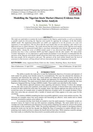
  • 6. Modelling the Nigerian Stock Market (Shars) Evidence from Time Series Analysis www.theijes.com The IJES Page 6 Figure (2.1a) (2.1 b) Quadratic model. The quadratic equation (see fig. 2.1b) is given as Y t =5410.78-176.236t+1.10268t2 .with a MAPE value of 344, a MAD value of 3772 and MSD value of 25521225. Figure (2.1b) (2.1 c) Exponential model The exponential equation (see fig.2.1c) is given as Yt=114.651(1.02281t ) with a MAPE value of 24, a MAD value of 2443 and MSD value of 321050434.
  • 7. Modelling the Nigerian Stock Market (Shars) Evidence from Time Series Analysis www.theijes.com The IJES Page 7 Figure (2.1c) (2.1 d) S-Curve. The S-Curve (peal fleed logistic) model (see fig.2.1d) is given as Yt=106 /(34.3832+12762.4(0.971699t )).with a MAPE value of 24, a MAD value of 3415 and MSD value of 6120008. Figure (2.1d) The graphs of the trend equations are shown in figures 2.1 (a), 2.1 (b), 2.1 (c) and 2.1 (d) above The error measures of the trend line equations are summarised in the table below: TREND MAPE MAD MSD Linear 885 6243 71991198 Quadratic 344 3772 25521225 Exponential 24 2443 32150434 S-curve (peal fleed logistic). 24 3415 61200108 Table 1.1
  • 8. Modelling the Nigerian Stock Market (Shars) Evidence from Time Series Analysis www.theijes.com The IJES Page 8 PERFORMANCE OF THE TREND LINE EQUATIONS As discussed earlier, an equation with minimum MAPE and MAD is considered to be a better trend or pattern. Among the models stated above, it could be seen that exponential model satisfies that condition and therefore could be selected as an appropriate trend or pattern for Nigeria Stock Exchange (shares). ADF Test Statistic -4.297321 1% Critical Value* -3.4552 5% Critical Value -2.8719 10% Critical Value -2.5723 *MacKinnon critical values for rejection of hypothesis of a unit root. Augmented Dickey-Fuller Test Equation Dependent Variable: D(SPR,2) Method: Least Squares Sample(adjusted): 1985:07 2008:12 Included observations: 282 after adjusting endpoints Variable Coefficient Std. Error t-Statistic Prob. D(SPR(-1)) -0.471422 0.109701 -4.297321 0.0000 D(SPR(-1),2) -0.341030 0.111876 -3.048276 0.0025 D(SPR(-2),2) -0.209103 0.112643 -1.856335 0.0645 D(SPR(-3),2) 0.028770 0.097721 0.294407 0.7687 D(SPR(-4),2) -0.054867 0.070278 -0.780721 0.4356 C 38.80649 80.64386 0.481208 0.6307 R-squared 0.428587 Mean dependent var -5.584291 Adjusted R-squared 0.418235 S.D. dependent var 1725.834 S.E. of regression 1316.354 Akaike info criterion 17.22417 Sum squared resid 4.78E+08 Schwarz criterion 17.30165 Log likelihood -2422.607 F-statistic 41.40263 Durbin-Watson stat 1.997573 Prob(F-statistic) 0.000000 Table 1.2 Figure. 2.2 plot of time series (Shares, 1985- 2008 ) Model 1: ARMA, using observations 1985:01-2008:12 (T = 288) Dependent variable: shares Standard errors based on Hessian
  • 9. Modelling the Nigerian Stock Market (Shars) Evidence from Time Series Analysis www.theijes.com The IJES Page 9 Coefficient Std. Error Z p-value Const 13341.2 11252.2 1.1857 0.23576 phi_1 0.994188 0.00516065 192.6479 <0.00001 *** theta_1 0.202119 0.0544073 3.7149 0.00020 *** Mean dependent var 10590.70 S.D. dependent var 14593.40 Mean of innovations 30.33702 S.D. of innovations 1358.582 Log-likelihood -2488.776 Akaike criterion 4985.551 Schwarz criterion 5000.203 Hannan-Quinn 4991.423 Real Imaginary Modulus Frequency AR Root 1 1.0058 0.0000 1.0058 0.0000 MA Root 1 -4.9476 0.0000 4.9476 0.5000 a -0.2 -0.15 -0.1 -0.05 0 0.05 0.1 0.15 0.2 0 5 10 15 20 25 lag Residual ACF +- 1.96/T^0.5 -0.2 -0.15 -0.1 -0.05 0 0.05 0.1 0.15 0.2 0 5 10 15 20 25 lag Residual PACF +- 1.96/T^0.5 fig.2.2 ACF AND PACF (Before differencing) Root 2 1.4960 0.0000 1.4960 0.0000 Model 2: ARIMA, using observations 1985:02-2008:12 (T = 287) Dependent variable: (1-L) shares Standard errors based on Hessian Coefficient Std. Error Z p-value Const 73.5225 179.985 0.4085 0.68291 phi_1 0.0980653 0.168414 0.5823 0.56037 phi_2 0.648896 0.133664 4.8547 <0.00001 *** theta_1 0.136203 0.164541 0.8278 0.40780 theta_2 -0.537849 0.107461 -5.0051 <0.00001 ***
  • 10. Modelling the Nigerian Stock Market (Shars) Evidence from Time Series Analysis www.theijes.com The IJES Page 10 Mean dependent var 109.1969 S.D. dependent var 1392.149 Mean of innovations -6.145163 S.D. of innovations 1311.197 Log-likelihood -2467.638 Akaike criterion 4947.277 Schwarz criterion 4969.234 Hannan-Quinn 4956.077 Real Imaginary Modulus Frequency AR Root 1 -1.3193 0.0000 1.3193 0.5000 Root 2 1.1681 0.0000 1.1681 0.0000 MA Root 1 -1.2428 0.0000 1.2428 0.5000 Root 2 1.4960 0.0000 1.4960 0.0000 Table 2.2 ACF -0.15 -0.1 -0.05 0 0.05 0.1 0.15 0 5 10 15 20 25 lag Residual ACF +- 1.96/T^0.5 -0.15 -0.1 -0.05 0 0.05 0.1 0.15 0 5 10 15 20 25 lag Residual PACF +- 1.96/T^0.5 Fig. 2.3 ACF AND PACF (after differencing) ARIMA (2 , 1,2) III. RESULTS FOR ARIMA MODELS. As discussed earlier in section 3.3.1 for ARIMA, model identification was performed first followed by model estimation. Let’s see the model identification step first. 3.1 Results for ARIMA Model identification. The model identification was performed using Autocorrelation Function (ACF) and Partial Autocorrelation function (PACF) plots (see appendix A for the details) Figure 2.2 shows the ACF and PACF for Nigeria Stock Exchange (shares) with d=0. The two lines parallel to X-axis show 95% confidence interval. Anything inside these lines can be treated as zero. In the figure, ACF plot doesn’t decay rapidly, which means that the series is non- stationary, hence needs differencing (according to rule 2 in appendixes A).
  • 11. Modelling the Nigerian Stock Market (Shars) Evidence from Time Series Analysis www.theijes.com The IJES Page 11 Figure 2.3 shows ACF and PACF plots for Nigeria Stock Exchange (shares). From ACF plot it is clear that there is no need of further differencing (according to rule 1 in appendix A). Here ACF and PACF both plots are mixtures of exponentials and damp sine waves, which start after the first lag. Hence according to rule 5 in appendix A, the model identified is ARIMA (2, 1 2). Also these plots resemble the pattern from region 4 in figure A.3 which ensures ARIMA (2, 1, 2) model. Also out of all the models that were tried, it was observed that ARIMA (2, 1, 2) model gave minimum MAPE (L), minimum MAE (L), (see table 2.2 above). Though, there is no need for further differencing, one more differencing was performed as the models with d=2 were also tested for forecasting in the next step of the experiment. Figures 2.3 show ACF and PACF plots for that. From the figures, PACF decays as good as exponentially, while ACF is nonzero till the second lag. Hence according to rule 4 in appendix A. ARIMA (0, 2,2.) may also be fit for this series. TABLE 3.1 DIFFERENT PERFORMANCES OF ARIMA MODELS P D Q MAPE MAE R.SQUARD S.R.SQUARED 1 1 1 11.501 531.342 992 109 1 0 1 54.116 592.110 989 989 1 1 0 15.053 543.121 991 062 2 0 1 46.979 581.849 991 991 2 0 0 51.026 580.637 989 989 2 1 0 13.515 536.155 992 089 1 0 0 50.542 608.584 988 988 0 1 2 16.959 557.028 992 059 1 0 2 52.018 581.807 989 989 0 1 0 22.486 605.063 991 008 0 1 1 18.904 559.879 991 049 1 1 2 11.983 543.333 992 113 2 1 1 12.109 540.740 992 112 2 0 2 55.170 601.811 989 989 2 1 2 10.500 529.615 992 112 0 2 0 8.931 605.103 992 001 1 2 0 7.965 601.725 990 237 2 2 0 11.019 592.228 991 368 2 2 2 11.622 576.596 992 404 1 2 2 9.509 548.510 992 394 0 2 2 11.014 563.556 992 392 2 2 1 11.341 573.065 395 395 1 2 1 10.990 562.487 992 392 0 2 1 10.881 556.222 992 392 0 0 2 488.732 3231.897 894 894 0 0 1 851.342. 5660.993 717 717 0 0 0 1572.863 10707.946 000 000 Conclusion and Recommendations From the experiments performed in this study, the following conclusions can be drawn. 1. Model identification indicated that ARIMA (2, 1, 2) is the best fit of this index. This was supported by the forecasting results of different ARIMA models as the forecasting performance of ARIMA (2, 1, 2) was better than other ARIMA models. 2. MA models (i.e. ARIMA with p = d = 0) and ARIMA models with d = 0 are not suitable for these series. 3. The experiment shows that exponential model gives the best trend line or pattern for Nigeria stock exchange as noticed in figure (4.1 c) which gives minimum value of MAPE and MAD. It was therefore recommended that the operators of the Nigerian stock market should relaxed the bottle necks and stringent laws on stock practices so that more people will be attracted to take part. The operators of the stock market should raise the level of awareness so that investors will keep abreast with new innovations and what is happening in the market.
  • 12. Modelling the Nigerian Stock Market (Shars) Evidence from Time Series Analysis www.theijes.com The IJES Page 12 REFERENCES [1]. Abhyankar, A. et al. (1997); the nature of Statistical learning Theory and Price indices. Introduction to stock Market prices in developing countries. [2]. Agrawalla, R.K. and Tureja, S.K. (2007), ‘causality between stock market development and economic growth: A case study of india’, journal of management research, 7,158- 169. [3]. Alex, J. S. and Bernhard S. (2004) A tutorial on support vector regression statistics and computing. . [4]. Alile , H. (1996),; Dismantling Barrier of foreign Capital flows. The Business Times of Nigeria 14th April, page 5. [5]. Arestis, P., Demetriades, P.O and Luintel, K. B (2001).’financial development and economic growth: the role of stock markets’ Journal of money, credit and Banking, 33, 16-41. [6]. Arief, S.(1995).Share price determination and share price behaviour in developing economies. The case study of Malaysia and Singapore, Sritua, Arief Associates, Jakarta. [7]. Atiya, A., Talaat, N, and Shahean, S.(1997). An efficient stock market forecasting, model using neural networks. Neural network International conference. [8]. Box, G.E. Jenkins, G.M. and Reinsel, G.C.(1994) Time series analysis, forecasting and control.. [9]. Brooks, R.D., Davidson, S. and Faff, R.W. (1997). ‘An examination of the effects of major political change on stock market volatility, the South African experience,’ journal of international financial Markets, institutions and money, vol 7(3), pp 255-275. [10]. Central Bank of Nigeria’s (CBN) Statistical Bulletin (Various issues). [11]. Chi- cheong, C. w.,Man- chung, C. and Chi- Chung, L. .(2000) Financial Time series forecasting by neural network using conjugate gradient learning algorithm and multiple linear regression weight initialization, computing in Economics and finance. [12]. Darrat, A. F. (2000) ‘On testing the Random walk Hypothesis. A model comparison approach, financial review, vol.35 no.3 pp105. [13]. Demirgue- Kunt, A. and Ross, L. (1996), ‘ Stock Market, corporate finance and Economic Growth; An overview’. The world Bank Review. Pg.223-239. [14]. Dickson, J.P. and Muragu K. (1994). Market Efficiency in developing countries. A case study of the Nairobi stock exchange’ Journal of Business Finance and Accounting, vol 21(1), pp 133- 150. [15]. Eugene, F. (1970), ‘Theory of Efficient Capital Markets’. In graduate school of Business. University of Chicago. [16]. Fama, E.(1994) The behaviour of stock market prices, in graduate school of Business, university of Chicago. [17]. Gidofalvi , G.(2001) using News articles to predict stock price movements,. University of California, San Diego, Department of computer science and Engineering. [18]. H. Roberts, (1999). ‘statistical versus clinical prediction of the stock market’.. [19]. H.F. Zou, G.P. Xia, F.T. Yang and H.Y. Wang.(2007) An investigation and comparison of artificial neural Network and time series Models for Chinese food grain price forecasting.. [20]. Habibullah, M.S. (1999), ‘financial development and economic growth in Asian countries: testing the financial – led growth hypothesis’, savings and development, 23,279- 290. [21]. Investopedia A Forbes media company.(2004). Efficient Market Hypothesis (EMH). In http//www.investopedia.com/terms/e/efficient market hypothesis. [22]. J. Zurada.(1994) , U.S.A Introduction to Artificial Neural Systems. [23]. Le Baron. (1999). Inefficient Market Hypothesis. Forecasting Financial Market using past prices to determine the present prices. [24]. Lijuan Cao and Francis E.H.Tay (2001). financial forecasting using support vector machines. Neural computing and applications. [25]. Lisa, B., Jeffery, J. and Choudary, R.H (1998) Improving forecasting for telemarketing centres by Arima modelling with intervention. International journal of forecasting