Six Myths about Ontologies: The Basics of Formal Ontology
Heteroskedasticity
1. Chapter 10: Heteroskedasticity
In this chapter:
1. Graphing to detect heteroskedasticity (UE 10.1)
2. Testing for heteroskedasticity: the Park test (UE 10.3.2)
3. Testing for heteroskedasticity: White's test (UE 10.3.3)
4. Remedies for heteroskedasticity: weighted least squares (UE 10.4.1)
5. Remedies for heteroskedasticity: heteroskedasticity corrected standard errors (UE
10.4.2)
6. Remedies for heteroskedasticity: redefining variables (UE 10.4.3)
7. Exercises
The petroleum consumption example specified in UE 10.5 will be used to demonstrate all
aspects of heteroskedasticity covered in this guide. Data for this problem is found in
EViews workfile named Gas10.wf1 and printed in Table 10.1 (UE, p. 371).
Graphing to detect heteroskedasticity (UE 10.1):
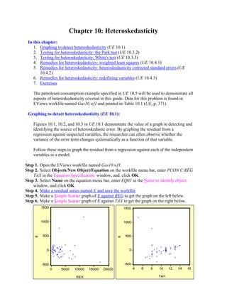
Figures 10.1, 10.2, and 10.3 in UE 10.1 demonstrate the value of a graph in detecting and
identifying the source of heteroskedastic error. By graphing the residual from a
regression against suspected variables, the researcher can often observe whether the
variance of the error term changes systematically as a function of that variable.
Follow these steps to graph the residual from a regression against each of the independent
variables in a model:
Step 1. Open the EViews workfile named Gas10.wf1.
Step 2. Select Objects/New Object/Equation on the workfile menu bar, enter PCON C REG
TAX in the Equation Specification: window, and. click OK.
Step 3. Select Name on the equation menu bar, enter EQ01 in the Name to identify object:
window, and click OK.
Step 4. Make a residual series named E and save the workfile.
Step 5. Make a Simple Scatter graph of E against REG to get the graph on the left below.
Step 6. Make a Simple Scatter graph of E against TAX to get the graph on the right below.
2. Testing for heteroskedasticity: the Park test (UE 10.3.2):
Complete Steps 1-3 of the section entitled Graphing to detect heteroskedasticity before
attempting this section. Follow these steps to complete the Park test for
heteroskedasticity:
Step 1. Open the EViews
workfile named Gas10.wf1.
Step 2. Select Objects/New
Object/Equation on the
workfile menu bar, enter
log(E^2) C log(REG) in the
Equation Specification:
window, and click OK to
reveal the EViews output on
the right.
Step 3. Test the significance of
the coefficient on log(REG).
Testing for heteroskedasticity: White's test (UE 10.3.3 & UE, Equation 10.12):
Complete Steps 1-3 of the section entitled Graphing to detect heteroskedasticity before
attempting this section. Follow these steps to complete White's test for heteroskedasticity:
Step 1. Open the EViews workfile
named Gas10.wf1.
Step 2. Select Objects/New
Object/Equation on the
workfile menu bar and enter
PCON C REG TAX in the
Equation Specification:
window. Click OK.
Step 3. To carry out White’s
heteroskedasticity test for
the regression in Step 2,
select View/Residual
Tests/White
Heteroskedasticity (cross
terms) to get the output on
the right. EViews reports
two test statistics from the
test regression. The Obs*R-
squared statistic highlighted
in yellow and boxed in red,
is White’s test statistic. It is
computed as the number of
3. observations (n) times the R2 from the test regression. White’s test statistic is
asymptotically distributed as a χ2 with degrees of freedom equal to the number of slope
coefficients, excluding the constant, in the test regression (five in this example).
Step 4. The critical χ2 value can be calculated in EViews by typing the following formula in
the EViews command window: =@qchisq(.95,5).1 After typing the formula and hitting
Enter on the keyboard, appears in the lower left of the EViews
screen (the same value found in UE, Table B-8). Since the nR2 value of 33.2256393731 is
greater than the 5% critical χ2 value of 11.0704976935, we can reject the null hypothesis
of no heteroskedasticity. The probability printed to the right of the nR2 value in the
EViews output for White’s heteroskedasticity test (i.e., 0.000003) represents the
probability that you would be incorrect if you rejected the null hypothesis of no
heteroskedasticity.2 The F-statistic is an omitted variable test for the joint significance of
all cross products, excluding the constant. It is printed above White's test statistic for
comparison purposes.
Remedies for heteroskedasticity: weighted least squares (UE 10.4.1):
Follow these steps to estimate the weighted least squares using REG as the
proportionality factor:
Step 1. Open the EViews
workfile named
Gas10.wf1.
Step 2. Select Objects/New
Object/Equation on
the workfile menu bar,
enter PCON/REG
1/REG REG/REG
TAX/REG in the
Equation
Specification:
window, and click
OK. Note the
coefficients
highlighted in yellow.
1
c=@qchisq(p,v) calculates the percentile of the χ2 distribution . The formula finds the value c such that
the prob(χ2 with v degrees of freedom is ≤ c) = p. In this case, the prob(χ2 with 5 degrees of freedom is ≤
11.0704976935) =95%. In other words, 95% of the area of a χ2 distribution, with v=5 degrees of freedom,
is in the range from 0 to 11.0704976935 and 5% is in the range from 11.0704976935 to ∞ (in the tail).
2
The probability value is calculated with the formula =@chisq(x,v), which returns the probability that a
chi-squared statistic with v degrees of freedom exceeds x. To verify this, type the formula
=@chisq(33.2256393731,5) in the EViews command window and read the value of 3.39442964858e-06 on
the lower left of the EViews screen.
4. Step 3. Select Objects/New
Object/Equation on the
workfile menu bar and
enter PCON C REG TAX
in the Equation
Specification: window,
and select the O Options
button (see the arrow
pointing toward the red
box area in the graphic
on the right).
Step 4. Check the Weighted
LS/TSLS box and enter 1/REG in the
Weight: window (see the yellow
highlighted and red boxed areas in the
graphic on the right).
Step 5. Select OK to accept the options and
select OK again to estimate the equation.
Note that the weighted least squares
coefficients found in Step 2 are the same
as the coefficients found in Step 5 using
the EViews weighted least squares
option.3
3
EViews performs weighted least squares by first dividing the weight series by its mean, then multiplying
all of the data for each observation by the scaled weight series. The scaling of the weight series is a
normalization that has no effect on the parameter results, but makes the weighted residuals more
comparable to the un-weighted residuals. The normalization does imply, however, that EViews weighted
least squares is not appropriate in situations where the scale of the weight series is relevant, as in frequency
weighting.
5. Remedies for heteroskedasticity: heteroskedasticity corrected standard errors (UE
10.4.2):
Follow these steps to estimate heteroskedasticity corrected standard errors regression:
Step 1. Open the EViews workfile named Gas10.wf1.
Step 2. Select Objects/New Object/Equation on the workfile menu bar and enter PCON C
REG TAX in the Equation Specification: window, and select the O Options button.
Step 3. Check the Heteroskedasticity
Consistent Covariances (White)
box (see the yellow highlighted and
red boxed areas in the graphic on the
right).
Step 4. Select OK to accept the options
and select OK again to estimate the
equation.
Step 5. Compare the Estimation Output
from the regression with the
Heteroskedasticity Consistent
Covariance on the lower left with the
Estimation Output from the
uncorrected OLS regression on the
lower right (EQ01). Note that the
coefficients are the same but the
uncorrected std. error is smaller. This means that the Heteroskedasticity Consistent
Covariance correction has reduced the size of the t-statistics for the coefficients, a typical
result. However, in this case both of the slope coefficients remain significant at the 5%
level but the TAX variable coefficient is no longer significant at the 1% level.
6. Remedies for heteroskedasticity: redefining variables (UE 10.4.3):
Follow these steps to estimate UE, Equation 10.30, p. 374:
Step 1. Open the EViews workfile named Gas10.wf1.
Step 2. Select Objects/New Object/Equation on the workfile menu bar, enter PCON/POP C
REG/POP TAX in the Equation Specification: window, and click OK.
Exercises:
5. Create an EViews workfile and enter the average income and average consumption
data from the table printed in Exercise 5, p.378.
a. Refer to Testing for heteroskedasticity: the Park test.
b. Refer to Testing for heteroskedasticity: the Park test.
c.
d. Refer to Remedies for heteroskedasticity: heteroskedasticity corrected standard
errors.
9. Open the EViews file named Books10.wf1.
a.
b.
c. Refer to Testing for heteroskedasticity: the Park test and Testing for
heteroskedasticity: White's test.
d. Refer to Remedies for heteroskedasticity: weighted least squares.
e. Refer to Remedies for heteroskedasticity: heteroskedasticity corrected standard
errors or Remedies for heteroskedasticity: redefining variables.
15. Open the EViews file named Bid10.wf1.
a. Refer to Estimate a multiple regression model using EViews and Serial
Correlation (Chapter 9).
b. Refer to Serial Correlation (Chapter 9).
c.
d. Refer to Testing for heteroskedasticity: the Park test and Testing for
heteroskedasticity: White's test.
e. Refer to Testing for heteroskedasticity: the Park test and Testing for
heteroskedasticity: White's test.
f.