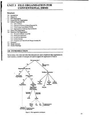
1. UNIT 3 FILE ORGANISATION FOR
CONVENTIONAL DBMS
Structure
3.0 Inuoduction
3.1 Objectives
3.2 File Organisation
3.3 Sequential File Organisation
3.4 Indexed Sequential File
3.4.1 Types of Indexes
3.4.2 Organisation Structure of Indexed Sequentid file
3.4.3 Vinual Storage Amsr Method (VSAM)
3.4.4 Implementation of Indexing using tree Svufuare
3.5 Direct File Organisation
3.6 Multi-ke y File Organisation
3.6.1 The need for Multiple Accus Path
3.6.2 Multilist file Organisdon
3.6.3 lnvened File manisation
3.6.4 Cellular Partitions
3.6.5 Comparison and Trade-off in the Design of muhikey file
I 3.7 Summary
3.8 'Model Answers
3.9 Further Readings
I
3.0 INTRODUCTION
i
I Just as arrays, lists, uees and other data structures are used to implement clata organisation in
main memory, a number of strategies are used to supporr the organisation of data in
Sequent+l Direct access
Orgclnrsabon only ?
file
Strudure Structure
Orgi&ati on Ring file
I (Sequential +
I Direct Access)
. I !Eg T!w Tk } mtmnim
Implementation
Tree
Hashing
mechanism

2. Intruluctury Concepts of
Data B.a Mmagcmcnt System secondary memory. In this unit we will look at different strategies of organizing data in the
secondary memory. In this unit, we are concerned with obtaining data representation for files
on external storage devices so that required functions (e.g. retrieval, update) may be carried
out efficiently. The particular organisation most suitable for any application will depend
upon such factors as the kind of external storage available, types of queries allowed, number
of keys, mode of retrieval and mode of update. The figure 1 illustrates different file
organisations based on an access key.
3.1 OBJECTIVES
After going through this unit you will be able to:
define what is a file organisation
list file organisation techniques
discuss implementation techniques of indexing through tree-structure
discuss implementation of direct file organisation
discuss implementation of multikey file organisation
discuss trade-off and comparison among file organisation techniques
3.2 FILE ORGANISATION
Precise definition of each of these technique will be presented later in this unit.
The technique used to represent and store the records on a file is called the file organisation.
The four fundamental file organisation techniques that we will discuss are the following:
1. Sequential
2. Relative
3. Indexed sequential
4. Multi-key
, >
There are two basic ways, that the file organisation techniques differ. First, the organkition
determines the tile's record sequencing, which is the physical ordering of the records in
storage.
Second, the file organisation determines the set of operation necessary to find particular
records. Individual records are typically identified by having particular values in search-key
fields. This data field may or may not have duplicate values in file, the field can be a group
or elementary item. Some file organisation techniques provide rapid akcessibility on a variety
of search key; other techniques support direct access only on the value of a single one.
The organisation most appropriate for a particular file is determined by the operational
characteristics of the storage medium used an the nature of the operations to be performed on
the data. The most important characteristic of a storage device that influences selection of a
storage device once the appropriate file organisation technique has been determined) is
whether the device allows direct access to particular record occurrences without accessing
all physically prior record occurrences that are stored on the device, or allows only
sequential access to record occurrences. Magnetic disks are examples of direct access
storage devices (abbreviated DASD's); magnetic tapes are examples of sequential storage
devices.
3.3 SEOUENTIAL FILE ORGANISATION
The most basic way to organise the collection of records that from a file is to use sequential
organisation. In a sequentially organised file records are written consecutively when the file
is created and must be accessed consecutively when the file is later used for input (figure 2).

3. Mle Org~tionFu r
Conventional DBMS
Begnning of
File
Record 2
1 Record n-1 I 1 Record N I
In a sequential file, records are maintained in the logical sequence of their primary key
values. The processing of a sequential file is conceptually simple but inefficient for random
access. However, if access to the file is strictly sequential, a sequential file is suitable. A
sequential file could be stQ.ed on a sequential storage &vice such as a magnetic tape. I Search for a given record in a sequential file requires, on average, access to half the records
in the file. Consider a system where the file is stored on a direct access device such as a disk.
Suppose the key value is sepamted from the rest of the record and a pointer is used to
indicate the location of the record. In such a system, the device may scan over the ke values
at rotation speeds and only read in the desired record. A binary or logarithmic semh I'
technique may also be used to search for a record. In this method, the cylinder on which the
required record is stored is located by a series of decreasing head movements. The search,
having been localised to a cylinder, may require the reading of half the tracks, on average, in
the case where keys are embedded in the physical records, or require only a scan over the
tracks in the case where keys are also stored separately. I Updating usually requires the creation of a new file. To maintain file sequence, records are
copied to the point where amendment is required. The changes are then made and copied into
the new file. Following this, the remaining records in the original file are copied to the new
file. This method of updating a sequential file creates an automatic backup copy. It permits
updates of the type U, through U,. , t Addition can be handled in a manner similar to updating. Adding a record necessitates the
shifting of all records hm the appropriate point to the end of file to create space for the new
record. Inversely, deletion of a record requires a compression of the file space, achieved by
the shifting of records. Changes to an existing record may also require shifting if the record
size expands or shrinks. I The basic advantage offered by a sequential file is the ease of access to the next record, the
simplicity of organisation and the absence of auxiliary data structures. However, replies to .
simple queries are time consuming for large files. Updates, as seen above,'usually require the
creation of a new file. A single update is an expensive proposition if a new file must be
created. To reduce the cost per update, all such requests are batched, sorted in the order of the
sequential file, and then used to update the sequential file in a single pass. Such a file,
containing the updates to be made to a sequential file, is sometimes referred to a transaction
In the batched mode of updating, a transaction file of update records is made and then sorted
in the sequence of the sequential file. The update process requires the examination of each
individual record in the original sequential file (the old master file). qecords requiring no
changes are copied directly to a new fde (the new master file); records requiring one or
more changes are written into the new master file only after all necessary changes have been
made. Insertions of new records are made in the proper sequence. They are written into the
new master file at the appropriate place. Records to be deleted are not copied to the new
master fde. A big advantage of this method of update is the creation of an automatic backup
copy. The new master file can always be recreated by processing the old master fde and the

4. Intruductory Cvncuptv ul
Data Bar Managemerrt Systern
I I I
Block, Block, Block,
Figure 3 : A We 4th empty spaces for record insertions
A possible method of reducing the creation of a new file at each update run is to create the
original file with "holes" (space left for the addition of new records, as shown in the last
figure). As such, if a block could hold K records, then at initial creation it is made to contain
only L * K records, where 0 < L I 1 is known as the loading factor. Additional space may
also be earmarked for records that may "overflow" their blocks, e.g., if the record ri logically
belongs to block Bi but the physical block Bi does not contain the requisite free space. This
additional free space is known as the overflow area. A similar technique is employed in
index-sequential files.
3.4 INDEX-SEQUENTIAL FILE ORGANISATION
The retrieval of a record from a sequential file, on average, requires access to half the records
in the file, making such enquiries not only ineff~cienbt ut very time consuming for large files.
To improve the query response time of a sequential file, a type of indexing technique can be
added.
An index is a set of y, address pairs. Indexing associates a set of objects to a set of orderable
quantities, which are usually smaller in number or their properties provide a mechanism for
faster search. The purpose of indexing is to expedite the search process. Indexes created from
a sequential (or sorted) set of primary keys are referred to as index sequential. Although the
indices and the data blocks are held together physically, we distinguish between them
logically. We shall use the term index file to describe the indexes and data file to refer to the
data records. The index is usually small enough to be read into the processor memory.
A sequential (or sorted on primary keys) file that is indexed is called an index sequential
file. The index provides for random access to records, while the sequential nature of the file
provides easy access to the subsequent records as well as sequential processing. An
additional feature of this file system is the overflow area. This feature provides additional
space for record addition without necessitating the creation of a new file. Before starting
discussion on index sequential file suucture, let us, discuss types of indexes.
3.4.1 Types of Indexes
The idea behind an index xcess suucture is similar to that behind the indexes used
commonly in textbooks. A textbook index lists important terms at the end of the book in
alphabetic order. Along with each term, a list of page numbers where the term appears is
given. We can sekh the index to find a list of addresses - page numbers in this case - and
use these addresses to locate the tcrm in the textbook by searching the specified pages. The
alternative, if no other guidance is given, is to sift slowly through the whole textbooks word
by word to find the term we are interested in, which corresponds to doing a linear search on a
file. Of course, most books do have additional information. such as chapter and section titles.
which can help us find a term without having to search through the whole book. However.
the index is the only exact indication of where each term occurs in the book.
An index is usually defined on a single field of a file, called an indexing field. The index
typically stores each value of the index field along with a list of pointers to all disk blocks
that contain a record with that iield valuc. The values in the index are ordered so that we can
do a binary search on the index. The index file is much smaller than rhe data file, so
searching the index using binary search is reasonably efficient. Multilevel indexing does
away with the need for binary search at the expense of creating indexes to the index itself!
There are several types of indexcs. A primary index is an index specified on the ordering
key field of an ordered file of recortls. Recall lhat an ordering key field is used to physically
order the file records on disk, and evcry record has a unique value for that field. If the

5. ordering field is not a kcy field that is, several records in te file can have the same value for
the ordering field another type of index, called a clustering index, can be used. Notice that a
file can have at most one physical ordering field, so it can have at most one primary index or
one clustering index, but not both. A third type of index, called a secondary index, can be
specified on any nonordering field of a file. A file can have several secondary indexes in
addition to its primary access method. In the next three subsections we discuss these three
types of indexes.
Primary Indexes
A primary index is an ordered file whose records are of fixed length with two fields. The
fust field is of the same data types as the ordering key field of the data file, and the second
field is a pointer to a disk blokc - a block address. The ordering key field is called thc
primary key of the data fileThere is one index entry (or index record) in the index file for
each block in the dam file. Each index errtry has the value of the primary key field for the
fust record in a block and a pointer to other block as its two field values. We will refer to the
two field values of index entry i as K(i), P(i).
To create a primary index on the ordered file shown in fiugre 4, we use the Name field as the
primary key. because that is the ordering key field fo the file (assuming that each value of
NAME SSN BIRTHDATE JOB SALARY SEX
block 1 'Aaron, Ed
Abbon. Diane I
Acosta. Marc 1
Mock 2
block 4
Adams. John I
Adams, Robin I
Akers. an- I
block 3
block 5
Alexander. Ed (
Alfred. Bob I 1 1 1
block 6
block n
Allen. Sam 1
Allen. Troy I
anders. Keith 1 1
Anderson, Rob (
Anderson, Zach I
Angeli. Joe 1
Archer. Sue I
1
Arnoid. Mack I
Flle Organlsncloa For
Conventlond DBMS
1
Arnold. Steven I
Atkins. Timothy 1
Wong, James I
Woods. Manny (
I
1 1
Zimmer. Byron I
figure 4 : Some blocks cn an ordered (sequential) file of EM PLOY EE mcords with NAME af the ordcrinp fldd

6. Introductory Conaepts of NAME is unique). Each entry in the index will have a NAME value and a pointer. The first
Data Bam Mmqmment System three index enhies would be:
cK(1) = (Aaron, Ed), P(l)= address of block 1>
cK(2) = (Adams. John), P(l) = address of block 2 >
cK(3) = (A1exander.E.). P(3) = address of block 3>
(a) NAME SSN JOB
2
3
(b) dam fields overflow pdnter
- null pointer = -1
- overflow pointer refers to position of
next record in linked list
Fipre 5 : IUustrPtlng Internal bashing data shuclures
0
1
-1
M It
(a) Amy of M positloas for use In hashing. @) Collision resdutlon by chdning of records.
Figure 6 illustrates this primary index. The total number of entries in the index will be the
same as the number of disk blocks in the ordered data file. The fust record in each block of
the data file is called the anchor record of the block, or simply the block anchor (a scheme
similar to the one described here can be used, with the last record in each block, rather than
the first, as the block anchor. A primary index is an example of what is called a nondense
index because it includes an entry for each disk block of the data file mther than for eveq
record in the data fde. A dense index. on the other hand, contains an entry for every record in
the file.
The index file far a primary indexjneeds substantially fewer blocks than the data file for two
reasons. First, there are fewer index entries than there are records in tk data file because an
entry exists f& each whole block of the data file rather than for each mord. Second..each
index entry is typically smaller in size than a data record because it ha only two fields, so

7. more index entries than data records will fit in one block. A binary search on the index file He 0rgdatio11 Fnr
will hence require fewer block accesses than a binary search on the data file. Conventional DBMS
DATA FILE
&PR IMARY Y FIELD)
NAME SSN BIRTHDATE X>B SALARY SEX
Aaron. Ed
Abbon. Diane I
Acosta, Marc 1 I I I
Adams,John 1 1 I I
INDEX FILE Adams. Robin I
(aK(i), P(I)> enttiee)
Akers. Jan I I I I I
- . -, Anderson, Sach I
Anderson. Rob 1 I I Arnold. Mack
.Anderson. Zach [ I
Angeli, Joe I
Arnold. Mack 1 1
Arnold. Steven 1 I 1
Atkins. Timothy 1 I I I
Wong. James I
Wood, Donald 1 I
Wright. Pam 1
Wyan. Charles I
[~mmerB. yron I I
Figure 6 : Ribnary index on the ordering key field of the file shown in riure 5
A record whose primarykey value is K will be in the block whose address is P(i), where
Ki I K I (i + 1). The ilk block in the data file contains all such records because of the
physical ordering of the file records on the primary key field, we do a binary search on the
index file to find the apppriate index entry i, then remeve the data file block whose address
is P(i). Notice that the atove formula would not be correct if the data file was ordered on a
nonkey field that allowsmultiple records to have the same ordering field value. In that case
the same index value as that in the block anchor could be repeated in the last records of the
previous block. Example 1 illustrates the saving in block accesses when using an index to
search for a record.
Example 1 : Suppose w have an ordered file with r = 30,000 records stored on a disk with
block size B = 1024 bytes. File records are of fixed size and unspanned with record.length R
= 100 bytes. The blocking factor for the file would be bfr L(B/R)J = L(IM~/Ioo)J = 10
records per block. The mmber of blocks needed for the file is b = r(rlbfr)l = r(30,~/10)1=

8. Intnductary ConapU of
Data BPL Management Syatem
3000 blocks. A binary search.on the data file would need approximately r(log2b)l =
r(log,3~)i = 12 block accesses.
Now suppose the ordering key field of the file is V = 9 bytes long, a block pointer is P= 6
bytes long, and we conshuct a primary index for the file. The size of each index enuy is Ri =
(9 + 6) = 15 bytes, so the blocking factor for the index is bfr, = L(B/R)J = L (102~115)J = 68
entries per block.
The total number of index entries ri is equal to the number of blocks in the data file, which is
3000. The number of blocks needcd for the index is hence bi = r
blocks. To perform a binary search on the index file would need
block accesses. To search for a record using the index, we need
to the data file for a total of 6 + 1 = 7 block accesses - an improvement over binary search on
the data file, which required 12 block accesses.
A major problem with a primary index - as with any ordered file - is insertion and deletion of
records. With a primary index, the problem is compounded because if we attempt to insert a
record in its correct position in the data file, we not only have to move records to make space
for the new record but also have to change some index entries because moving records will
change the anchor recd of some blocks. We can use an unordered ovefflow file. Another
possibility is to use a linked list of overflow records for each block in the data file. We can
keep the records within eech block and its overflow linked list sorted to improve retrieval
time. Record deletion can be handled using deletion markers.
Clustering Indexes
If records of a file are physically ordered on a nonkey field that does not have a distinct value
for each record, that field is called the clustering field of the file. We can create a different
type of index, called a clustering index, to speed up remeval of records that have the same
DATA FlLE
(CLUSTERING
FIELD)
DEPTNUMBER NAW SSN .DB BIRTHDATE SALARY
I
1
NDEX FILE 1
(<K(I), PO)+ @dm) I
2
CLUSTERING
3
VALUE WtNER 3
~&rc7 :A dusterlag index on the DEPFNUMBER addngM do frn EMPLOYEE file

9. value lor the clustering field. This differs from a primary index, which requires that the
ordering field of the data file have a distinct value for each record.
A clustering index is also an ordered file with two fields; the first field is of the same type as
the clustering field of the data file and the second field is a block pointer. There is one entry
in the clustering index for each distinct value of the clustering field, containing that value
and a pointer to the first block in the data file that has a record with that value for its
DATA FlLE
(CLUSTERING
FIELD)
MPTNUMBER NAME SSN JOB BIRTHDATE SALARY
1
1
1
block pointer nu1 pointer
-- --
block pointer nu1 pointer
nu1 pointer
INDEX FlLE
(<K(I). P(I)> entries)
VALUE POINTER I
block pointer nu1 pointer
I Fly
BL~K-~. block po~nter nu1 pointer
CLUSTFRING
4
5
6 5
8 5
5
5
block pointer nu1 pointer
I 6
block winter nu1 pointer
File OrgnnisPtion Fnr '
Conventloanl DBMS
4
block pointer nu1 pointer
Rpre 8 : Clustering index with separate blocks for each group d records
with the same value for the clustering lleld

10. Introductory Conepts d
Data Bosc Management System
clustering field. Figure 7 shows an example of a data file with a clustering index. Note the
record insertion and record deletion still cause considerable problems because the data
records are physically ordered. To alleviate the problem of insertion, it is common to reserve
a whole block for each value of the clustering field; all records with that value are placed in
the block. If more than one block is needed to store the records for a particular value,
additional blocks are allocated and linked together. This makes inseation and deletion
relatively strpightforward. Figure 8 shows this scheme.
A clustering index is another example of a nondense index because it has an entry forevery
distinct value of the indexing field rather than for evrey record in the file.
Secondary Indexes
A secondary index also is an ordered file with two fields, and, as in the other indexes, the
second field is a pointer to a disk block. The first field is of the same data type as some
nonordering field of the data file. The field on which the secondary index is constructed is
called an indexing field of the file. whether its values are distinct for every record or not.
There can be many secondary indexes, and hence indexing fields, for the same file.
We first consider a secondary index on a key field - a field having a distinct value for every
record in the data file. Such a field is sometimes called a secondary key for the file. In this
case there is one index entry for each record in the data file, which has the value of the
secondary key for the record and a pointer to the block in which the record is stored. A
secondary index on a key field is a dense index because it contains one entry for each record
in the data file.
We again refer to the two field values of index enby i as K(i), P(i). The entries are ordered
by value of K(i), so we can use binary search on the index. Because the records of the data
file are not physically ordered by values of the seq~daryke y field, we cannot use block
INDEX FlLE
(<K(I), P(I)> entries) DATA FILE
INDEXING
FIELD
INDEX (SECONDARY
KEY FIELD)
Figure 9 : Adense secondary Index on a nonordering key field of a fUe

11. anchors. Thatls why an index entry is created for each record in the data file rather than for
each block as in the case of a primary index. Figure 9 illustrates a secondary index on a key
attribute of a data file. Notice that in figure 9 the pointers P(i) in the index entries are block
pointers, not record pointers. Once the appropriate block is transferred to main memory, a
search for the desired record within the block can be carried out.
A secondary index will usualy need substantially more storage space than a primary index
becaue of its larger number of entries. However, the improvement in search time for an
arbitrary record is much greater for a secondary index than it is for a primary index, because
we would have to do a linear search on the data file if the secondary indcx did not exist. For
a primary index, we could still use binary search on the main file even if the index did not
exist because the records are physically ordcred by the primary key field. Example 2
illustrates the improvement in number of blocks accessed when using a secondary index to
search for a record.
Example 2 : Consider the file of Example I with r = 30,000'fixed- length records of sizc R =
100 bytes stored on a disk with block size B = 1024 bytes. The file has b = 3000 blocks as
calculated in Example 1. To do a linear search on the file, we would require bl2 = 3000/2 =
1500 block accesses on the average.
Suppose we construct a secondary index on a nonordering kcy ficld of the file that is V = 9
bytes long. As in Example 1, a block pointer is P = 6 bytes long, so each index entry is R. =
(9 + 6 ) = 15 bytes, and the blocking factor for thc index is bfri = L(B/R,)I = L(1024115)J =
68 entries per block. In a dense secondary index such as this, the total numbcr of index
entries is ri is equal to the number of records in the data file, which is 30,000. The number of
blocks needed for the index is hence bi = (ri/bfri) = (30,000168) = 442 blocks.
Compare this to the 45 blocks needed by the nondensc primary index in Example 1.
A binary search on this secondary index qeeds (log?bj) = (log,442) = 9 block accesses. To
search Tor a record using the index, we need an additlonal block access to thc data file for a
total of 9 + 1 = 10 block acccsscs - a vast improvement ovcr the 1500 block accesscs needed
on the averagc for a linear search.
Figure 10 : A secondary lhdex on a nonkey fidd implemented using one level of indirectinn so that index •
entries are fled length and have unique field values
File Orgdsation For
ConvenUonal DBMS

12. Introductory Concepts of We can also create a secondary index on a nonkey field of a file. In this case numerous
Data records in the &ta file can have the same value for the indexing field. There are several
options for implementing such an index:
Option 1 is to include several index entries with the same K(i) value - one for each
record. This would be a dense index.
Option 2 is to have variable-length records for the index entries, with a repeating
field for the painter. We keep a list of pointers (i.1). ....,P( iJr) in the indexentry for
K(i) - one pointer to each block that contains a record whose indexing field value
equals K(i). In either option 1 or option 2, the binary search algorithm on the index
must be modified appropriately.
Option 3, which is used commonly, is to keep the index entries themselves at a
fixed length and have a single entry f a each index field value, but create an extra
level of indirection to handle the multiple pointers. In this scheme, which is
nondense, the ponter P(i) in index entry (i), P(i) points to a block of record pointers;
each record pointer in that block points to one of the data file reords with a value
K(i) for the indexing field. If some value K(i) has too many records, so that their
record pointers cannot fit in a single disk block, a linked list of blocks can be used.
This technique is illustrated in figure 10. Retrieval via the index requires an
additiond block access because of the extra level, but the algorithms for searching
the index and, more important, for insertion of new records in the data file are
straightforward. In addition, retrievals on complex selection conditions may be
handled by rofemng to the pointers without having to retrieve many unnecessary
file records.
Notice that a secondary index provides a logical ordering on the records by the indexing
field. If we access the records in order of the entries in the secondary index, we get them in
order of the indexing field.
Multilevel Indexing Schemes : Basic Technique
In a full indexing scheme, the address of every record is maintained in the index. For a small
file, this index would be small and can be processed cry efficiently in main memory. For a
Pointer Pointer
to next to next Pointer
Key level Key level Key to
index index record
Pointer
Key tonext
~ndex
Highest level
index
Intermediate
level indexes
Figure 11 : Hierarchy of indexes
Lowest
level index

13. large tile, the index's size would pose problems. It is possible to create a hierarchy of indexes FUC org.ldsslion FO~
with the lowest level index pointing to the records, while the higher level indexes point to the CoavLntk3.l DBMS
indexes below them (figure 11). The higher level indices are small and can be moved to main
memory, allowing the search to be localised to one of the larger lower level indices.
The lowest level index consists of the <key, address> pair for each record in the file; this is
costly in terms of space. Updates of records require changes to the index file as well as the
data file. Insertion of a record requires that its &y, address> pair be inserted in the index at
the correct point, while deletion of a record requires that the <key, address> pair be removed
from the index. Thexefore, maintenance of the index is also expensive. In the simplest case,
updates of variable length records require that changes be made to the address f~lodf the
record entry. In a variation of this scheme, the address value in the lowest level index entry
points to a block of records and the key value represents the highest key value of recods in
this block. Another variation of this scheme is described in the next section.
3.4.2 Structure of Index Sequential Files
An index-sequential file consists of the data plus one or more levels of indexes. When
inserting a record, we have to maintain the sequence of records and this may necessitate
shifting subsequent records. For a large file this is a costly and inefficient process. Instead.
the records that overflow their logical area are shifted into a designated overflow area and a
pointer is provided in the logical area or associated index entry points to the overflow
location. This is illustrated below (figure 12). Record 165 is inserted in the original logical
block causing a record to be moved to an overflow block.
Original logical Modc
1 611 i 812 1 614 / 615 j 618
611 ,i
Original logical Mock ~vefiow~ odc
Figure 12 : Overflow of record
Multiple records belonging to the same logical area may be chained to maintained logical
sequencing. When records are forced into the overflow areas as a result of insertion, the
insertion process is simplified, but the search time is increased. Deletion of records from
index-sequential files creates logical gaps; the records are not physically removed but only
flagged as having been deleted. If there were a number of deletions, we may have a great
amount of unused space.
An index-sequential file is therefore made up of the following components:
1. A primary data storage area. In certain systems this area may have unused spaces
embedded within it to permit addition of records. It may also include records that have
been marked as having been deleted.
2. Overflow area(s). This permits the addition of records to the files. A number of schemes
exist for the incorporation of records in these areas into the expected logical sequence.
3. A hierarcy of indices. In a random enquiry or update, the physical location of the desired
record is obrained by accessing these indices.
The primary data area contains the records written by the users' programs. The records are
written in data blocks in ascending key sequence. These data blocks are in turn stored in
ascending sequence in the primary data area. The data blocks ate sequenced by the highest
key of the logical records contained in them.
There are several approaches to structuring both the index and sequential data portion of an
indexed sequential file. The most common approach is to build the index as a me of key
values. The tree is typicaly a variation on B-tree which we will discuss later. The other
common approach is to build the index based on the physical layout of the data in storage.
The important technique for building index based on the physical layout of the data in
storage is ISAM (Index sequential access method) which we will discuss.

14. Introductory Concepts of
Data Base Management System
Physical Data Organisation Under ISAM
When a record is stored by ISAM, its record key must be one of the fields in the record. The
records themselves are first sorted by record key into ascending order before they are stored
on one or more disk drives. ISAM will always maintain the records in this sorted order. Each
record is stored on one of the tracks of a disk. Those records that follow it in sorted sequence
are placed directly after it on the same track or, if room does not permit, are spilled over onto
the next track in the same cylinder. In other words, they are dropped down to the next platter
surface. The ann does not move; looking downwared, the next head is selected eletronically.
Since the tracks on a cylinder are labelled 0, 1,2, ......... the records that follow those on track
1 are placed on track 2. Track 0 is the next file cylinder. The cylinders are also labelled 0, 1,
2, . . . . .
Figure 13 shows two cylinders of records, but only their keys are shown. Note that the keys
are in ascending sequence throughout their storage on both cylinders. We have not shown
record 0 on either cylinder, as this is used by ISAM for control. Of course, the number of
tracks on each cylinder is a function of the size of the disk pack.
When ISAM retrieves a record, it needs to know the cylinder, the track address, and the
record key. These are the components that must make up the directory entries for the ISAM
file. In ISAM a directory is called an index. For example, if a directory entry for record 1500
gave cylinder 9 and track 3, then ISAM would select cylinder 9. The read head associated
with track 3 would then be activated. The bottom side of the top platter is usually track 0
because the top being exposed is subject to damage; therefore, the read head selected would
be that for the top side of the third platter, as shown in figure 14. Of course, the required
record might be one of the many records stored on track 3. Rotation of the drive would
eventually bring the required record under the read head. The desired record is identified by
its record key.
Because the records in an ISAM file are kept in sorted order by record key, it is not necessaq
to have a directory entry for every single record. It is sufficient to know the largest record
key on every track of te file. For example, suppose the largest key on the track 3 is 100 atid
the largest on track 4 is 200. A record with key 175, if it exists in the file at all, must be on
track 4. It cannot be on track 3 as the largest key on that track is 100.
The most obvious place to keep the directory for each cylinder on the file is, of course, on
the cylinder itself, and it is on track 0 of each cylinder that ISAM keeps its directory. This
directory is known as a track index; it contains the largest key on every track and the
hardware address of that track. Figure 15 shows a typical track index for one cylinder of a
file. In this cylinder, for example, 400 is shown to be the largest key on track 3 and 700 the
largest key on the cylinder. Later we will see that this directory is slightly more complicated.
This will be clarified when we discuss how ISAM keeps track of records that are added to
Track
Flgure 13 : Record Storage

15. - -
the file after its original creation. For the moment, this simplified version of the directory is FLle Organisation For
Conventional DBMS
more than sufficient
Cylinder 0
Cylinder 1 3GD Cylinder 2
(a) (b)
Figure 14 : Di% organbation (a) dWr; @) top view ofplatter
1 150 2 200 .3 400' ... ... 20 700
k track key track key track key track key
Figure 15 : 'hack Index
How does the ISAM use this directory to find a record on the file? First it positions the
readwrite mechanism over the appropriate cylinder and selects track 0. Let us suppose that
the index on track 0 has the entries shown below in figure 15 and the systcm seeks the key
350. The entry indicates that the record, if it is to be found, will be on track 3. The read head
for track 3 is selected and the rotation of the drive will eventually bring the record with key
350, if it exists, under this read head. The fact that the index for this cylinder is on the
cylinder itself means that no additional movement of the readlwrite mechanism is necessary.
Wac k key
When an ISAM file ip spread over several cylinders, there is more than one track index. A
track index is placed on track 0 of each cylinder used by the file. There remains then in this
case a further problem. When a record is being sought, which track index should be
examined? Not surprisingly, ISAM keeps a cylinder index with an entry for each of its track
indexes. Each entry in this index specifies the address of every track index and the largest
entry in each track index. In other words, the cylinder index has an entry for each cylinder of
the file and the largest entry on that cylinder. The following is a typical cylinder index:
cyl key cyl key cyl key cyl key
This cylinder index shows that on cylinder 15 the largest key that will be found is 2000. If
ISAM is seekylg record 1886, an examination of this cylinder index reveals that the record,
if it exists, can be found on cylinder 15. The read/write mechanism moves to cylinder 15,
selects track 0, and consults the track index. If that track index is then track 2 is selected.
track key track key uack key
The cylinder index is not associatkd with any particular cylinder of the file and is stored in a
separate area or on another disk altogether. This are is referred to as the cylinder area. The
file itself along with the track indexes is called the primearea.

16. lolmductory Colroepts d
Dst. BuM m~qommSt yacm
Sometimes a file may be very large, even extending across several disk drives. In this case
hundreds of cylinders may be involved causing the cylinder index itself to be several tracks
or cylinders in size. In this eventuality, ISAM may even create an index of the cylinder
index. Such an index is called a master index. Each entry of the master index then points to a
track of the cylinder index and specifies the largest key given on this track of the cylinder
index. Even another master index might be made of this index. Perhaps now the reader can
I appreciate why the name "Indexed" is the first word in ISAM.
Figure 16 shows segments of each of the three types of indexes. The reader should try to
follow the search dgaithm, beginning at the master index, for the location ot recam 43.
Only two tracks of both the master index and cylinder index are shown. The first entry in the
master index says that the largest key mentioned in track 1 of the cylinder index is 211. The
first entry on track 1 of the cylinder index shows that 95 is the west key on the track index
on cylinder 6. Checking the track index of cylinder 6 shows that record 45 is located on track
2. Record 45 also happens to be the largest record key on track 2.
Cylinder index I
H .C 6 I 1 I T2r5a c1k 2 i nId 4ex5 fo1 r tracks 121 0-21 09 5 I - %
0
Flpre 16 : Send algorithm through three hdexea Overflow Records In JSAM
Overflow Records in ISAM
Unlike Relative 1-0, which does not permit the addition of a new record to a file unless an
empty slot is available. ISAM allows any number of new records to be added to an existing
file. The number is limited by the availability of sufficient storage sphce. As mentioned
earlier, ISAM also maintains the original ordering of the sorted file. Any record to be added
is inserted into the file a an appopriate place. To accomplish this insertion. room must be
made available for the record on its track by shifting each record that logically follows the
one to be added forward on the uack and dropping the last record on the Vack off the end
For example. if the records ht the end of a track are
and record 34 is to be added, then the track will be changed to
and record 37 will be dropped off the end. The track's highest key is now 35 and the track
index is changed accordingly. The question. of course, is what to do with record 37 that was
dropped. If it is added to the next uack, it will cause the record at the end of that track to be
dropped off the end and a domino effect will cascade through all the records on the file. In
each case, the track index will need to be changed as will the cylinder index when the last
record on the cylinder is forced off. To avoid this problem, the record dropped off the
original track is removed from the file and placed in an overflow area. This overflow area
may be on another disk unit, elsewhere on the same disk unit, or even perhaps on the same
cylinder if several tracks on each cylinder are set aside and designated for overflow use. The
exact placement of the overflow area is determined when space for the file is requested from
the operating system.

17. Earlier, it was noted that a simplified version of the track index had been presented. This
version can now be upgraded. In actual fact, there are two entries for each track on a given
cylinder. We shall designate them as " N and "0 entries, where " N denotes a normal entry
and "0" an overflow entry. Before overflow records are added to the file, both entries are the
same. For example, the track index for cylinder 6 of a file might appear as
In this case, both the N and 0 entries for track 2 designate that 200 is the largest key on this
track. Suppose, in fact, that track 2 contains the following records (only the keys shown):
As indicated by the track index, the largest key to be found on track 2 is 200. Now suppose
. record 185 is to be added to this track forcing record 200 off the end into the overflow area.
Track 2 now becomes
As the largest key on track 2 is now 190, the N entry for this track in the index must be
t changed to 190 as follows:
N 0 N 0 N
Suppose further that record 200 is placed in an overflow area on track 10 and is the fust
record on this overflow track. If this is designated as 10: 1, the overflow area should be
changed as follows:
In effect, then, record 200 has become the fust of many possible records in the overflow
area.
If record 186 is added to track 2, forcing 190 off the end into the overflow area leaving track I 2as
!
I. then record 190 will be added as the second record in the overflow area, namely 10:2, and
the overflow entry on the track index will be replaced by 10:2 so that the track index
becomes
File Organisation For
Conventional DBMS
Note that in the 0 entry the 200 is not changed as it still represents the largest record key in
the overflow area. In fact the previous entry 10: 1 is added to the latest record to be added to
the overflow area, record 190, so that it is not lost The overflow area now looks like
with record 190 pointing to record 200. The symbol "#" indicates that record 200 does not
point to another record. The overflow entry always contains two values :
Wrepresents the largest key value in the overflow area that has been moved there from an
individual track (200 in the above example) and the other contains a pointer to the smallest
key in the overflow area (190 in the above example). If record 194 is now spilled to the
overflow area, the 0 entry will not be changed as 190 is still the smallest record key value in

18. Introductory Concepts of
Data Base Management System
the overflow am. As the record with key 194 comes after 190, record 190 is adjusted to
point to record 194 and 194 to 200. The sorted order is maintained in the overlow area,
which now appears as
It is not necessary that the records stored on a track in the overflow area be associated with
only one track of the prime area. This is only the case here because we have assumed that all
the overflow records on track 10 come from track 2. This is not always so. It is quite possible
to have overflow records from many other tracks so that we could well imagine an overflow
area as follows:
where records 214 and 216 have arrived from track 4. Record 214 is the second overflow
record from track 4 and points to the first from track 4, namely 216, at location 10:3.
The algorithm to be employed in adding a record to the overflow area can now be stated:
ALGORITHM : OVERFLOW ADDITIONS
1. Find the first available position in the overflow area.
2. Move the record to this position
3. If this record is the record of lowest key in the overflow area, place the pointer to this
record in the overflow entry of the track index and move the old value in the track index
to the pointer field of the newly added record. If this is not the case, move the address of
the new record to the pointer field of the record in the overflow area that precedes it in
sorted sequence and place the old value of the pointer into the pointer field of the new
record.
Overflow Considerations
If a record is in the prime area df a file, its retrieval is straightforward. The master, cylidner.
and track indexes are examined1 the appropriate track selected; and finally. after rotational
delay of the drive, the record is retrieved. This is not true if the record is in the overflow area.
If the record is in the overflow area, its retrieval can rake a long time. Suppose, for example.
that record 16.000 is the first record moved to an overflow area and later followed by 60
more such records. As these 60 later records are chained together in key sequence order by
pointer. all 60 records will have to read before record 16.000 can be located. As each read is
a timeconsuming process, this can take a lon time. the efficiency of ISAM is defeated by
allowing large numbers of records to overflow from a single track.
This problem can be overcome by writing a "clean-up" program which reads all the records
on the file, including those in the overflow areas and creates a larger file. This can be done
whenever the time taken to retrieve records has become unacceptable. The time taken for
retrieval is the dominant criterion here as it is acceptable to have a large overflow area
if the records in it are seldom retrieved.
The other possibility is. as with relative files to create dummy records. In ISAM a dummy
record is a record that contains HIGH-VALUES in the first character position but must, as
with all records in ISAM. also contain a unique key. During file creation these records are
sorted along with all the other file records and scattered whereever desired within the file.
Dummy records prevent growth in the overflow area in two ways. First, if a record to be
added to an ISAM file has the same key as a dummy record, it merely replaces the dummy
record. This is the ideal situation as no records are shifted along a given track and none of the
indexes are changed. The second feature of dumm y records is that they are not moved to the
overflow area if they are forced off the end of the track by the insertion of a new record.
They are simply ignored. The N entry in the track index is changed to reflect the fact that a
different record now holds the last position on the track. If both the 0 and N keys are the
same before the addition takes place, then they are both changed. Suppose, for example, that
the N and 0 entreis for track 7 of a certain cylinder are given as

19. File Organisation Fur
Cunvention;ll DBMS
and that track 7 has the keys
with record 100 being a dummy record. The addition of record 55 would change track 7 as
follows:
and since record 100 is a dummy record (and therefore not transferred to the overflow area),
the N and 0 enuies become
Creating an ISAM File
An ISAM file must be loaded sequentially in sorted order by record key. ISAM will detect a
record out of order. Any dummy records to be added to the file should be placed in the input
data stream in sequence. These records are best added where record additions are expected to
take place. For instance, a credit card company may expect in the near future to add records
whose keys range between 416-250-000 and 416-275-000 as a new district of credit card
holders is opened up. In this case, dummy records with these keys can be created and added
to the file during file creation. Another possibility is simply to scatter a certain percentage of
dummy records throughout the file. This is not nearly as effective nor alway possible (there
may be no unused keys in the file). Recall that a dummy record is only ignored if it is at the
end of a track. It will stay on a track until it is replaced by a valid record with the same key
or pushed off the end by a new insertion.
Once the file is in use, any record whose deletion is desired can be turned into a dummy
record by writing HIGH-VALUES in its first character position. This is a useful feature,
especially in a credit card situation or phone number list where inactive customers can be
replaced.
So what is he significance of the ISAM organisation ?
Advantages of ISAM indexes :
1) Because the whole sructure is ordered to a large extent, partial (LIKE ty%) and range
(BETWEEN 12 and 18) based retrievals can often benefit from the use of this type of
index.
2) ISAM is good for static tables becasue there are usually fewer index levels than B-tree.
3) Because the Index is never updated, there are never any locking contention problems
within the index itself-this can occur in B-tree indexes, especially when they get to the
point of 'splitting' to create another level.
4) In general there are fewer disk VOs required to access data, provided there is no overflow.
5) Again if little overflow is evident, then data tends to be clustered. This means that a
single block retrieval often brings back rows with similar key values and of relevance to
the initiating query.
Disadvantages of ISAM indexes :
1) ISAM is still not as quick as some (hash okanisation, dealt with later, is quicker).
2) Overflow can be a real problem in highly volatile tables.
3) The sparse index means that the lowest level of index has only the highest key' for a
specific data page, and therefore the block (or more usually a block header), must be
scarched to locate specific rows in a block.

20. Introductory Concepts of
Data Base Management System In a nutshell therefore, these are the two types of indexing generally available. As I have
already said, indexes can be either created on one single, or several groups. of columns
within single tables, and generally the ability to create them should be a privilege under the
control of the DBA. Indexes usually take up significant disk space, and although generally of
significant benefit in the case of data retrieval, they can slow down insedupdate and delete
operation because of overhead in maintaining the index, and in ISAM of ensuring the logical
organisation of the data rows. The presence of an index does not mean that the RDBMS will
always use it, a reality of life disc&sed later; and it is also true that it is not genemlly
possible to pick and choose which index will be used under which conditions. If follows.
therefore, that the adminismation of indexes should be done centrally, with great case, and
should be a major consideration in the physical design stage of a project due to its
application dependence.
Before leaving these types of access mechanisms and moving on to an explanation of
hashing, it is worth listing some of the other functions that may be required within the
context of manipulating indexes.
3.4.3 VSAM
The major disadvantage of the index-sequential organisation is that as the file grows.
performance deteriorates rapidly because of overflows and consequently there arises the
need for periodic reorganisation. Reorganisation is an expensive process and the file
becomes unavailable during reorganisation. The virtual storage access method
(VSAM) is IBM's advanced version of the index-sequential organisation that avoids
these disadvantages. The system is immune to the characteristics of the storage medium,
which could be considered as a pool of blocks. The VSAM files are made up of two
components: the index and data. However, unlikq index-sequential organisation,
overflows are handled in a different manner. The VSAM index and data are assigned to
distinct blocks of virtual storage called a control interval. To allow for growth, each
time a data block overflows it is divided into two blocks and appropriate changes are
made to the indexes to reflect this division.
3.4.4 Implementation of Indexing throu~hT ree-Structure
Indexes support applications that selectively access individual records, rather than searching
through the entire collection in sequence. One field (or a group of fields) is used as the index
field. For example in a banking application, there might be a file of records describing
Branch Offtces. It might be appropriate to index the file on Branch Name, providing access
to Branch Office information to support interactive inquiries.
We shall start with a relatively simple tree-structured index and then progress to more
complex structures.
Binary Search Trees As Indexes
Let us first reconsider the binary semh tree. Recall that the nodes of a binary search tree are
arranged in such a way that a search for a particular key value proceeds down one bmnch of
the tree. The sought key value is compared with the key value of the tree's root: if it is less
than the root value, the search proceeds down the left subtree; if it is greater than the mot
value, the search proceeds down the right subtree. The same logic is applied at each node
encountered until the search is satisfied or it is determined that the sought key is not included
in the tree.
Typically, a key value does not stand alone. Rather, the key value is associated with
information fields to form a record. In general, storing these information fields in the binary
search tree would make for a very large tree. In order to speed searches and to reduce the
tree size, the information fields of records commonly are stored separate from the key
values. These records are organised into files and are sotred on secondary storage devices
such as rotating disks. The connection between a key value in the binary search tee and the
corresponding record in the file is made by housing a pointer to the record with the key
value.
Figure 17 shows the binary search tree with pointers included to the data records.

21. mELEMENT
L
Figure 17 : Binary search trec from figure 8-23 used as an index
This augmentation of the binary search tree to include pointers (i.e. addresses) to data
records outside the structure qualifies the tree to be an index. An index is a structured
collection of key value and address pairs; the primary purpose of an index is to facilitate
access to a collection of records. An index is said to be a dense index if it contains a key
value-address pair for each record in the collection. An index that is not dense is sometimes
called a sparse index. There are many ways to-organise an index; the augmented binary
search tree is one approach.
At this time we will not concern ourselves with the actual location of those records on
primary or secondary storage. Suffice it to say that in contrast to relative files where the
physical locations of records are determined by a hash algorithm applied to key valucs, thcre
is significantly more frccdom in the physical placement of records in an indexed lllc.
M-Way Search Trees
The performance of an index can be enhanced significanlly by incrcasing the branching
factor of the wee. Rather than binary branching, m-way (m2) branch~ngc an be used. For
expository purposes, wc ignore for the moment pointers out of the structure to data records
and consider only the internal structure of the wee. An m-way search tree is a tree in which
each node has out- degree <= m. When an m-way search tree is not empty, it has the
following properties.
1. Each node of the tree has the structure shown in figure 18.
I'iyre 18 : Fundamental structure of a nodein an m-way search tree
The Po, P,, ........., Pn are pointers to the node's subtrees and the KO, ......, K,., are key values.
The requirement that each node have out-degree <= m forces n = m-1.
2. The kcy valucs in a node are in ascending order:
KI < K1+1
for i = 0, ..... n-2.
3. All key values in nodes of the subtree pointed lo by P, are less than the key value K, for i
=0, ......., n-I.
4. All key valucs in nodes of the subwee pointed to by Pn are greatcr than the key value
Kn-1.
5. The subtrees pointed to by the PI, i = 0, ......., n arc also m-way search trccs.
Note that the arrangement of key values in nodes is analogous to their arrangement in
binary scarch trees. A five-way search tree has a maximum of five pointers oul of each
node, i.e., n 4. Some nodes of the wee may conhin fewer than fivc poinlers.

22. Introductory Concepts of
Data Base Management System Examyle
Figure 19 illustrates a three-way search tree. Only the key values and the non-null subtree
pointers are shown. In the figure, leaf nodes have been depicted as containing just key
values. Each internal node of the search tree has the structure depicted in figure 18, here with
a maximum of three subtree pointers.
Figure 19 : Example three-way search tree
M-Way Search lkees as Indexes
When an m-way search tree is used as an index, each key- pointer pair (K, Pi) becomes a
triplet Pi, Ki, Ai where Ai is the address of the data record associated with key value K,. Thus,
each tree node not only points to its child nodes in the tree, but also points into the collection
of data records. If the index is dense, every record in the collection will be pointed to by
some node in the index.
We can define the node type for an m-way search tree index as follows in Pascal.
nodeptr = ? nodetype;
recptr = ? rectype;
n 1, keytype = integer;
nodetype = record
n:integer
keypus:- [O..n I ] of record
pU ) nodepu;
ke) '1 key type;
adw : Wptr
end;
keyptrn:nod=
end;
Again key's typeyd not be integer, n I m - 1 and nl = n - 1.
Searching an M-Way Search Tree
The process of searching for a key value in an m-way search tree is a relatively
straightforward extension of the process of searching for a key value in a binary search tree.
A recursive version of the search aIgorithm follows. The variablekeys cdntains the sought
key value; r initially points to the root of the tree. The search tree is assumed to be global,
with -var -nod e: nodetype
procedure search(skey ;keytrype;s cnodeptr, f0undrec:recptr);
-var i ;O..n;
-if (r=mJ
then foundrec: =
-else b egin i: = 0;
-while ( i < n @ skey node.key[i])
-do i:=i+l;
-if (i < n and skey = node.key[i])
then foundrec : = node.addrl:i]
-el-se if i < n
-then s earch (skey,node.ptr[i],foundrec)
-else s earch(skey,node.keyptm,foundrec)
end;
-end;

23. Compare this logic with direct searches of a binary search tree. The primary difference is that
the array of keys in each node of the m-way tree must be scanned to find the appropriate
pointcr to follow either down to a child node or directly to the data record.
B-TREES
The basic B-tree structure was discovered by R.Bayer and E. McCreight (1970) of Boeing
Scientific Research Labs and has grown to become one of the most popular techniques for
organising an index structure. Many variations on the basic B-tree have been developed; we
cover the basic structure fmt and then introduce some of the variations.
The B-tree is known as the balanced sort tree, which is useful for external sorting. There are
strong uses of B-trees in a database system as pointed out by D.Corner (1979) : "While no
single scheme can be optimum for all applications, the technique of organising a file and its
index called the B-uee is, de facto, the standard organisation for indexes in a database system."
The file is a collection of records. The index refers to a unique key, associated with each
record. One application of B- trees is found in IBM's Virtual Storage Access Method
(VSAM) file organisation. Many data manipulation tasks require data storage only in main
memory. For applications with a large database running on a system with limited company.
the data must be stored as records on secondary memory (disks) and be accessed in pieces.
The size of a record can be quite large, as shown below:
struc t DATA
I
int ssn;
char name [80];
char address 1801;
char schoold [76];
struct DATA * left; /* main memory addresses */
slruct DATA * right; I* main memory addresses *I
d-block d-left; I* disk block address *I
d-block d-right; I* disk block address */
1
There are two sets of pointers in the struct DATA. The main memory pointers, left and right,
are used when the children of the node are in memory and the disk addresses, d-left and
d-right, are used to reference the children on the disk. The size of DATA is 256 bytes.
Data is moved by block msfer into main memory for manipulation; however, the disk
access is slow (tens of milliseconds) compared with a main memory move (tens of
microseconds), so we want to minimise the disk accesses. One method is to make the data
nodes even fractions (1I2,1/4, etc. or multiples (1.2, etc.) of the disk sector size.
Another method is to expand the capacity of the node for storage of data. A binary tree node
contains one key or data element and has pointers to two children. We can construct a tree
with nodes that have more than two possible children and more than one key. The tree has a
I property called order, the maximum number of children.,for any given node. If the maximum
is N children, then the order of the tree is N.
The ADT B-Tree
To reduce disk accesses, several conditions of the tree must be true; the height of the tree
must be kept to a minimum; there must be no empty sublrees above the leaves of the tree; the
leaves of the tree must all be on the same level; and all nodes except the leaves must have at
. least some minimum number of children @haps half of the maximum). The toot alone may have no children, if the tree has only one node. Otherwise it may have as few as two and as
many as the maximum number of children. The keys in the tree should have some defined
ordering (numerical, lexical, or some other relationship). A,tree that has these properties is
called a balanced sort tree (a B-tree). The B-tree properties are listed below.
An ADT B-Tree of order N is a tree in which:
1. Each node has a maximum of N children and a minimum of NI2 children. The root may
have no children or any number from 2 to the maximum.
2. Each node has one fewer keys than children with a maximum of N- 1 keys.
3. the keys are arranged in a defined order within the node. All keys in the subtree to the
left of a key are predecessors of the key, and all keys in the subtree tothe right of a key
are successors of the key.
File Organisation For
Conventional DBMS -.

24. Introductory Concepts of 4. When a new key is to be inserted into a fullnode, the node is split into two nodes, and
Data Base Management System the key with the median value is inserted in the parent node. In case the parent node is
the root, a new root node is created.
5. All leaves are on the same level. There is no empty subtree above the level of the leaves.
Insertion in the B-Tree
The insertion of a new key into a B-tree begins with the search for a match. If a match is
found for the key, then the insertion operation takes some action (an error message is sent or
a count is incremented, etc.) and returns an error indication to the caller. If no match is found,
then the key is simply added to a leaf, unless the left is ful. If the leaf is full then it is split
into two nodes (requiring creation of a new node and the copying of half of the old nodes
keys and pointers to the new node) and the median value key is inserted into the parent of the
node. If the parent was also full, the split and key push up ripples upward. The ordering of
the keys is maintained, and the ordering of keys among subtrees is maintained.
The tree trends to become more balanced with subsequent insertions. The B-tree is like a
crystal in its growth: upward and outward from its base, the leaf level. To illustrate the
insertion process, we will build a B-tree of order 5 by inserting the following data:
The key ordering is ascending lexical. We keep track of the pointers by numbering them.
D. First the root node is created (+), then key D is inserted into it.
H, K, Z: the keys are searched for match; if match not found, they are simply inserted.
B: The nodc is full, so it must be split; of the keys, B, D, H, K, and Z, key H is the median
value key, so it promotes to the parent, but this is the root node so we must create a new node (+).
P, Q, E, A: Each key is simply inserted.
S: The node is full, so it must be split. A new node at the leaf level is created (*). Of the keys.
K, P, Q, S, and Z, key Q is the median value.

25. 1 h, T: Thc keys arc simply inserted.
C: The nodc is full, so it must bc split. A new node at thc leaf lcvcl is crcatcd (*). OC hc kcys,
A, B, C, D, and E, key C is hc mcdian valuc.
L, N: The keys arc simply inscrtca.
Y: Thc ntxlc is full, so it must be split. A new node a1 ~hIcca f lcvcl is crated (*). Of die
kcys, S, T, W, Y, and 2, key W is the mcxiian valuc.
h.1: The nodc is lull, so it must. bc split. A new notlc at thc lcaC lcvcl is crcatcd (*). OC hc
kcys, K, L, bl, N, and P, kcy M is thc ~nctlianv aluc.

26. Introductory Concepts of
Data Base Management System The root node is also full, so it is split. A new root node is created (+). Of the keys, C, H, M,
Q, and W, the key M is the median key. It is inserted into the new root.
Note how the balance has been maintained thmghout the insertions. A node split prepares the
way for a number of simple inseh. If the number of keys in a node is large, the time before
the next split (involving node &on and data transfer into the new node) will be fairly long.
Deletion of a Node in the B-'he
Deletion of a key is somewhhat the reverse of insertion. If the key is found in a leaf, the
deletion is fairly straightforward. If the key is not in a leaf, then the key's successor or
predecessor must be in a leaf, because the iyedon is done starting at a leaf. If the leaf is
full, the median value key is pushed upward, so the key closest in value to a key in a nonleaf
node must be in the root. The requirement that there be a minimum number of keys in a node
also plays a part, as we shall see.
If the key is found in a leaf node and the node has more than the minimum number of nodes,
then the key is simply deleted and the other keys in the node adjusted in position. If the node
has only the minimum number of keys, then we must look at the immediately adjacent leaf
nodes. If one of nodes has more than the minimum number of keys, the mdeian key in the
parent node is moved down to replace the deleted key and one of the keys from the adjacent
leaf node is moved into the parent node in place of the median key.
To demonstrale this deletion, we use the B-tree of order 5 shown in the section on insertion.
We will delete the key P from the tree after the insertion of the key S.
RIts leaf node is at minimum key count, and the adjacent node with keys A, B, D, and E has
more than the minimum key count. We can replace P with the median key H in the parent
node. We then replace H with the key closest to it in value, key E
If both of the adjacent n@es have only the minimum number of keys, one of the adjacent
nodes can be combined with the node that held the deleted key, and the median key from the
parent node that partitioned the two leaf nodes is pushed down into the new leaf node. We
will use the tree from the last example with keys A and B deleted.

27. File Org&.rtion For
Cooventinlral VRUS
P:lts leaf node is at minimum key count, and the adjacent nodes also have minimum key
count. We push H down into the combined node.
We summarise the key features of a B-tree as follows:
1. There is no redundant storage of search key values. That is, B-tree stores each search
key value in only one node, which may contain other search key values.
2. The B-tree is inherently balanced, and is ordered by only one type of search key.
3. The insertion and delction operations are complex with the time complexity OOog, n).
4. The search time is O(log2 n).
5. The number of keys in the nodes is not always the same. The storage management is
only complicated if you choose to create more space for pointers dnd keys, otherwise the
size of a node is fixed.
6. The B-tree grows at the'node as opposed to the binary tree, BST, and AVL trees.
7. For a B-tree of order N with n nodes, the height is log n. The height of a B-me increases
only because of a split at the root node.
There are several variations of B-tree, including B+ -tree and B* -tree. The B+ -tree indices
are similar to B-tree indices. The main difference between the Bt -tree and B-tree are:
1. In a B' - tree, the search keys are stored twice; each of the search keys is found in some
leaf nodes.
2. In a B-tree, there is no redundancy in storing search-kcy values; the search key is round
only one in the tree. Since search-key values that are found in nonleaf nodes are not
found anywhere else in the B-tree, an additional pointer field for each search key is kcpt
in a nonleaf node.
3. In a B+ -tree, the insertion and deletion operations are complex and O(log2 n), but the
search operation is simple, efficient, and O(log, n).
Because this B-tree structure is so common place, it is worth simply listing some of the more
imporlaln advantages and disadvantages.
Advantages of Btree indexes :
1) Because there is no overflow problem inherent wilh this type of organisation it is good
for dynamic table - those that suffer a great deal of insert / update /delete activity.
2) Bccause it is to a large extent sclf-maintaining, it is good in supporting %-hour operation.
3) As data is retrieved via the index it is always presented in ordcr.
4) 'Get next' queries are efficient because of the inherent ordering of rows within the index
blocks.
5) Btree indexes are good for very large tables because they will need minimal
reorganisation.

28. Intrcductory Concvptq of 6) Thcrc is prcdiclable acccss tinc r any wri ;x,al (of hc sarnc number of rows of coursc) Data Ilasc hanagemcnt System
bccausc thc Blrcc structurc kccps i&clf balanced, so that there is always the samc
number of indcx lcvcls for cvcb rclricval. Bear in mind of course, that thc nurnbcr of
indcx lcvcls docs incrcasc both with thc nurnbcr of records and the lcngth of Lhc kcy
valuc.
Bccausc thc rows arc in ordcr, this typc of indcx can scrvicc rangc typc cnquirics, of thc typc
bclow, cfficicntly.
SELECT ... WHERE COL BETWEEN X AND Y.
Disadvantages of Wee indexes :
1) For static tables, thcrc arc bcttcr organisations that rcquirc fcwcr 110s. ISAM indcxes arc
prcfcrablc to Blrcc in this typc of cnvironmcnt.
2) Blrcc is not rcally appropriate for vcry small tablcs bccausc indcx look-up bccomcs a
signilica~ipt an of hc ovcrall acccss timc.
3) Thc indcx can usc corisidcrablc disk space, cspccially in producls which allow dirfcrent
uscrs to crcalc scparatc indcxcs on thc samc tablclcolumn combinations.
4) Becausc thc indcxcs rhcrnsclvcs are subjcct to modification whcn rows arc updatcd,
dclctcd or inscrtcd, hcy arc also subjcct to locking which can inhibit concurrcncy.
So to concludc this section on Blrcc indcxcs, it is worth slrcssing that this structurc is by far
and away thc most popular, and pcrhaps vcrsatilc, of indcx slructurcs supported in thc world
of thc RDBMS today. Whilst not fully opti~niscdf or ccrlain activity, it is sccn as thc bca
singlc compromise in satislying all thc diffcrcnt acccss n~cthtxlsli kcly to bc rcquircd in
normal day-to-(fay opcration.
3.5 DIRECT FILE ORGANISATION
In thc indcx-scqucntial filc organisation considcrcd in thc prcvious sections, thc nlapping
from thc smrch-kcy valuc to thc storagc location is via indcx cntrics. In dircct filc
Kcy valuc - Addrcss
I:igure 20 : Mappir~g from a key value to an address valuc 4
organisation, thc kcy valuc is mappcd dircctly to thc storigc location. Thc usual mcthod of
dircct mapping is by performing somc arith~ncticm anipulation of thc kcy valuc. This proccss
is callcd hashing. Lct us considcr a hash function h Uiat maps thc kcy valuc k to thc valuc 4
h(k). Thc valuc h(k) is uscd as an adtlrcss and for our application wc rcquirc that this valuc
bc in solnc rangc. If our atltlrcss arca for thc rccords lics bctwccn S, and S2, thc rcquircrncnt
for thc hash function h(k) is that for all valucs of k it should gcncratc valucs bctwccn S, and
ST
It is obvious that a hash function that maps many diffcrcnt kcy valucs to a singlc addrcss or
onc that tltxs not rnap thc kcy valucs uniformly is a bad hash function. A collision is said to
occur whcn two tlistinct kcy valucs arc mappcct to thc sarnc storagc location. Collision is
hantllcd in a nirmbcr of ways. Thc colliding rccords may bc assigned to Lhc ncxt avpilablc
spacc, or thcy may bc assigned to an ovcrllow arca. Wc can i~n~ncdialclsyc c that with
hashing schcmcs thcrc arc no indcxcs to lravcrsc. With wcll-dcsigncd hashing fi~nclions
whcrc collisions arc fcw, this is a grcat advantage.
Anothcr problcm Uiat wc havc to rcsolvc is to dccidc what addrcss is rcprcscntcd by h(k). Lct
thc addrcsscs gc~icratcdb y thc hash function thc adtlrcsscs of buckcts in which thc y, atltlrcss
pair valucs of records arc storcd. Figurc shows thc buckcu containing thc y, adtlrcss pairs
that allow a rcorganisation or thc actual data rilc and actual rccord addrcss without alTccting
thc hash functions. A limited nurnbcr of collisions could bc hantllcd auto~naticallyb y thc usc
of a buckct of sulTicicnt capacity. Obviously thc spacc rcquircd for thc buckc~w ill bc, in
gcncral, much smallcr than thc actual (lala filc. Conscqucntly, i~r?co rganisation will not bc
that cxpcnsivc. Oncc tlic buckct ndtlrcss is gcncratcd from thc kcy by thc hash function, a

29. search in thc bucket is also rcct11;:cd lo locat ., ~lcldrcsso f ~hrcc quircd rccord. Howcvcr,
sirlcc the buckct sizc i.. .,111a1tlh, is ovcrhad is small.
The use of thc buckct ruluccs lhc problcm associalcd with collisions. In spilc of this, a
I)ucka may bccotnc full and thc resulting ovcrllow could bc handlcd by providing ovcrllow
huckcls ;ill(! using a pointcr from Ihc normal buckcl lo an cnlry in Ihc ovcrflow buckcl. All
such o!crl'low cnlrics arc linkcd. Multiplc ovcrllow from thc samc buckcl rcsulls in a long
list and slows down thc rctricval 'of thcsc rccords. In an altcrnalc schctne, Ihe addrcss
gcnccilcd by thc hash function is a buckct addrcss and Ihc buckct is usd to slorc Ihc records
tlircclly inslcad 01' using a pointcr to thc block containing thc rccord.
kcy addrcss I
12igurc 21: lluckct and bluck organisatitm fur hashing
Lcl s rcprcscnt thc valuc:
s = uppcr buckcl addrcss valuc - lowcr buckcl addrcss valuc + 1
Hcrc, s givcs thc numbcr of buckcls. Assumc Ihal wc havc somc mechanism lo convert key
valucs to nu~ncrico ncs. Thcn a sitnplc hashing function is:
h(k) = k mod s
whcrc k is lhc nutncric rcprcscnlalion of lhc key and h(k) produccs a buckcl addrcss. A
n~orncnl's thought lclls us lhal his mcthod would pcrlorm wcll in somc cascs and no1 in
others.
It has Ixcn showr~h, owcvcr, that thc choicc of a primc number for s is usually satisfactory. A
conr binalion of nlulliplicalivc and divisivc mcthods can be uscd lo advanlagc in many
pctctical silualions.

30. Introductory Concepts of '
Data Base Management System There are innumerable ways of convcrting a key to a numeric value. Most keys are numeric,
others may be either alphabetic or alphanumeric. In the latter two cases. we can use the bit
rep-i&tion of the alphabet to the numeric equivalent key. A number of simple
hashing methods are given below. Many hashing functions can be devised from these and
other ways.
1. Use the low order part of the key. For keys that are consecutive integers with few gaps,
this method can be used to map the keys to the available range.
2. End folding. For long keys, we identify start, middle, and end regions, such that the sum
of the lengths of the start and end regions equals the length of the middle region. The
start and end digits are cdncatenated and the concatenated suing of difits is added to the
middle region digits. This new number, mod s where s is the upper limit of the hash
function, gives the bucket address:
For the above key (converted to integer value if required) the end folding gives the two
values to be added as: 123456654321 and 123456789012.
3. Square all or part of the key and take a pari from the result. The whole or some defined
part of the key is squared and a number of digits are selccted from the square as being
part of the hash result. A variation is the multiplicative scheme where one part of the key
is multiplied by the remaining part and a numebr of digits are selected from the result.
4. Division. As stated in the beginning of this section, the key can be divided by a number,
usually a prime, and the remainder is taken as the bucket address. A simple check with,
for instance, a divisor of 100 tells us that the last two digits of any key will remain
unchanged. In applications where keys may be in some multiples, this would produce a
poor result. Therefore, division by a prime number is recommended. For many
applications, division by odd numbers that have no divisors less than about 19 gives
satisfactory results.
We can conclude from the above discussion that a number of possible methods for
generating a hash function exist. In general it has been found that hash functions using
division or multiplication performs quite well under most conditions.
To summarise the advantages and disadvantages of this approach :
Advantages of hashing :
1) Exact key matches are extremely quick.
2) Hashing is very good for long keys, or those with multiple columns, provided the
complete key value is provided for the query.
3) This organisation usually allows for the allocation of disk space so a good deal of disk
management is possible.
4) No disk space is used by this indexing method.
Disadvantages of hashing :
1) It becomes difficult to prcdict overflow because the workings of the hashing algorithm
will not be visible to the DBA.
2) No sorting of dam occurs either physically or logically so sequential access is poor,
3) This organisation usually takes a lot of disk space to ensure that no overflow occurs -
there is a plus side to this though: no space is wasted on index structures because they
simply don't exist.
To sum up hashing it's true to say that not many products support this type of suucutre, and it
is likely, I feel, to become entirely redundant in most software RDBMSs. In a hashing
organisation, the key that is hashed should be the one that is used most to retrieve the data (or
join it to other tables) and this will often not be the primary key that I have previously
defined within the scope of logical data design.

31. 3.6 MULTIKEY FILE ORGANISATION File Oqaddb For
Conventional DBMS
In this section. we have introduced a family of file organisation schemes that allow records
to be accessed by more than one key field. Until this point, we have considered only
single-key file organisation. Sequential by a given key. direct access by a particular key and
indexed sequential giving both direct and sequential access by a single key. Now we enlarge
our base to include those file organisation that enable a single data file to support multiple
access paths, each by a different key. These file organisation techniques are at the heart of
database implementation.
There are numerous techniques that have been used to implement-multikey file organisation.
Most of the approaches are based on building indexes to provide direct access by key value.
The fundaments, indexing techniques were already introduced in the section 3.4. In this
section we discuss two approaches for providing additional access paths into a file of data
records.
Multilist file organisation
Inverted file organisation
3.6.1 Need for the Multiple Access Path
Many interactive information systems require the support of multi-key files. Consider a
banking system in which there are several types of users: teller, loan officers, branch
manager, bank officers, account holders, and so forth. All have the need to access the same
data, say records of the format shown in figure;i& Various types of users need to access
these records in different ways.A tcller might identify an account record by its ID value. A
loan officer might need to access all account records with a given value for
OVERDRAW-LIMIT, or all account records for a given value of SOCNO. A branch manager
might access records by the BRANCH and TYPE group code. A bank officer might want
periodic reports of all accounts data, sorted by ID. An account holder (customer) might be
able to access his or her own record by giving the appropriate ID value or a combination of
NAME, SOCNO, and TYPE code.
ACCOUNT
GROUP-CODE BALANCE OVELRIMDIRTA W
Figure 22 : Example record format
Support by Replicating Data
One approach to being able to support all the% types of access is to have several different
files, each organised to serve one type of request. For this banking example, there might be
one indcxed sequential account filc with key ID (to server tellers, bank officers, and account
holdcrs), onc scqucntial account filc with rccords ordered by OVER-DRAW-LIMIT (to serve
loan ofliccr), onc account file with relative organisation and user-key SOCNO (to serve loan
ol'Kiccrs), one sequential account file with rccords ordcred by GROUP-CODE (to serve
branch managcrs), and one relative account file with user-key NAME, SOCNO, and TYPE
codc (to servc account holders). We have just identified five files, all containing the same
dala rccords! Thc five files diffcr only in their organisations, and thus in the access paths they
providc.
Difliculties Caused by Replication
Replicating data across filcs is not a desirable solution to the problem of providing multiple
access paths through that data. One obvious difficulty with this approach is the rcsultlmt
storage spacc rcquircments. However, a more scrious difficulty with this approach is keeping
updates to thc rcplicatcd data records coordinatcd. Thc multi-kcy filc is a classical and often
succcssKul solution to the multiple-path reuicval problcm; it uses indexes rathcr Lhan data
replication.

32. Intrtdurlory Conc-epts of Whcncvcr multiplc copics of data cxist thcrc is thc potcndal for discrcpancics. Assumc that Data 1la.w Management S)s*cm you havc thrcc calcndars. You kccp onc at home by thc tclcphonc, onc in your briefcase, and
onc at your oflicc. What is thc probability hat thosc hrce calcndars show hc samc rccord of
appointments and obligalions? Thc likcly situalion is that you will post somc updatcs to onc
copy but forgct to entcr hcm in othcr copics. Evcn if you arc quitc conscicntious about
updating all three copics, thcrc must be some lag betwccn thc times that he updatcs actually
appcar in hc hrcc locations. Thc problcm bccomcs morc complcx if somcbody in addition
to you, for cxamplc your sccrclary, also updates onc or morc of your calcndars. The same
dilTicultics arisc in updating data that appcar in multiplc filcs.
Thc rcsult of incomplctc and asynchronous updates is loss of dam integrity. If a loan officcr
qucrics onc filc and finds that account #I23456 has an ovcrdraw limit of $250, thcn qucrics
anothcr filc and linds hat thc samc account has an ovcrdmw limit of $1000, hc or she should
qucstion hc validity of hc &la.
Support by Adding Indexes
Anolhcr approach to bcing ablc to support scvcral diffcrcnt kinds of acccss to a colleclion of
data rccords is to havc onc data lilc wih multiplc acccss paths. Now hcrc is only onc copy
of any data rccord to bc updotcd, and thc updotc synchronization problc~nc aused by record
duplication is avoitlcd. This approach is callcd multi-kcy lilc organisation.
Thc conccpt of multiplc-kcy acccss gcncrally is implcmcntcd by building multiplc indcxcs to
providc dilTcrcnt acccss paths to thc data rccords. Thcrc may also bc multiplc Iinkcd lis~
through thc data rccords. Wc havc sccn alrcatly that an indcx can bc structured in scvcral
ways, for cxamplc as a hblc, a binary sc:uch Lrcc, a B-trcc, or a B' - trcc. The most
appropriate mcthod of i~nplcmcnting a particular multi-kcy Silc is dcpcndcnt upon hc actual
uscs lo bc madc or hc data and thc kinds of multi-kcy lilc support available.
3.6.2 Multilist file organisation
Bcforc dclining multilist filc organisation, lct us undcrstand thc dilTcrcncc betwccn linkcd
organisation and scqucntial filc organisation. Linkcd organisations diffcr from scqucntial
organisations csscntiall y in that Ihc logical scqucncc of rccords is gcncrally from hc physical
scqucncc. In a scqucntial organisation, if thc i'h rccord or thc 171c is at location Ii thcn thc i +
I 'st rccord is in Ihc ncxt physical position Ii + c whcre c may bc hc lcngth of thc i'h rccord
or solnc constant that dctcr~nincsIh c intcr-rccord spacing. In a linkcd organisation thc ncxt
logical rccord is obtaincd by following a link valuc from thc prcscnt rccord. Linking rccords
togcthcr in ordcr of increasing primary kcy valuc facililatcs casy inscrtion and dclction oncc
thc placc at which thc inscrtion or dclction to bc madc is known. Starching for a rccord wih
a givcn primary kcy valuc is difficult whcn no indcx is availablc, sincc thc only scarch
possiblc is a scqucntial scarch. To lacilitatc starching on 1.k primary kcy as wcll as on
sccondary kcys it is custolnary to maintain scveral indcxcs, onc for cach key. An
c~nployccn umbcr indcx, for inslancc, may contain cntrics corrcsponding to ranges of
cmploycc rlumbcrs. One possibility for the cxample of figurc 23 would be to have an
crltry lor cach of thc rangcs 501 -700,701 -900 and 90 1- I 100. All rccords having E# in
thc salnc rangc will bc linkcd togcthcr as in figurc 24. Using an indcx in this way
rcduccs thc lcngth of thc lis~sa nd thus thc scarch timc. This idea is vcry easily
gcncraliscd to allow [or casy sccondary kcy rctricval. Wc just sct up indcxcs for cach kcy
and allow rccords to bc in morc than onc list. 'This leads to thc multilist structure for
filc rcl)rcscnti~tionF. igurc 25 shows thc indcxes and lists corrcsponding to multilist
rcprcscnlation of thc data of figurc 24. It is assumcd that thc only ficlds designated as
kcys arc: E#, Occupation, Scx and Salary. Each rccord in the filc, in addition to all the
rclcvant infor~nationf iclds, has 1 link ficld for cach kcy ficld.
Record
I:igurc 23 : Sat~~pdlaet a for En~ployec1: ile
Salary
10,000
15,000
12,000
12.000
9.000
MS
S
M
S
S
M
Locaion
Los Angeles
Los Angeles
Minneapolis
Los Angeles
Minneapolis
Sex
-
M
F
F
F
M
Degree
B.S.
€3 .S
M.S.
B.S.
B.S.
Occupation
programmer
analyst
analyst
programmer
programmer
E#
800
510
950
750
620
Name
HAWKINS
WILLIAMS
FRAWLEY
AUSTIN
MESSER

33. Thc logical ordcr of records in any particular list may or may not be important depending File Organisation For
upon the application. In the example file, lists corresponding to E#, Occupation and Sex ha Conventional DBMS
been set up in order of increasing E#. The salary lists have becn set up in order of increasing
salary within each range (record A precedes D and C even though E#(C) and E#(D) are less
than E#(A)).
Upper value
E # index
Figure 24 : Linking together all seconds in Ule same type.
Maximum E' in list ml value
*+ E ' index I
--Occupation index
analyst programmer Lenglh of list length
Pointer to first node E
Occupation
Sex
salary
link
link
link
link
value
length
pointer
value
length
pointer
Sex Index Salary Index
Figure 25 : Multilist representation for figure 23
Notice that in addition to key values and pointers to lists, each index enuy also contains the
length of the corresponding list. This information is useful when reuieval on boolcan qucrics
is required. In order to mcet a query of the type, retrieve all records with Scx = female and
Occupation = analyst, we search the Sex and Occupation indexcs for female and analyst
respectively. This gives us the pointers B and B. The length of the list of analysts is less than
that of the list of females, so the analyst list starting at B is searched. Thc records in this list
are retrieved and the Scx key examined to determine if the rccord truly satisfies the query.
Retaining list lengths enables us to reduce search time by allowing us to search the smaller
list. Multilist structures provide a seemingly satisfactory solution for simple and rangc
queries. When boolean queries are involved, the search time may bear no rclation to the
number of rccords satisfying the query. The query K1 = XX and K2 = XY may lead to a XX
list of length n and a K2 list of length m. Then, min [n,m) records will be rctrieved and testcd
against the query. It is quite possible that none or only a very small number of thcse
min (n,m) records have both K1 = XX and K2 = XY. This situation can be remedied to some
cxtent b the usc of compound keys. A compound kcy is obtained by combining two or more
, keys tog1c r. W e would combine the Sex and Occupation keys to get a ncw key
Scx-Occupali~nT. he values for this key would be: fcmalc analyst, female programmer, male
analyst and male programmer. With this compound key replacing the two keys Sex and
Occupation, we can satisfy qucries of the type, all male programmers or all programmers, by
rctricving only as many records as actually satisfy thc query. The indcx sizc, however, grows
rapidly with key compounding. If we have tcn keys K,, .... K,,, the index for K, having n,
en~ricst,h cn the indcx for thc compound kcy K,- K, .....-K ,, will havc rr;: n, entries while the
original indcxes, had a total of z,:~ n, cntries. Also, handling simple querics bccomes more
co~nplcxif the individual key indcxcs arc no longer retained.

34. introductory Concepts uf Inserting a ncw rccord into a multilist skucturc is easy so long as thc intlividurll lists do not
Data Base Management System havc to bc mainhined in somc ordcr. In this casc thc rccord may bc inscrtcd at thc front of
thc appropriatc lists. Dclction of a rccord is difficult sincc lhcrc are no back pointers.
Dclction may bc simplilicd at thc cxpcnsc of doubling thc nurnbcr of link ficlds and
maintaining each list a$ a doubly linkcd list. Whcn spacc is at a prcmium, this cxpcnsc may
not be accephblc. An altcrnativc is the coral ring suucturc dcscribed bclow.
Coral Rings
The coral ring slructurc is an adaptation of thc doubly linkcd multilist slructurc discussed
above. Each list is suucturcd as a circular list with a headnodc. The hcadnodc for thc list for
kcy vaIue K1 = X will havc an information ficld with valuc X. Thc ficld [or kcy K, is rcplaccd
by a link field. Thus, associated with each rccord. Y, and kcy, K, in a coral ring thcre arc two
link ficlds: ALINK(Y,i) and BLINK (Y,i). The ALINK ficld is uscd to link togcthcr all
rccords with thc samc valuc for kcy K,. Thc ALINKS for111 a circular list with a hcadnodc
whose information ficld retains thc value of Ki for thc rccords in this ring. Thc BLINK ficld
for somc rccords is a back pointcr and for othcrs it is a pointcr to the hcad nodc. To
distinguish betwcen thcse two cascs anothcr ficld FLAG(Y,i) is uscd. FLAG(Y,i) = 1 if
BLINK(Y,i) is a back pointcr and FLAG(Y,i) = 0 othcrwisc. In practicc Lhc FLAG and
BLINK ficlds may be combincd with BLINK(Y,i) 0 whcn it is a back pointcr and 0 whcn it
is a pointer to thc hcad nodc. Whcn thc BLINK ficld of a record BLINK(Y,i) is used as a
back pointcr, it points to ~hncc arca rccord. Z, prcccding it in is circular list for K, having
BLINK(Z,i) also a back pointcr. In any givcn circular list, all rccords with back pointcrs form
anolhcr circular list in thc rcvcrse direction (Scc figurc 27). Thc prcscncc of these back
pointers makes it possiblc to carry out a dclction without having to start at thc front of each
list conhining thc rccord king dclctcd in ordcr to dctcrininc thc prcccding rccords in thcsc
lists. Sincc hesc BLINK ficlds will usually be smnllcr than thc original kcy ficlds they
replacc, an ovcrall saving in spacc will cnsuc. This is, howcvcr, oblaincd at Lhc expcnse of
incrcascd rctricval timc. Indcxcs arc maintllincd as for multilisls. Indcx cnuics now point to
hcad nodcs. As in thc case of muldlis~sa, n indivitlual notlc may k a mcmbcr of scvcral rings
on diffcrcnt keys.
node a
'a = head node for
analyst ring
4- a
C D
- -
forward urcular list contains nodes a, A, B, C, D
reverse arcular l~scto ntains nodes a. C. A
- ALINK (
-BLINK(
Figure 26 : Coral rings fur analysts in a hypothetical Tde
3.6.3 Inverted File Organisation
Conceptually, invcrtcd filcs are similar to multilis~T~h. e diffcrcnce is that whilc in multilist.~
rccords with the sarnc kcy valuc arc linkcd togcihcr with link inli~rrnationb cing kcpt in
individual rccords, in he case of invcrtcd filcs his link inlbrrnalion is kcpt in thc indcx i&clf.
Figurc 27 shows thc indexes for dlc filc of figure 24. A slightly diffcrcnt strdkgy has bccn
uscd in thc E# and salary indcxes than was used in figurc 26, though hc samc stntcgy could
havc bccn used hcrc too. To simplify furthcr discussion, wc shall assurnc that Lhc indcx for
every kcy is dcnse and contains a valuc cntry for each distinct value in thc filc. Sincc thc
index cnuics are variable lcnglh (thc nurnbcr of rccords wih the same kcy valuc is variable),
index maintenance becomes morc complcx than for multilists. Howcvcr, scvcral bcrlcfiu
accrue fmm this schcme. Boolcan qucrics rcquirc only one access pcr record satisfying thc
qucry (plus some acccsses to proccss the indcxcs). Qucrics of the type K1 = XX and K2 =
XY. Thcsc two lists arc thcn mcrgcd to obtain a list of all records satisfying thc qucry. KI =

35. XX and K2 = XY can be handled similarly by intersecting thc two lists. K1= .not. XX can File Organisation For
bc handled by maintaining a universal list, U, with the addresses of all records. Then, K1= Conventional DBMS
.not. XX is just thc diffcrcnce betwecn U and the list for K1= XX. Any complcx boolean
qucry may bc handlcd in this way. Thc rctricval works in two stcps. In thc first stcp, the
indcxcs arc processed to obtain a list of records satisfying the qucry and ir! thc second, thcse
rccords arc rcuieved using this list. The number of disk accesses needed is equal to the
numbcr of rccords being retrieved plus the number to process the indexes.
Invcrted Filcs represent one extreme of file organisation in which only thc indcx svucturcs
arc important. The rccords themselves may be stored in any way (sequentially ordered by
primary key, random, linkcd ordered by primary key etc.).
E# index Occupation index
750
Sex Index
Salary index
female 1 B.C.D
male / A.E
Figure 27 : Indexes lor fully inverted We
Invcrtcd filcs may also result in space saving compared with other file structures when
rccord rcuicval docs not requirc rctricval of kcy fields. In this casc, thc key fields may be
dclcted from the rccords. In thc case of multilist structures, this dcletion of key ficlds is
possible only with significant loss in system retrieval performance. Insertion and delction of
records requires only the ability to insen and delete within indcxes.
3.6.4 Cellular Partitions
In ordcr to reduce file search timcs, thc storage media may be divided into cclls. A cell may
bc an entire disk pack or it may simply be a cylinder. Lists are localiscd to lie within a cell.
Thus if we had a multilist organisation in which the list for KEYl = PROG list included
rccords on several diffcrent cylinders then we could break this list into several smaller lists
whcrc each PROG list includcd only those records in the same cylinder. The index entry for
PROG will now contain several entries of the type. (addr, Icngth), whcre addr is a pointer to
thc start of a list of rccords with KEYl = PROG and lcngth is the number of records on this
list. By doing this, all rccords in thc same ccll (i.e. rccords on this list. By doing this, all
records in thc same cell (i.e. cylindcr) may be accessed without moving the readwrite heads.
In case a cell is a disk pack then using cellular partitions it is possible to search different cells
in parallcl (provided thc system hardware permits simultaneous readinglwriting from several
disk drives).
It should bc notcd that in any real situation a judicious combination of the techniques of this
scction would be callcd for. It., thc file may be inverted on cemin keys, ringed on others,
and a simplc multilist on yct othcr kcys.
3.6.5 Comparison and Tradeoff in the Design of Multikey File
Both invcncd filcs and multi-list filcs havc
An index for each secondary key.
An indcx cntry for each distinct valuc of thc secondary key.
In cithcr file organisation
Thc indcx may bc labular or tree-structurcd.
Thc cntrics in an indcx may or ma-y not bc sortcd.
Thc pointcrs to data records may be dircct or indirect.

36. IntroducIory Concepts of The indexes differ in that
Data Base Management System
An envy in an inversion index has a pointer to each data record with that value.
An entry in a multi-list index has a pointer to the fust data record with,that value.
Thus an inversion index may have variable-length entries whereas a multi-list index has
fixed-length entries. In either organisation
The data record pointers for a key value may or may not appear in some sorted
order.
Keeping entries in sorted order introduces overhead.
The data record file
Is not affected by having an inversion index built on top of it.
Must contain the linked lists of records with identical secondary key values in the
multi-list structure.
Some of the implications of these differences are the following:
Index management is easier in the multi-list approach because entries are fixed in
length.
The inverted fie approach tends to exhibit better inquiry performance. Many types
of queries can be answered by accessing inversion indexes without necessitating
access to data records, thereby reducing ID-access requirements.
Inversion of a file can be transparent to a programmer who accesses that file but
does not use the inversion indexes, while a multi-list structure affects the file's
record layout. The multi-list pointers can be made transparent to a programmer if
the data manager does not make them available for programmr use and stores them
at the end of each record.
Additionally, the multi-list structure has proven useful in linking together occurrences of
different record types, thereby providing access paths based upon logical relationships. It is
also possible to provide multiple son orders through a single data collection, by linking the
records together in order by various keys.
Check Your Progress
1. What is the difference between B-Tree and B+ tree.
2. Why a B+ uee is a better structure than a B-uee for implementation of an indexed
sequential file?
3.7 SUMMARY
In this unit, we discussed four fundamental file organisation techniques. These are
sequential, indexed sequential, direct and multi-key file organisation. The selection of the
appropriate organisation for a file in an information system is important to the performance
of that system. The fundamental factors that influence the selection process include the
following:
1. Nature of operation to be performed.
2. Characteristics of storage media to be used.