Physically Based Runoff and Sediment Modelling of Rawal Watershed

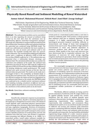
International Research Journal of Engineering and Technology (IRJET) e-ISSN: 2395-0056
Volume: 04 Issue: 12 | Dec-2017 www.irjet.net p-ISSN: 2395-0072
© 2017, IRJET | Impact Factor value: 6.171 | ISO 9001:2008 Certified Journal | Page 543
Physically Based Runoff and Sediment Modelling of Rawal Watershed
Ammar Ashraf1, Muhammad Waseem2, Nithish Mani3, Sami Ullah4, George Andiego5
1PhD Scholar, Department of Civil Engineering, Middle East Technical University, Turkey
2PhD Scholar, Faculty of agriculture and environmental sciences, Universität Rostock, Germany
3Jounior Scientist, Sahasrara Earth services & Resources Ltd, Coimbatore, India
4Lecturer, Technical Education and Vocational Training Authority (TEVTA), Lahore, Pakistan
5Water resources and environmental services department, Nairobi, Kenya
---------------------------------------------------------------------***---------------------------------------------------------------------
Abstract - The sedimentation problem can be controlled if
there is an idea regarding the amount of sediment being
carried by the river flow from the catchment area by
implementing effective watershed management strategies.
This study was undertaken to analyze sediment yield from the
Rawal Watershed. Simulation of flow and sediment yield from
the watershed was conducted using SHETRAN model. The
model was calibrated and verified for the local condition to
determine the rate of erosion and sediment yield in the
watershed. The available monthly flow data was used for
model calibration. The simulated flowyieldedgoodcalibration
results with a coefficient of efficiency (COE) of 0.98 and
Percent Bias (PBIAS) coefficient of -2. The sediment data was
generated from a relationship between discharge and
sediment load. The calculated sediment data was used for the
calibration and validation of the model. The sediment load
calibration was done for the year 2001 with the coefficient of
efficiency (COE) of 0.94 and Percent Bias (PBIAS)coefficientof
-5.8 showing satisfactory model performances. The results
obtained were quite accurate because of the fact that the
sediment data was generated. The results can be made more
meaningful if there is the availability of detailed (daily or
hourly) flow and sediment data. The land use of a catchment
was altered to analyze the impact of land use (vegetation) on
the sediment yield. Based on the results, the SHETRAN model
was confirmed to be a reliable tool for catchment sediment
yield modeling including simulation of different land uses.
Concrete efforts should be done to increase the forest area in
the catchment so that sediment yield can be decreased.
Key Words: Rawal dam, sediment modeling, SHETRAN
1. INTRODUCTION
Runoff is the catchment’s response to precipitation
resulting in stream flow. Runoff is extremely important as
the landscape is changed by its erosiveaction. Thevolumeof
runoff depends upon watershed physical characteristics
such as drainage area, elevation, slope, basin shape,landuse,
soil type, vegetation, topography, direction of orientation,
drainage network patterns etc. When it rains in catchment
area raindrop’s impact and runoff’s transport action causes
erosion. Reliable prediction of runoff quantity and rate and
sediment from land into rivers and streams is expensive,
time-consuming and difficult (Pandey et al., 2008). In a
watershed surface, runoff makes sediment available for
transport. The amount of eroded material passing througha
certain point in a watershed (outlet) within a unit time is
termed as sediment yield. Total erosion is always greater
than sediment yield due to sediment deposition during
transport. It is highly unpredictable because of the
hydrological processes temporal variability, difficulty in
measurement, and change of basin land management
practices from year to year. The problem of high sediment
concentration in rivers and sediment deposition in
reservoirs produces clear effects on land and water
resources. Water quality of the rivers and reservoirs has
been deteriorated due to suspended sediment rate. The
importance of reservoirs for water storage regarding
irrigation, hydropower generation, flood control, drinking,
and recreation purpose posesa lot of concern. It hasbecome
obligatory to consider sedimentation issues in the planning
of water resource projects.
For meaningful management of sedimentation in
rivers and reservoirs, the basic requirement is to determine
spatial soil erosion patterns and sediment yield of a
catchment. If something cannot be measured it becomes
difficult to manage. Asin sedimentation studies,theaccurate
measurement of the quantities involved is not simple. In
Pakistan, most of the small catchments in Pothowar region
have no gauging stations, especiallyforsedimentsampling.It
is also very difficult to have detailed information about the
topography, precipitationandothermetrologicalparameters
due to undulating terrain. For sustainable land and water
management reliable predictions of sediment yield is
necessary.
Worldwide, different methods are being used for
precise estimation of sediment yield. No single method can
be applied globally because each method has certain
limitations and the choice of method depends upon
catchment characteristics (ecological considerations, dam
engineering requirements, data availability, data
requirements, time availability, and economics). Many
mathematical models are in use and these models are based
on different soil erosion and sediment yield estimation
equations constituting different methods. Models are quite
helpful to simulate erosion and sediment yield processes
both spatially and temporally. During feasibilityanddetailed
engineering design studies of a water resources project,
numerical models are helpful for sediment yield analysis at
temporal and spatial scale. Numerical models can help us to
identify the sub-catchments having a major share of

sediment load into a reservoir or river. In this way, decision-
makers and planners can devise techniques to manage
sediment at specific catchment sites (sub-catchments).
Catchment management techniques are directed towards
reducing erosion at the specific problem areas. Numerical
models can also analyze and investigate climate and human-
induced changes over a required time period. As soilerosion
and sediment transport are spatially distributed processes,
so Geographic Information Systems(GIS) is consideredtobe
quite useful for soil erosion estimation. GIS provides up-to-
date, valuable spatial information on physical terrain
parameters (Chowdary et al., 2004).
The designed gross storage capacity of the Rawal
Dam was 47500 AF which has been reduced to around
31000 AF as per survey of 2009. This shows approximately
34 % reduction in storage is due to increased erosion in the
watershed areas mainly due to urbanization process. In
order to understand the soil erosion processes in the
catchment, it is better to conduct mathematical modeling of
the Rawal watershed. Physically based modeling systems
have particular advantages for the study of basin change
impacts and applications to basins with limited records.
Physically-based models are based on physical and
theoretical concepts. The modelsgivea detailed description
in time and space of the flow and transport processes that
are involved in erosion and sediment yield. The overall
objective of this study is to evaluate a physically based soil
erosion model and its accuracy to predict catchment’s
sediment yield caused by water soil erosion.
According to Smithers and Schulze (2002), the
vegetative canopy has marked effect on reducing the impact
of rainfall on the land surface as if most of the rainfall is
intercepted by a vegetative canopy, it eventually finds its
way to the surface with much less energy as compared to
direct rainfall. Variousempirical erosion models accountfor
vegetative canopy cover via taking into account different
parameters. In MUSLE, the cover management factor (C),
estimates the effect of ground cover conditions, soil
conditions, and general management practices on erosion
rates (Sadeghi et al., 2007). SHETRAN is a process-based,
spatially distributed model system for determining water
flow, contaminant migration and sediment transport(Lukey
et al., 2010). SHETRAN usesan empiricalequationtofindout
the soil erosion rate by raindrop and leaf drip impact by
taking into account the rate of detachment of soil to the
raindrop impact soil erodibility coefficient,theproportionof
ground nearly shielded by ground cover, the proportion of
ground shielded by the ground level cover and momentum
squared of raindrop and leaf drip reaching the ground per
unit time per unit area. SHETRAN solves physical based,
governing, partial differential equations for transport and
flow on a finite difference grid (Birkinshaw et al., 2010).
According to Morgan et al., (1998), the soil detachability by
raindrop impact can be uttered as the ratio of the weight of
detached soil particlesto a unit of rainfall energy. Ithasbeen
observed that if there is knowledge about the amount of
energy of a falling drop it will help in predicting the amount
of soil eroded from the ground with respect to different
standard soil textures. The rate of detachment by raindrop
impact as being proportional to the square of rainfall
intensity (Beasley et al., 1980). Pidwirny and Sidney (2008)
defined the process of entrainment as the lifting of the
particle by the erosion agents and there isa slight difference
between entrainment and detachment asitissomehowhard
to distinguish between entrainment and detachment. The
second one is mostly influenced by drag force of fluid.
Pidwirny and Sidney (2008) stated thatanentrainedparticle
will not be deposited aslong asthe velocity of the mediumis
high enough to transport the particle horizontally.Following
four different ways in which transport can occur in the
transporting medium:
 The suspension which occursin water, ice, and air is the
state in which particles are carried by the medium
without touching the surface of their origin.
 Saltation which occurs in air and water is the state in
which particle movesfrom the surface to the mediumin
rapid nonstop recurring cycles. Their returning action
to the surface generally has adequate force to cause the
entrainment of new particles.
 Traction which occurs in all media of erosion sediment
transport is the state in which there is a movement of
particles by rolling, sliding, and shuffling along the
eroded surface.
 The solution, a transport mechanism occurs only in an
aqueous environment and it generally involves
dissolving and carriage of the eroded material in water
as individual ions.
Particle weight, shape, size, medium type and surface
configuration are the main factors that decide which of the
above processes operate (Pidwirny and Sidney,2008).Julien
(1998) stated that physical processesinvolved in the spatial
and temporal variations of all the parameters describing
upland erosion from local rainstorms and bank erosion
processes exacerbate the complexityofquantifyingsediment
supply.
The sediment transported by the river has a varying
diameter. It is possible to hydraulically determine the
sediment yield in regions where the sediment transportedis
relatively coarse consisting of sand, gravel or coarser
particles (Basson and Di Silvio, 2008). Sediment load is the
quantity of sediment from a catchment passing through a
river channel’s mentioned point in a given interval of time.
Sometimestotal sediment load in a stream is usedtoexpress
sediment quantitative analysis. The sediment transport
capacity is determined as a function of the shape of the
stream cross section and hydraulic conditions. A lot of
attempts have been made to develop a relationship between
the quantity of transport material available, sediment sizes
and transport capacity.
Universal Soil Loss Equation (USLE) is one of the
empirical equations developed for computing soil losses

(Wischmeier and Smith, 1965). Further improvements have
been undertaken on the USLE method after which the
Modified Universal Soil Loss Equation, MUSLE (Williams,
1975) and Revised Universal Soil LossEquation,RUSLEwere
developed (Renard et al., 1991).
Sediment yield varies both intimeandspace.Knowledge
regarding the temporal and spatial variability extent in
sediment yields is important in resource provision for
measures to sediment control. Guyot et al. (1994)conducted
a study in the Rio Gran de, Bolivian Amazon drainage basin
(Andean river) on sediment transport. It was observed that
most of the transport occurs during three monthsoftheyear
in which water flows are high in the river. The contribution
of this period to the annual load is up to 90%. The factors
which decide whether sediment yield increase or decrease
are dependent on the site-specific conditions in accordance
with time. A number of situations shows that annual
sediment yield variability might be an indication of the
precipitation and runoff variability.
Batalla and Sala (1994) studied the temporal variability
of the suspended sediment load in a Mediterranean sandy
gravel-bed river and observed that it was causedbyseasonal
effects, extremely high sediment concentration during
individual floods and progressive exhaustion of sediment
available to be transported during storm events sequences.
The temporal variability in sediment yield is indicated by a
cumulative plot of the observed sediment load which shows
the slope in the graph of cumulative sediment discharge
against the cumulative water discharge. It wasalsoobserved
that the factors responsible for influencing the temporal
variability of sediment yield also have the ability to affect
sediment yield spatial variability to the extentwherethereis
the possibility of spatial variability in the controlling
variables within a catchment area. The temporal variation
can be annual, seasonally and even inter-annually. It,
therefore, highlights the need of long-term observeddatafor
a detailed understanding of the sediment yield temporal
variation and also to obtain sensible conclusions from
observations.
Olive et al. (1994) stated that in the Murrumbidgee
River, (New South Wales, Australia) most of the sediment
was generated from one of the localized area tributariesand
was transported through a short distance before being
deposited in the reservoir up to the main Murrumbidgee
River. This implies that the longest watercourse isn’t
essentially the major sediment source.
2. MATERIALS AND METHODS
2.1. Location, Climate, Hydrology, and Topography
Rawal Dam is situated in Pothowar plateau on
Korang River, a tributary of Soan River. Its drainage area is
264 km2 which fall in Murree, Rawalpindi, Abbottabad, and
Hazara districts. Rawal Dam Coordinates are 33°-41' N
latitude and 73°-07' E longitude. In Rawal watershed, slopes
are ranged from gentle to steep with an average of 240ftper
mile. The water in Korang River originates from rainfall and
snowmelt, with major flows during the monsoon. The
perennial flow in the river is of the order of only 3 to 6
cusecs. In the winter season, the flow is generally due to
seepage. Average annual rainfall at Rawal Dam is 46.5
inches. The main precipitation occurs during monsoon
season (July to September).
Fig 1. Location map of study area [right] and Rawal
watershed [left]
2.2 Modelling of Catchment Erosion & Sediment
Yield
2.2.1 Physically Based Models
Physically based models are based on the relationship
between physical and theoretical controlling processes.
These models simulate erosion and sediment yield both in
time and space. The models give a detailed description in
time and space of the flow and transport processes that are
involved in erosion and sediment yield. Someoftheavailable
physically based models include: Water Erosion Prediction
Project (WEPP) (Laflen et al. 1991), SHETRAN (Ewen et al.
2000), Hydrological Simulation Programme – Fortran
(HSPF) (Bicknell et al. 1997), Areal Non-point Source
Watershed Environmental ResponseSimulation(ANSWERS)
(Beasley et al., 1980), Kinematic runoff and Erosion model
(KINEROS) (Woolhiser et al., 1990), Chemicals, Runoff, and
Erosion from Agricultural Management Systems (CREAMS)
(Kinsel, 1980), and EuropeanSoilErosionModel(EUROSEM)
(Morgan et al., 1998).
2.2.2 The SHETRAN Model
Hydrological models are important tools for water
and environmental resources management (Waseem et al.,
2017). SHETRAN was developed from the Systeme
Hydrologique European (SHE) a physically based spatially
distributed (PBSD) modelling system for coupled surface
and subsurface water flow in river basins. The SHETRAN
model describes the catchment areas by using a grid and
river networks and their links. It is a 3D model having a
horizontal layer column underlying each grid square within
each soil layer in the vertical direction. The layers show the
thickness of soil and the top surface layer shows the
overland surface. Flow is routed from surface, subsurface

and up to the channel or gullies (Ewen et al., 2000).
SHETRAN model has following necessary modules: Frame
module - The main body of the model and contains input
parameters generally shared among various and allows all
modules to perform synchronized activities.
Evapotranspiration module – it calculates potential
evapotranspiration from the soil, vegetation and water
surfaces, evaporation from bare soil, wetted canopies, free
water surfaces, dry channels and also computes
transpiration by plants. Overland/channel module – it
computes the surface water depth on theground,inchannels
and calculates surface water flow across the ground surface
and in channels. Variably saturated subsurface module – it
simulates three-dimensional water flow in the subsurface
soil scheme including seepage (Ewen et al, 2000).
2.3 Description of the Data
2.3.1 Metrological data
Precipitation and evaporation data was collected
from Satrameel Meteorological station, situated in Rawal
watershed. The data was available only on daily bases. The
rainfall data was of good quality, while evaporationdatawas
missing for a lot of years. Discharge data of Korang riverwas
also available on monthly bases. At dam site, there was no
mechanism for systematic measurement of discharge data
on daily bases and there was a lot of ambiguities in the data.
2.3.2 Sediment Data
At the dam site, there was no mechanism for
systematic measurement of sedimentdata.So,sedimentdata
was not available for the dam site. The only type of sediment
data available was in the form of Hydrographic surveys
(Sedimentation surveys). In ordertogeneratesedimentdata,
the Rawal lake survey range lineswere digitized for theyear
1996 and 2000 using ArcGIS software. After digitizing the
maps, the surface volume wascompared atdifferentlevelsto
have the volume of deposited sediment in last four years.
2.4 Generation of Digital Maps of Hydrographic
Survey
For digital map generation, the range linessurveyof
years 1996 and 2000 were digitized by ARC GIS. After
developing digital maps for years 1996 and 2000, the
volume at different elevations were calculated using 3D
Analyst Tool > Surface Analysis > Area and Volume
command. Then volume difference at same elevations was
calculated for years 1996 and 2000 that gives change in
volume of the reservoir with the passage of time.
2.5 Data Processing and Analysis
2.5.1 Rainfall-Runoff Analysis
For the year 2001, 2002, 2004 and 2005, rainfall
and runoff data were analyzed by drawing it on same graph
with inflow (Runoff) and rainfall data on primary and
secondary Y-axis respectively and time in months on X-axis.
For the year 2001, the graph shows a good relationship
between the inflow and the rainfall as both rainfall and
inflow peaks were observed in the same month.
1 2 3 4 5 6 7 8 9 10 11 12
0
200
400
600
800
1000
1200
1400
0
20000
40000
60000
80000
100000
120000
140000
160000
0 2 4 6 8 10 12
Time (Months)
Rainfall(mm)
Inflow(AF)
Time (Months)
Rainfall
Dischage 2001
Fig 2. Rainfall-runoff comparison 2001
For the year 2002, the graph (Fig. 3) also shows a
good relation between the inflow and the rainfall as in the
8th month the peak runoff and rainfall was observed.
1 2 3 4 5 6 7 8 9 10 11 12
0
100
200
300
400
500
600
700
800
900
10000
10000
20000
30000
40000
50000
60000
70000
80000
90000
100000
0 2 4 6 8 10 12
Time (Months)
Rainfall(mm)
Inflow(AF)
Time (Months)
Rain
Discharge 2002
Similarly, the graph (Fig 4) also shows a good
relation between the inflow and the rainfall for the year
2004. Asboth rainfall and inflow peakswere observedinthe
same month i.e. August.
1 2 3 4 5 6 7 8 9 10 11 12
0
100
200
300
400
500
600
7000
5000
10000
15000
20000
25000
30000
35000
0 2 4 6 8 10 12
Time (Months)
Rainfall(mm)0
Inflow(AF)
Time (Month)
Rainfall
Dischage 2004

For the year 2005, the graph (Fig. 5) showed that in
comparison to three rainfall peaks there are only two runoff
peaks. It indicates that there is a problem with discharge
data for this year.
1 2 3 4 5 6 7 8 9 10 11 12
0
100
200
300
400
500
600
700
800
900
10000
5000
10000
15000
20000
25000
0 2 4 6 8 10 12
Time (Months)
Rainfall(mm)
Inflow(AF)
Time (Months)
Rain
Discharge 2005
2.5.2 Rainfall-Runoff Ratio
Rainfall-runoff ratiosfor theyears2001,2002,2004
and 2005, were calculated by adding up the monthly rainfall
volume and then runoff volume was converted into depth
(mm) by dividing it with the catchment area.
2.6 Topographic Analysis for DEM Extraction
Rawal watershed DEM was extracted by using Arc
hydro tools in a specified manner in ArcGIS software. The
Rawal DEM obtained is shown below.
Fig 6. Rawal Watershed DEM
2.7 Results Analysis
Model output was in the hourly form. As the
available runoff and sediment data were in form of monthly
data, the hourly data was summed up into monthly data by
using excel. The results were then compared to have a good
simulation. After a good simulation was achieved then the
model output was evaluated through coefficient as COE and
PBIAS.
The coefficient of efficiency (COE) or Nash-Sutcliffe
efficiency (NSE) is the statistical criterion for evaluation of
goodness of fit between observed and calculated values.
Nash-Sutcliffe efficiencies range from Infinity to 1.
Essentially, the closer to 1, the more accurate the model is,
equal to 1 corresponds to a perfect match of modeled to the
observed data, equal to 0 indicates that the model
predictions are as accurate asthe mean of the observed data
and in range of Infinity < NSE < 0, indicatesthattheobserved
mean is a better predictor than the model. The coefficient of
model efficiency (COE) wascalculated(Nash-Sutcliffe,1970)
as:
Where
Si= Simulated value
Oi= observed value
= Mean Observed
Percent bias (PBIAS) measures the average tendency of
the simulated values to be larger or smaller than their
observed ones. The optimal value of PBIAS is 0.0, with low-
magnitude values indicating accurate model simulation.
Positive values indicate overestimation bias, whereas
negative values indicate model underestimation bias.
Percent bias (PBIAS) was calculated (Yapo et al. 1996) as.
Where
Si= Simulated value
Oi= observed value
3. RESULTS AND DISCUSSION
3.1 Model setup
The total catchment area is 264 km2, which was
represented by 264 grid squares of 1km by 1km each. The
elevations ranged from around 2258 masl (highest point)to
393 masl (lowest point). The dominant soil type within the
catchment is clay-loam. The main type of vegetationisforest.
Major land usesare forest and urbanization. The canopyand
leaf parameterssuch ascanopy drainage,canopystorageand
vegetation cover indiceswere basedonstandardparameters
specified in SHETRAN Version 4 User Guide (2008) for
variousstandard vegetation types. TheManning’sroughness
coefficient for channels was taken as 0.035 (Strickler
resistance coefficient as 29).
3.2 Flow calibration
Upon setting up the appropriate hydrological,
meteorological, spatial data, the model was calibrated
against observed flow for the year 2001.Themostsignificant
Legend
Rawal DEM
Value
High : 2004
Low : 523

hydrological and flow calibration parameters that were
slightly adjusted included the following: Stickler’s overland
flow coefficient, vegetation parameters (canopy storage
capacity (mm), leaf area index, saturated conductivity and
unsaturated conductivity and soil depths. Daily rainfall and
evaporation data were used with the data time step of 24
hours. The output from the model washourly flow data. The
hourly data was then converted into monthly data for
comparison with the observed flow. The accuracy of the
calibration was verified by comparing the simulated flows
with observed flows as shown in fig 7. The R2 was found to
be 0.82. For calibration results COE and PBIAS coefficients
were calculated to be 0.98 and -2 respectively, which
showed satisfactory model performance.
0
5000
10000
15000
20000
25000
30000
35000
0 2 4 6 8 10 12
Discharge(cumecs)
Time (Month)
Observed
Simulated
Fig 7. Flow Calibration for year 2001
As the results were obtained a comparison of
observed and simulated values were made to obtain a
correlation between them. Observed data was plotted on X-
axis while the simulated data was plotted on Y-axis. After
plotting the data, best fit trend line was selectedanditsvalue
of R2 was noted. For year 2001 it was observed that there
was high flow in only one month while in rest of the months
the flow was low. This is the reason that most of the values
on graph gather at the bottom left of the graph and only one
value is seen away from this mob of values.
R²= 0.82
0
5000
10000
15000
20000
25000
30000
0 4000 8000 12000 16000 20000 24000 28000 32000
Simulated(Cumecs)
Observed (cumecs)
Fig 8. Comparison of observed and simulated discharge for
year 2001
3.3 Flow validation
After calibrating the model, it wasvalidatedforyear
data 2002, 2004 and 2005. As mentioned earlier there was
problem with data as the observed data was of poor quality.
When rainfall-runoff analysis was done for year 2003 it was
observed that the months having high rainfall don’t have
high flows and vice versa. Similarly, for 2003 the validation
comparison of observed and simulated data was very poor.
For year 2002 the model validation results were quite good.
The R2 value of best fit trend line was found to be 0.83. The
observed and simulated data values were used for
calculating COE and PBIAS coefficients which turned out to
be 0.97 and -8.
Fig 9. Flow validation for year 2002
The simulated results for year 2002werecompared
with the observed one to determine the R2 value which was
observed to be 0.83. Only two points can be seen to have
maximum values while for rest of the months the values are
mobbed near the point of origin.
R²= 0.83
0
3000
6000
9000
12000
15000
0 3000 6000 9000 12000 15000
Simulated(cumecs)
Observed (cumecs)
Fig 10. Comparison of observed and simulated discharge
for year 2002
For year 2004 the model results were also quite
good. The model calculated the peaks in same months in
which the peaks were observed. The R2 value was found to
be 0.92.

Fig 11. Flow validation for the year 2004
In the comparison graph for the year 2004, seven
values mobbed around the point of origin while the rest
scattered around the trend line. The coefficients values for
COE and PBIAS were calculated to be 0.93 and 7.
R² = 0.92
0
1000
2000
3000
4000
5000
6000
7000
8000
9000
0 1000 2000 3000 4000 5000 6000 7000
Simulted(cumecs)
Observed (Cumecs)
for the year 2004
For the year 2005 the simulated value showed one
peak while the observed data showed two peaks. But the
annual runoff volume wasquite close to theannualobserved
data.
Fig 13. Flow validation for the year 2005
The comparison graph for the year 2005 showed
six-month values mobbed around the origin while the rest
scattered around the trend line. The R2 value was observed
to be 0.83. The values for COE and PBIAS coefficients were
calculated to be 0.86 and 14.
R² = 0.83
0
2000
4000
6000
8000
10000
12000
14000
0 1000 2000 3000 4000 5000 6000
Simulated(Cumecs)
Observed (Cumecs)
for the year 2005
After validating the model, the input files for
SHETRAN standard are written and the output shegarph file
is also generated which is viewed using HDF software. In
shegarph file, catchment map shows elevation and river
network pattern in the catchment area.
Fig 15. SHETRAN generated Rawal catchment palette
showing elevation and rivers as links
3.4 Sediment Calibration and Validation
After getting a reasonable flow simulation the
SHETRAN Standard input files were written using write
Shetran input filestool. The sediment file is notgeneratedby
the above command. The sediment filewasmanuallywritten
as it has to be manually generated for each catchment
according to the catchment characteristics. The check
visualization plan file was also adjusted in order to achieve
the required results. Sediment calibration was done for the
year 2001 by comparing the model results from the results
of hydrographic survey digitization. After obtaining a good
calibration the model was validated for years 2002, 2004
and 2005. The model output was on hourly bases; it was
converted into monthly bases by usingexcel.Theparameters
used in sediment file are given below.

Table 1. Soil parameters used in Sediment file
Parameter Average/range
Overland flow soil erodibility 1.3x10-12 to 7x10-
11*kgm-2s-1
Raindrop and drip soil
erodibility
0.1j-1
Threshold depth of loose soil
over which erosion is zero
0.05m
Channel bank erodibility
coefficient
1x10-11 kgm-2s-1
* rate of detachment of soil per unit area.
3.4.1 Sediment Load Calibration
SHETRAN Standardmodelsedimentloadcalibration
was done for the year 2001. The model parameters were
varied such that the model output is close to the calculated
sediment data. The model output wason hourlybasesit was
converted into monthly bases. The results are shown in fig
16 The results were then used to calculate the COE and
PBIAS coefficients which were 0.94 and -5.8 respectively.
The results showed that model performance was
satisfactory.
0
2000
4000
6000
8000
10000
12000
0 2 4 6 8 10 12
Sedimentload(tons)
Time (Months)
Observed
Simulated
Fig 16. Sediment load Calibration 2001
The cumulative graph was also drawn as shown in
fig 17. The total simulated sediment load was 17816 tons
and the observed load was 19976 tons.
0
5000
10000
15000
20000
25000
0 2 4 6 8 10 12
Sedimentload(TONS)
Time (Months)
Observed
Simulated
Fig 17. Observed and Simulated sediment load cumulative
graph 2001.
3.4.2 Sediment Load Validation
The model was validated for the year 2002. The
parameters used in calibration were kept same for
calibration purpose. The model output washourly sediment
discharge. The model output was compared with the
sediment data calculated by using the developedcorrelation.
The comparison between model-simulated and calculated
sediment load is shown in Fig. 18. It can be seen that the
simulated and calculated curves match well except for few
months. The correlation coefficient was 0.97 while the COE
and PBIAS were 0.96 and -6 respectively, which showedthat
model performance was satisfactory.
0
2000
4000
6000
8000
10000
12000
0 2 4 6 8 10 12
Sedimentload(tons)
Time (Months)
Observed
Simulated
Fig 18. Sediment Validation 2002
and the calculated load was 12767 tons.
0
2000
4000
6000
8000
10000
12000
14000
0 2 4 6 8 10 12
Sedimentload(TONS)
Time (Months)
Observed
simulated
graph 2002
After model validation, it was applied to the year
2004. The results depicted that model overestimates the
calculated results. PBIAS coefficient with a value of 12 also
shows that model overestimates the results. The COE value
was calculated to be 0.98 which suggested that model
performance was satisfactory.

0
500
1000
1500
2000
2500
3000
3500
4000
4500
0 2 4 6 8 10 12
Sedimentload(Tons)
Time (Months)
Observed
Simulated
Fig 20. Model Application 2004
fig 21. The total simulated sediment load was 7738 tons and
the calculated load was6889 tons, which showedthatmodel
overestimates the results.
0
1000
2000
3000
4000
5000
6000
7000
8000
9000
0 2 4 6 8 10 12
SedimentLoad(Tons)
Time (Months)
Observed
simulated
graph 2004
The model was also applied to the year 2005. The
results obtained showed that the model somewhat
overestimates the results. This isbecause of the poorquality
of data. The COE and PBIAS coefficientswerecalculatedtobe
0.96 and 16 respectively.
0
1000
2000
3000
4000
5000
6000
7000
0 2 4 6 8 10 12
Sedimentload(Tons)
Time (Months)
Observed
Simulated
Fig 22. Model Application 2005
and observed load was 8639 tons which showed that model
overestimates the results.
0
2000
4000
6000
8000
10000
12000
0 2 4 6 8 10 12
Sedimentload(Tons)
Time(Months)
Observed
Simulated
graph 2005
3.5 Land Use Sensitivity Analysis
Sensitivity analysis for land use parameters was
done by changing the vegetation types. The major type of
land use in the catchment is forest i.e. 48%. The sensitivityof
sediment yields to increase or decrease in forest area was
checked. The results were found reasonable, as an increase
in forest area showed a decrease in sediment yield while a
decrease in forest area resulted in an increase in sediment
yield. The decrease in sediment yield was calculated to be
from 75 tons/Km2 to 62 tons/Km2. It was observed that for
10 % increase in forest area sediment yield decreased up to
17%. On the other side, 10 %decrease in forestarearesulted
in 12% increase in sediment yield i.e. from 75 tons/Km2 to
84 tons/Km2. Further investigation should be donebasedon
results to find the best effective watershed management
technique for controlling erosion.
Table 2. Land use sensitivity of sediment yield in terms of
forest area
Status of
Forest Area
Forest area
(%)
Sediment yield
(tons/Km2)
Present 48 75
Increased 58 62
Decreased 38 84
4 Conclusion
Following conclusions have been drawn from the
results of this study;
 The flow simulation yielded satisfactory results. Peaks
flows were observed generally during the monsoon
period, while in the rest of the months the flows were
quite low as compared to peak flow.
 For the year 2005 rainfall runoff comparison graph
showed the observed data was of poor quality, as the
months in which peak rainfall was recorded did not
have peak runoff and vice versa.

 The sediment modelling calibration was done against
the sediment data which was actually generated from
the relation to runoff and sediment.
 The sediment modelling results were quite accurate.
This was due to the fact that the calculated sediment
data was used for calibration and validation purpose as
there was no observed sediment data.
 The mean annual sediment load was calculated to be 45
tons/Km2.
 The model sensitiveness to land use change was also
checked and it was concluded that the model responds
reasonably to catchment land use changes.
 In the reservoir on the right side of dam, a deposition
pattern was observed while on the left side therewasno
deposition pattern.
REFERENCES
1. Horng, Y.T., Soo, P.C., Shen, B.J., Hung, Y.L., Lo, K.Y., Su,
H.P., Wei, J.R., Hsieh, S.C., Hsueh, P.R. and Lai, H.C.,
(2006). Development of an improved PCR-ICT hybrid
assay for direct detection of Legionellae and Legionella
pneumophila from cooling tower water specimens
Water research, 40 (11). 2221-2229.
2. Basson, G.R., and Di Silvio, G. (2008). Erosion and
sediment dynamics from catchment to coast. UNESCO.
International Hydrological Programme, Technical
Documents in Hydrology, No 82.
3. Batalla, R.J., and Sala, M. (1994). Temporal variability
of suspended sediment transport in Mediterranean
sandy gravel bed river. IAHS Publication 224.
4. Beasley, D.B., Higgins, L.F., and Monk, E.J. (1980).
ANSWERS. A model for watershed planning,Trans.,Am.
Soc. Agric. Eng., 23: pp. 938-944.
5. Bicknell, B.R., Imhoff, J.C., Kittle, J.L., Donigian,A.S.and
Johanson, R.C. (1997). Hydrological Simulation
Program-Fortran: User's manual for version 11: U.S.
Environmental Protection Agency, National Exposure
Research Laboratory, Athens, Ga., EPA/600/R-97/080.
6. Birkinshaw, S. J., James, P., & Ewen, J. (2010).
Graphical user interface for rapid set-up of SHETRAN
physically-basedrivercatchmentmodel. Environmental
Modelling & Software, 25(4), 609-610.
7. Chowdary, V.M., Yatindranath, Y., Kar, S., Adiga, S.,
2004. Modeling of non-point source pollution in
watershed using remote sensingand GIS. J. Indian Soc.
Remote Sensing 32 (1), 59–73.
8. Ewen, J., Parkin, G., and O’Connell, P.E. (2000).
SHETRAN: Distributed river basin flow and transport
modelling system. Proceedingsof the American Society
of Civil Engineers, Journal of Hydrologic Engineering 5,
pp. 250-258.
9. Ewen, J. Parkin, G and O’Connell “SHETRAN:
DISTRIBUTED RIVER BASIN FLOW AND TRANSPORT
MODELLING SYSTEM” Journal of Hydrologic
Engineering, Vol. 5, No. 3, July, 2000.QASCE,ISSN1084-
0699/00/0003-0250–0258
10. Guyot, J.L., Bourges, J., and Cortex, J. (1994). Sediment
transport in Rio Grande, an Andean riveroftheBolivian
Amazon drainage basin. Variability in stream erosion
and sediment transport, IAHS Publication 224,pp.223-
231.
11. Kinsel, W.G. (1980). CREAMS: A field scale model for
Chemicals, Runoff, and Erosion, in Agricultural
Management Systems. U.S. Department of Agriculture,
Conservation Report no. 26, pp. 640.
12. Lukey, B. T., Sheffield, J., Bathurst, J. C., Hiley, R. A., &
Mathys, N. (2000). Test of the SHETRAN technologyfor
modelling the impact of reforestation on badlands
runoff and sediment yield at Draix, France. Journal of
Hydrology, 235(1), 44-62.
13. Morgan, R.P.C., Quinton, J.N., Smith, R.E., Govers, G.,
Poesen, J.W.A., Auerswald, K., Chisci, G., Torri, D.,
Styczen, M.E., and Folly, A.J.V. (1998). The European
Soil Erosion Model (EUROSEM): Documentation and
user guide.
14. Olive, L.J., Olley, J. M., Murray, A.S. & Wallbrink, P.J.
(1994) Spatial variation in suspended sediment
transport in the Murrumbidgee River, New south
Walse, Australia. In variability in stream erosion and
sediment transport, 241-249. IAHS Publ. no. 224.
15. Pandey, A., Chowdary, V. M., Mal, B. C., & Billib, M.
(2008). Runoff and sediment yield modeling from a
small agricultural watershed in India using the WEPP
model. Journal of Hydrology, 348(3), 305-319.
16. Pidwirny, M., Sidney D. (2008). Soil erosion and
deposition. Encyclopaedia of Earth (Washington, D.C.:
Environmental Information Coalition, NationalCouncil
for 102 Science and the Environment
<http://www.eoearth.org/article/Soil_erosion_and_dep
osition>http://www.eoearth.org/article/Soil_erosion_a
nd_deposition.
17. Renard, K.G., FOSTER, G.R., WEESIES, G.A., and
PORTER, J.P. (1991). RUSLE: Revised Universal Soil
LossEquation. J. Soil and Water Cons., 46(1), pp. 30-33.
18. Sadeghi, S.H., Mizuyama, T., and Vangah, B.G. (2007).
Conformity of MUSLE estimates and erosion plot data
for storm-wise sediment yield estimation. Terr. Atmos.
Ocean. Sci., Vol. 18, No. 1, pp. 117-128.

19. Smithers, J., Schulze, R. (2002). ACRU
Agrohydrological Modelling System User Manual
Version 3.0.0.
20. Waseem, M., Mani, N., Andiego, G., & Usman, M.
(2017). A Review of Criteria of Fit for Hydrological
Models.
21. Williams, J.R. (1975). Sediment yield prediction with
universal equation using runoff energy factor, In:
Present and Prospective Technology for Predicting
Sediment Yields and Sources. USDAARS, 40, pp. 244-
252.
22. Wischmeier, W.H. and D.D. Smith. 1965. Predicting
rainfall-erosion losses from cropland east of the Rocky
Mountains – Guide for selection of practicesforsoiland
water conservation. U.S. Dept. Of Agric., Agr. Handbook
No. 282.
23. Woolhiser, D.A., R.E. Smith and D.C. Goodrich.1990.
KINEROS, A Kinetic Runoff and Erosion Model:
documentation and user manual. USDA- Agricultural
Research services, ARS-77, pp 130.
24. Yapo P. O., Gupta H. V., Sorooshian S, (1996).
Automatic calibration of conceptual rainfall-runoff
models: sensitivity to calibration data. Journal of
Hydrology. V181 i1-4. 23-48.

Physically Based Runoff and Sediment Modelling of Rawal Watershed

Empfohlen

Empfohlen

Weitere ähnliche Inhalte

Was ist angesagt?

Was ist angesagt? (18)

Ähnlich wie Physically Based Runoff and Sediment Modelling of Rawal Watershed

Ähnlich wie Physically Based Runoff and Sediment Modelling of Rawal Watershed (20)

Mehr von IRJET Journal

Mehr von IRJET Journal (20)

Kürzlich hochgeladen

Kürzlich hochgeladen (20)

Physically Based Runoff and Sediment Modelling of Rawal Watershed