1. Big Matrix Completion With Soft-impute
Singular Value Decomposition
Xiyuan Sun, 1
Hengfang Wang1
,Yifan Wang1
, Xiaofei Zhang1
1 INTRODUCTION
Matrix Completion (MC) is the problem of recovering a matrix from only a small sample of
its entries. The goal of matrix completion is to impute the missing entries of a large matrix
based on the information given by the limited entries. (Wong, 2015) The theory behind MC
is that the matrix is low-rank then we can exactly recover the original matrix.
In this final project, we look into one of its most popular application to movie recommend
system. In such context, the low rank means that users can be divided into groups with
similar tastes. With this assumption, we can devise a convex optimization problem to recover
the original matrix A with missing entries. Our objective is to minimize rank(A) subject to
its projection on observation subset, where the P-omega operator sets values values outside
omega (omega is the set of observed entries of A) to zero and keeps those in omega. M
is our partially observed matrix(the ratings). The constraint ensures that the observed
values are preserved in A. Unfortunately minimizing the rank is an NP-hard problem. We
replace the closest convex envelope which is the nuclear norm. Our actual objective is
minimizing nuclear norm of A with weights subject on P-omega. Solving this nuclear norm
minimization problem will recover our user ratings, which we can use as recommendations.
We are interested in a specific of the algorithm (Soft-impute SVD) to solve the convex
optimization problem.(Tiemey, 2014)
We used the data collected by the GroupLens Research Project at the University of
Minnesota. The data set consists of 100,000 ratings (1-5) from 943 users on 1682 movies.
Each user has rated at least 20 movies. Each row of the matrix (userid) consists of ratings
1
Department of Statistics, Iowa State University

2. from a particular customer, while each column (itemid) records the ratings for a particular
movie. Demographical information and movie information were also included in the data
zip file. In the ml-100k dataset, the missing rate is 1486126/1586126 (93.7%). In another
word, only 6.3% of the ratings are observed. Without any prior knowledge, a reasonable full
recovery of the matrix is virtually impossible. To overcome this issue, it’s common to assume
that the matrix is low rank, assuming that the users’ ratings are based on a relatively small
number of factors. Various convex relaxations and related optimization algorithms have been
proposed in many applications. (Wong, 2015) Here we adopted the soft-impute singular value
decomposition algorithm and nuclear norm approximation to impute the target matrix since
the theoretical properties of matrix completion using nuclear norm minimization have been
well studied. (Wong, 2015)
In the following part, we utilized five methods to do the svd in r. First method just used
the built-in svd function. Second used the propock.svd from the svd package. Third used
the irlba package. Fourth used the RcppArmadillo library. Fifth used the fast.svd in corpcor
package. First we tried all of the methods with our generated small matrix of different
sizes and different missing rate. Then we took the big matrix from the movie dataset to be
our input of those algorithms. We compared the computational time and training errors of
different methods in all the scenarios. After comparing them in the large-scale data context,
we conclude that fast.svd is the most efficient one when we take both time and test error
into consideration. Even though irlba tends to have some advantages in speed, its accuracy
is not as competitive as fast.svd. The performance of these methods in small-scale scope is
different from that in the large-sclae context. If you would like to know more details about
our project, please check our source code and the tables in the result section.
2 Experimental Design with Different Methods
In the numerical linear algebra literature, There are very efficient direct matrix factorization
methods for calculating the SVD of a matrices of moderate size (at most a few thousands).
2

3. When the matrix is sparse, larger problem can be solved but the computational cost depends
heavily upon the sparsity structure of the matrix. In general, one has to resort to indirect
iterative methods for calculating the leading singular vectors/values of a matrix.(Mazumder
et. al 2010)
We will use the PROPACK algorithm because of its low storage requirements, effective
flop count and its well documented MATLAB version. The algorithm for calculating the
truncated SVD for a matrix W. It becomes efficient if multiplication operations Wb1 and
W b2 (with b1 ∈ Rn
, b2 ∈ Rm
) can be done with minimal cost.(Mazumder et. al 2010)
Algorithm SOFT-IMPUTE requires repeated computation of a truncated SVD for a
matrix W. The cost of computing the truncated SVD will dependent upon the cost in the
operations Wb1 and W b2. The computational order of SOFT-IMPUTE and that of SVT is
the same. The computational cost of evaluating the truncated SVD (with rank r) is linear in
matrix dimensions. This justifies the large-scale computational feasibility of our algorithm.
In our small-scale experiments, we want to try some matrices with different sparsity
structure Numerical Experiments and Comparisons. We use the underlying model Zm×n =
Um×r ∗ Vr×n, where U and V are random matrices with standard normal Gaussian entries Ω
is uniformly random over the indices of the matrix with p% of missing entries these are the
models under which the coherence conditions hold true for the matrix completion problem
to be meaningful
The Training Error can be defined as
||Zold−Znew||2
F
||Zold||2
F
over the Ω set The fraction of the error
explained on the observed entries by the estimate relative to a zero estimate In different
scenarios, we change the dimension of the matrix (m,n) and missing rate p.
For SOFT-IMPUTE we consider a equi-spaced grid of 20 lambda in the range of
[λmin, λmax]. λmin is a full-rank solution of SOFT-IMPUTE. λmax is the zero solution. Here
we just simplified it to be from 1 to 20. (estimatedU , estimatedV ) were solved for over the
grid of λ values.
SOFT-IMPUTE was run untill a tolerance of 10−4
was achieved For every algorithm,
3

4. total time indicates the time required for evaluating solutions over the entire grid of lambda
values.
In these examples, we used SVD factorization with four different methods for the SVD
computation To summarize, we study the following methods:
1. SOFT-IMPUTE with built-in svd function
2. SOFT-IMPUTE with the svd function given in the svd package (propack)
3. SOFT-IMPUTE with the irlba
4. SOFT-IMPUTE with the RcppArmadillo
5. SOFT-IMPUTE with the corpcor
In all these examples, We observe that SOFT-IMPUTE performs very favorably in terms
of total times.We need to generate a table based on our experiments.
PΩ(X) + P⊥
Ω (Zk
λ) can be rewritten as PΩ(X) − P⊥
Ω (Zk
λ) + Zk
λ = Sparse + Low Rank
Report our findings on such simulation examples. Our Inputs are:
• Dimension: (m,n);
• Missing rate: |Ω|
mn
;
• λgrid (20 lambdas).
Output:
• training error
• time
The Training Error can be defined as
||Zold−Znew||2
F
||Zold||2
F
over the Ω set maybe we also need to
save the recovered solution and keep track of their ranks total time required to perform the
SVD computations over all iterations of the algorithm
4

5. 2.1 Algorithms in different methods
2.1.1 R internal svd function
The main functions used are the LAPACK routines DGESDD and ZGESDD. LAPACK is
from http://www.netlib.org/lapack and its guide is listed in the references.
2.1.2 svd package
We use propack.svd function in svd package. The other two functions in that package,
trlan.svd and ztrlan.svd, will not return V matrix, so for convenience, we will not use
them.
The function provides an interface to a state-of-art implementations of truncated SVD
— PROPACK, which does this via the implicitly restarted Lanczos bidiagonalization with
partial reorthogonalization.
Currently, the computation of small singular values is not very robust, because con-
vergence of the methods discussed in this report is likely to be slow or, in some cases,
unattainable. In order to be more likely to get convergence to small singular values, it would
be necessary to incorporate techniques such as harmonic or refined Ritz projections.
2.1.3 RcppArmadillo
We use svd function in RcppArmadillo. The method argument is optional; method is either
”dc” or ”std”
• ”dc” indicates divide-and-conquer method (default setting)
• ”std” indicates standard method
the divide-and-conquer method provides slightly different results than the standard method,
but is considerably faster for large matrices.
5

6. 2.1.4 irlba package
We use irlba function in irlba package. The augmented implicitly restarted Lanczos bi-
diagonalization (IRLBA) algorithm finds a few approximate largest singular values and cor-
responding singular vectors of a sparse or dense matrix using a method of Baglama and
Reichel. It is a fast and memory-efficient way to compute a partial SVD.
2.1.5 Fast svd
We use fast.svd in corpcor package. The main difference to the native version svd is that
fast.svd is substantially faster for ”fat” (small n, large p) and ”thin” (large n, small p)
matrices. In this case the decomposition of M can be greatly sped up by first computing
the SVD of either MM (fat matrices) or M M (thin matrices), rather than that of M. A
second difference to svd is that fast.svd only returns the positive singular values (thus the
dimension of D always equals the rank of M). Note that the singular vectors computed by
fast.svd may differ in sign from those computed by svd.
2.2 Comparisons Results
2.2.1 Change in dimensions (keep the missing rate the same)
The computation time for the five methods illustrated above under the same missing rate
0.6 with different dimensions is presented as follows:
Dimension R Internal propack.svd irlba RcppArmadillo Fast svd
(10,10) 0.01 0.02 0.20 0.28 0.30
(100,100) 0.47 0.71 0.42 0.58 0.57
(200,100) 0.90 0.93 0.45 1.18 0.92
(500,500) 43.23 59.42 1.45 40.68 35.48
(800,800) 3.66 4.63 3.87 2.79 135.44
Table 1: Computation time under same missing rate 0.6 with different dimensions
6

7. The training error for the he five methods illustrated above under the same missing rate
0.6 with different dimensions is presented as follows:
Dimension R Internal propack.svd irlba RcppArmadillo Fast svd
(10,10) 0.26 0.26 0.23 0.51 0.70
(100,100) 0.32 0.32 3.85 0.32 0.36
(200,100) 0.29 0.29 3.39 0.42 0.35
(500,500) 0.65 0.65 2.77 1.05 0.96
(800,800) 0.89 0.89 2.87 1.32 1.23
Table 2: Training error under same missing rate 0.6 with different dimensions
The two tables above can be presented as follows:
7

8. When the matrix is very small in size (10x10), the most efficient algorithm is given by
the build-in svd function. The propack.svd from the svd package seems to be the same as
the build-in svd in terms of the performance (the same time, the same error). But when
we adopt the irlba package, the time jumps up abruptly while the training error decreases a
little bit. The time keeps going up at a lower rate for armadillo svd and fast.svd, while their
training error steadily pumped up.
When the matrix’s dimension goes up to (100,100), the performance of buid-in svd func-
tion and the fast.svd are the top efficient ones. Irlba package gives us a large error with
comparatively shorter time consumption. (200,100) has a similar outcome.
When we come up with the largest one (800x800) in our experiments, the first four
methods keep the performance at the same level. But the time for fast.svd pumps up
magically.
Considering the randomness of running the experiment only for one time, we run 50 times
for same missing rate 0.6 with different dimensions, the median of the time consuming is
presented as follows:
Dimension R Internal propack.svd irlba RcppArmadillo Fast svd
(10,10) 0.02 0.03 0.34 0.02 0.02
(20,20) 0.04 * 0.7 0.04 0.04
(50,50) 0.29 0.47 2.76 0.27 0.26
(100,100) 1.4 * 9.99 1.35 1.16
8

9. Note that this experiment did not run on the same machine as the previous experiments
with one run.
The sign ∗ means that the program broke out due to some program failure(application of
propack), indicating that propack approach is not reliable. As we can see, as the dimensions
of the matrices increase, the time for each method is increasing correspondingly. When
compared among different method, ’Fast svd’ is the best in speed, while irlba is with the
slowest one.
2.2.2 Change in missing rate (keep the dimension the same)
The computation time for the five methods illustrated above under the same dimension
100 × 100 with different missing rates is presented as follows:
Missing Rate R Internal propack.svd irlba RcppArmadillo Fast svd
0.4 0.50 0.60 0.34 0.54 0.53
0.5 0.42 0.66 0.41 0.41 0.53
0.6 0.48 0.69 0.42 0.57 0.54
0.9 0.63 0.93 0.49 0.80 0.74
Table 3: Computation time under same dimension 100 × 100 with different missing rates
The training error for the five methods illustrated above under the same dimension 100×
100 with different missing rates is presented as follows:
Missing Rate R Internal propack.svd irlba RcppArmadillo Fast svd
0.4 0.18 0.18 0.72 0.23 0.21
0.5 0.23 0.23 1.88 0.31 0.27
0.6 0.32 0.32 3.33 0.44 0.36
0.9 0.76 0.76 10.35 1.58 0.90
Table 4: Training error under same dimension 100 × 100 with different missing rates
Error distributions among all the methods with different missing rate are similar, with
9

10. a peak at the third method. The change trend for the time is also the same among all the
missing rates. In terms of the absolute value comparison, as the missing rate increases, both
the time and the training error tend to increase at the same time.
Considering the randomness of running the experiment only for one time, we run 50
times for the same dimension 100 × 100 with different missing rates, the median of the time
consuming is presented as follows:
Missing Rate R Internal propack.svd irlba RcppArmadillo Fast svd
0.4 1.02 1.54 7.13 0.98 0.83
0.5 1.14 1.73 8.19 1.09 0.93
0.6 1.40 * 9.98 1.35 1.15
0.9 1.17 1.77 8.21 1.11 0.95
Note that this experiment did not run on the same machine as the previous experiments
with one run.
The sign ∗ means that the program broke out due to some program failure(application
of propack), indicating that propack approach is not reliable. As we can see, as the missing
rate goes from 0.4 to 0.6, the time for each method is increasing correspondingly. However,
when it comes to missing rate with 0.9, due to sparsity of the matrix, the time goes down.
When compared among different methods, ’Fast svd’ is the fastest, while irlba is the slowest
one.
2.3 Bonus Part Algorithm
The method we use here is called FRSVD. We use random numbers to sample from matrix
A through adaptive rank prediction heuristicly. The dimension of the matrix shrinks down
to be used in SVD, which contributes a lot in the speed improvement. We also utilize power
iteration in order to make the spectrum difference larger. The efficiency of this method may
be degraded by an excessively high sampling rate.
10

11. 2.4 C Programme
We write C program for Soft-Impute with 2 versions: one is the standard one(2.1) and the
other is an accelerated version(4(bonus)). It works well for both versions. Please refer to
the C program in the src folder for more details.
3 Real Data Analysis
3.1 Snap of the original data
We will apply Soft-Impute to the MovieLens datasets obtained via
http://grouplens.org/datasets/movielens/. MovieLens data sets were collected by the Grou-
pLens Research Project at the University of Minnesota. We use the 100k dataset which
consists of 100,000 ratings (1-5) from 943 users on 1682 movies. In the data set, each user
has rated at least 20 movies. So the missing rate of this data set is 93.7%.
3.2 Split method and the measurement to try in the assessment
step
We randomly split the data set into three subsets: training set, validation set and test set with
70%, 15%and 15% of the original dataset respectively. First apply the Soft-Impute algorithm
to the training dataset with a set of λ’s. Then use the validation set to perform hold-out
validation for the selection of λ. The test data set is used to evaluate the performance of
the completed matrix chosen by the validation data set.
RMSE is used to compute the training error and test error. They are defined as
Training error =
||PΩ(Z − ˆZ)||2
F
100000 × 70%
, Test error =
||P⊥
Ω (Z − ˆZ)||2
F
100000 × 15%
11

12. 3.3 Comparison for the real data part
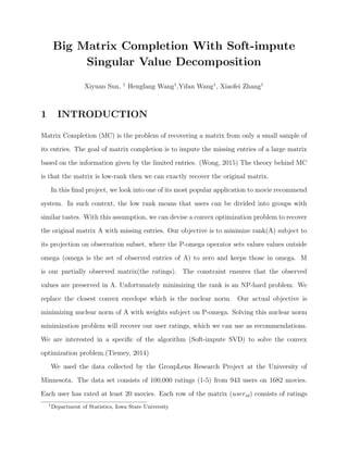
For the Soft-Impute method, we use a equal-spaced grid of 30 λ which is from 30 to 1. For
the svd function irlba, only 82 singular values are used. Below are some results for the
validation step.
(a) (b) (c)
(d) (e)
Figure 1: validation error vs training error via (a) built-in svd; (b) propack.svd; (c) irlba;
(d) fast.svd; (e) RcppAmardillo.
The plots indicate the relationship of training error and validation error are the same for
these five svd methods. That is when the training error increase the validation error first
decrease and then increase.
12

13. Table 5: Comparison for different SVD methods
method built-in svd propack.svd irlba fast.svd RcppAmadillo
time(min) 35.42 42.57 18.65 27.73 42.81
min validation error 0.95178 0.95178 0.95180 0.95178 0.95178
corresponding λ 11 11 11 11 11
test error 0.96426 0.96426 1.03778 0.96426 0.96426
The minimum validation errors of the five methods are almost the same and the λ we
choose for each method are exactly the same. Except for function irlba, the test error are
almost the same for other four svd functions and the test error for function irlba is a little
higher. There are only 82 singular values that are used in the irlba function, so the results
for this method is not as good as others, however, it does not influence the results very much.
When compare the times that each methods used for the algorithm, the irlba is the best.
It is like a kind of trade off between the precision of the reslut and the computation time.
Among the other four methods, fast.svd is the best as the matrix here is ”fat” (943 rows and
1642 columns). The built − insvd is a little better than propack.svd and RcppAmardillo.
13

14. 3.3.1 Bonus
0.2 0.4 0.6 0.8
0.950.960.970.980.991.001.01
100k data using fast SVD
training error
validationerror
Figure 2: Validation RMSE vs. Training RMSE via FRSVT method
By using the method and 100k data, it achieves test error is 0.9344481 when λ is 12. We
choose λ equals to 12 because it achieves lowest validation error. This test error is comparable
with ordinary SVD which is a little surprising because this method uses normal random
number to get SVD. But the time costing is much lower than ordinary method. It spends
14 minutes by using 30 λ from 30 to 1.
We also try other possible way to run it in order to improve the performance. For
example, if the singular value is less than lambda, instead of setting it as zero, I keep it
the same number, the performance did not change too much. If λ is from 1 to 30, the
performance is worse than lambda from 30 to 1. The RMSE will decrease by 0.07. If we
do not center the data to get lsmean for movies or user, the performance is also worse than
centering version. The RMSE will decrease 0.1. The convergence condition also has impact
on the result, the stricter result for convergence rate, the better result it gets. But the time
costing for strict result is much longer. So after balance the RMSE and time, we decide to
select convergence condition is 10−4
. I also try to run it on several ways, but the random
14

15. mechanism in this method have no impact on the result. Every time, it achieves very similar
result. We also tried different tuning parameter in this method and find that it has very
little influence on the result.
References
Raymond K. W. and Thomas C.M. Lee (2015). Matrix Completion with Noisy Entries and
Outliers arXiv:0706.1234 [math.FA]
Hastie, T., Tibshirani, R., & Wainwright, M. (2015). Statistical Learning with Sparsity.
Mazumder, R., Hastie, T. and Tibshirani, R. (2010) Spectral regularization algorithms for
learning large incomplete matrices. Journal of Machine Learning Research, 11, 2287-
2322.
Tiemey, S. (2014, April 4). An Introduction to Matrix Completion. Retrieved May
2, 2016, from SJTRNY: http://sjtrny.com/posts/2014/4/4/an-introduction-to-matrix-
completion.html
15