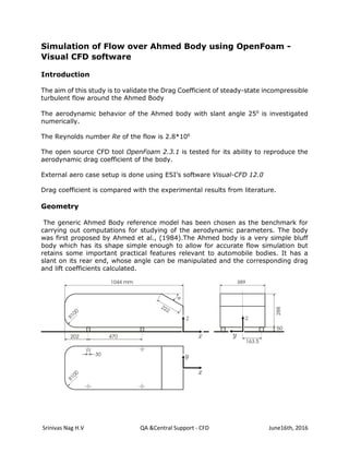
1. Srinivas Nag H.V QA &Central Support - CFD June16th, 2016
Simulation of Flow over Ahmed Body using OpenFoam -
Visual CFD software
Introduction
The aim of this study is to validate the Drag Coefficient of steady-state incompressible
turbulent flow around the Ahmed Body
The aerodynamic behavior of the Ahmed body with slant angle 250
is investigated
numerically.
The Reynolds number Re of the flow is 2.8*106
The open source CFD tool OpenFoam 2.3.1 is tested for its ability to reproduce the
aerodynamic drag coefficient of the body.
External aero case setup is done using ESI’s software Visual-CFD 12.0
Drag coefficient is compared with the experimental results from literature.
Geometry
The generic Ahmed Body reference model has been chosen as the benchmark for
carrying out computations for studying of the aerodynamic parameters. The body
was first proposed by Ahmed et al., (1984).The Ahmed body is a very simple bluff
body which has its shape simple enough to allow for accurate flow simulation but
retains some important practical features relevant to automobile bodies. It has a
slant on its rear end, whose angle can be manipulated and the corresponding drag
and lift coefficients calculated.

2. Srinivas Nag H.V QA &Central Support - CFD June16th, 2016
Geometry of Ahmed Body
Wind Tunnel
STL format of 3D CAD model of Ahmed Body geometry with 250
slant angle is used
for the analysis. Geometry is placed in wind tunnel of dimensions
(15mX1.4mX1.87m) with respect to X, Y and Z directions respectively.
Front space length is kept equal to 3 times the length of geometry and rear space
length is kept 6 times length of geometry.
Wind tunnel has 6 faces namely XMin, XMax, YMin, YMax, ZMin and ZMax.
Geometry is located at ground YMin.
Geometry is mounted on 4 stilts.
Projected area of geometry along positive X direction including stilts is 0.115 m2

3. Srinivas Nag H.V QA &Central Support - CFD June16th, 2016
Wind Tunnel of dimensions (15mX1.4mX1.87m)
Flow Physics
Fluid Properties:
Fluid is Air
Density of the fluid rho = 1.225 kg/m3
Dynamic Viscosity of fluid µ = 1.84*10-5
Ns/m2
Kinematic Viscosity = Dynamic Viscosity/Density = 1.502*10-5
m2
/s
Reynolds number of the flow Re = U*L/ = 2.8*106

4. Srinivas Nag H.V QA &Central Support - CFD June16th, 2016
Boundary Conditions:
Inlet (XMin): Fluid Velocity, U = 40 m/s
Outlet (XMax): No external pressure applied with zeroGradient Velocity
Wall: Geometry Surfaces and Ground (YMin)
Symmetry: ZMin, ZMax and YMax
Time dependence: Steady State analysis.
Turbulence Modelling
Turbulence quantities can be calculated by following formula
Turbulent Kinetic Energy
k = 1.5(UI) 2
I is turbulent intensity in percentage
U is free stream velocity
Energy Dissipation
omega= k0.5
/ (Cu
0.25
*l)
Where Cu is model constant = 0.09
l = length scale which can be estimated as 0.07L.
L is characteristic length
Turbulence quantities used for study are mentioned below
k = 0.287 m2
/s2
, omega = 0.215 s-1
Turbulence model used is kOmegaSST
Spalding Wall functions (nutUSpaldingWallFunction in OpenFoam) is used on Walls.
Y-plus, First cell height and Boundary layers
The near wall region is meshed using the calculated first cell height value with
gradual growth in the mesh so that the viscous effects are captured and avoiding
overall heavy mesh count.

5. Srinivas Nag H.V QA &Central Support - CFD June16th, 2016
Yplus value should be in range 30-300 when Reynolds Average Stress turbulence
(RAS) models are used. There are various Yplus online calculators available. We
have used the one from CFD Online
Mesh definition in Visual CFD
YPlus of 50 was chosen for this study and obtained first cell height (FCH) of 0.478
mm (~0.5mm). This is minimum cell size to be created near walls to accurately
capture viscous effects. This given initial guess for user about the smallest cell size
to be created in computational domain to fairly capture the effects of fluid flow.

6. Srinivas Nag H.V QA &Central Support - CFD June16th, 2016
Boundary layer thickness can be calculated from below formula
δ = x*0.382/Rex
0.2
, where x is the distance in downstream where turbulent boundary
layer starts. Transition to turbulence will be at Re = 10*105
. We have taken total
length of the geometry L = 1.044m and calculated total boundary layer thickness
equal to 15mm.
So, in order to capture turbulent flow accurately, FCH should be within δ=15mm.
Meshing
Base cell size (bsc) is set to 100mm.
‘blockMesh’ utility of OpenFOAM will create a structured hexahedral grid of 100 mm
(bsc) throughout wind tunnel. Output of blockMesh is input to ‘snappyHexMesh’
utility. This creates unstructured polyhedral meshes.
snappyHexMesh works in 3 stages.
1. Snapping: In this stage, fluid mesh is attached to geometry surfaces.
2. Castellation: In this stage, grid refinement occurs.
3. Layer addition: Snapped and Castellated mesh will be projected outwards
from geometry and boundary layers are created near walls.
Total drag force is the summation of Pressure force and Viscous force.
To capture drag due to viscous forces, we have to resolve by creating fine meshes
and boundary layers near walls.
To capture drag due to pressure forces, we have to refine fluid cells in front and
rear part of the geometry. This is done by creating refinement regions
Boundary layers creation
Surface mesh size on walls are set to 3.125mm. FCH in OpenFOAM is based on
surface mesh size. With relative mesh size on, FCH is set to 0.08. This means the
first cell height will be equal to 0.08*3.125 = 0.25mm. Final layer thickness is
1.85mm
12 boundary layers are created with expansion ratio of 1.2. Total boundary
thickness is calculated from geometry progression and equal to 9.89mm. This
covers around 66% of total boundary layer thickness. This should be sufficient to
capture near wall viscous effects.
Another important parameter in creating boundary layers correctly is final layer
ratio which is equal to final layer thickness/surface cell size. This ratio is equal to

7. Srinivas Nag H.V QA &Central Support - CFD June16th, 2016
0.592 in this case. For proper layers to be created, this ratio should be within range
of 0.2 to 0.6.
Boundary layers are created as shown below
Boundary layers generated from snappyHexMesh
Refinement Regions
Cell sizes at a given refinement level ‘n’ is obtained from following equation written
below
CellSize@nth
level = bsc/2n
Say n = 4, then cell size will be equal to 100/24
= 6.25mm
Four refinement regions are created with different levels of refinement as shown in
figure below

8. Srinivas Nag H.V QA &Central Support - CFD June16th, 2016
Refinement Regions

9. Srinivas Nag H.V QA &Central Support - CFD June16th, 2016
Meshing started with 12 cores, 32GB RAM machine.
snappyHexMesh completed meshing within 10 minutes by generating ~4.7 million
cells.
OpenFoam mesh quality criteria is cleared and grid points are transformed to m.
Mesh renumbering is done to reduce band with. This will lead to faster calculation.
Numerical Solver Attributes
For velocity Gauss linearUpwindV scheme is used. For the rest of the variables
upwind schemes are used.
All other attributes are kept with default value of Visual CFD.
Automatic switching of first order schemes to second order is used. Switching is
done after 200 iterations.
First order schemes are numerically stable but less accurate. Second order schemes
are numerically unstable but more accurate. Hence first 200 iterations are run with
first order and switched to second order schemes.

10. Srinivas Nag H.V QA &Central Support - CFD June16th, 2016
Numerical Solver attributes
Force Coefficients Calculation
Force coefficients are calculated by formula
Cd = 2Fd/(rho*A*U2
), where Fd is Drag force and Cd is drag coefficient
Cl= 2Fl/(rho*A*U2
), where Fl is Lift force and Cl is lift coefficient
A is projected area along flow direction.
Force Coefficients inputs

11. Srinivas Nag H.V QA &Central Support - CFD June16th, 2016
Simulation
Flow is initialized using potentialFlow solution. This is done by executing
potentialFoam solver.
simpleFoam solver is run for 5000 iterations.
Results
Velocity Contour

12. Srinivas Nag H.V QA &Central Support - CFD June16th, 2016
Velocity at x=1.244 m (behind slant)

13. Srinivas Nag H.V QA &Central Support - CFD June16th, 2016
Pressure Contour
Total Pressure Coefficient (Cp) distribution in flow field

14. Srinivas Nag H.V QA &Central Support - CFD June16th, 2016
Pressure Contour at x=1.244 m (behind slant)
Pressure Coefficient distribution at x=1.244m (behind slant)

15. Srinivas Nag H.V QA &Central Support - CFD June16th, 2016
Pressure Distribution on Surfaces
Pressure Coefficient Cp distribution on surfaces.

16. Srinivas Nag H.V QA &Central Support - CFD June16th, 2016
Cp = 1 indicates point of stagnation pressure
Cp = 0 indicates that pressure at a point is same as free stream pressure
Cp <1 indicates negative pressure or vacuum
Drag Coefficient (Cd)
Average Drag Coefficient value of last 500 iterations is 0.309.
Experimental Cd value = 0.300.
3% variation is found between experimental Cd and simulation Cd.
Drag Forces
Total force acting on geometry = 34.94 N
Drag Force due to Pressure forces = 29.41 N
Drag Force due to Viscous forces = 5.53 N
From above values is it estimated that approximately 84.17% of total drag forces are
contributed by Pressure Forces and 15.83% of total drag forces are contributed by
Viscous Forces.

17. Srinivas Nag H.V QA &Central Support - CFD June16th, 2016
References
 https://www.learncax.com/knowledge-base/blog/by-category/cfd/basics-of-
y-plus-boundary-layer-and-wall-function-in-turbulent-flows
 http://www.iosrjournals.org/iosr-jmce/papers/vol12-issue4/Version-
3/M012438794.pdf
 http://www.computationalfluiddynamics.com.au/tag/wall-functions/
 http://www.engr.uconn.edu/~wchiu/ME3250FluidDynamicsI/lecture%20note
s/ch09.pdf
 http://www.cfd-online.com/Tools/yplus.php
 http://www.cfd-online.com/Wiki/Y_plus_wall_distance_estimation
 https://en.wikipedia.org/wiki/Boundary_layer_thickness
 https://www.simscale.com/docs/content/validation/AhmedBody/AhmedBody.
html#id7
 CFD Simulation of Flow around External Vehicle: Ahmed Body Saurabh
Banga1, Md. Zunaid2*, Naushad Ahmad Ansari3, Sagar Sharma4, Rohit Singh
Dungriyal5
Pressure and Viscous force contribution on Total Drag
Pressure forces
Viscous Forces

18. Srinivas Nag H.V QA &Central Support - CFD June16th, 2016
 https://en.wikipedia.org/wiki/Turbulence_kinetic_energy
 http://www.cd-
adapco.com/sites/default/files/conference_proceeding/pdf/Ahmed%20Body-
50thAIAA.pdf
 http://www.ijettjournal.org/volume-18/number-7/IJETT-V18P262.pdf
 ERCOFTAC - Ahmed Body experimental values
 http://cfd.mace.manchester.ac.uk/cgi-
bin/cfddb/prpage.cgi?82&EXP&database/cases/case82/Case_data&database/
cases/case82&cas82_head.html&cas82_desc.html&cas82_meth.html&cas82_
data.html&cas82_refs.html&cas82_rsol.html&1&0&0&0&0
 http://cfd.mace.manchester.ac.uk/cgi-
bin/cfddb/prpage.cgi?82&EXP&database/cases/case82/Case_data&database/
cases/case82&cas82_head.html&cas82_desc.html&cas82_meth.html&cas82_
data.html&cas82_refs.html&cas82_rsol.html&1&1&1&1&0&unknown
 http://user.engineering.uiowa.edu/~me_160/lab/cfdefdahmed.pdf
 http://www.taoxing.net/web_documents/cfd_lab4.pdf
 https://www.researchgate.net/publication/282272911_OpenFOAM_step_by_
step_tutorial
 http://cfd.mace.manchester.ac.uk/twiki/pub/Main/TimCraftNotes_All_Access/
advtm-wallfns.pdf
 http://www.cfd-online.com/Wiki/Y_plus_wall_distance_estimation