Who to follow and why: link prediction with explanations
•
6 gefällt mir•1,688 views

Presentation @KDD 2014. In this paper we study link prediction with explanations for user recommendation in social networks. For this problem we propose WTFW (“Who to Follow and Why”), a stochastic topic model for link prediction over directed and nodes-attributed graphs. Our model not only predicts links, but for each predicted link it decides whether it is a “topical” or a “social” link, and depending on this decision it produces a different type of explanation.

Empfohlen
Weitere ähnliche Inhalte
Was ist angesagt?
Was ist angesagt? (20)
Andere mochten auch
Andere mochten auch (20)
Ähnlich wie Who to follow and why: link prediction with explanations
Ähnlich wie Who to follow and why: link prediction with explanations (20)
Kürzlich hochgeladen
Kürzlich hochgeladen (20)
Who to follow and why: link prediction with explanations
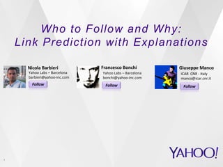
- 1. Who to Follow and Why: Link Prediction with Explanations 1 Nicola Barbieri Yahoo Labs – Barcelona barbieri@yahoo-‐inc.com Follow Francesco Bonchi Yahoo Labs – Barcelona bonchi@yahoo-‐inc.com Follow Giuseppe Manco ICAR CNR -‐ Italy manco@icar.cnr.it Follow This work was partially supported by MULTISENSOR project, funded by the European Commission, under the contract number FP7-610411.
- 2. Motivation § User recommender systems are a key component in any on-line social 2 Given a snapshot of a (social) network, can we infer which new interactions among its members are likely to occur in the near future? Nowell & Kleinberg, 2003 networking platform: § Assist new users in building their network; § Drive engagement and loyalty. Providing explanations in the context of user recommendation systems is still largely underdeveloped !! Who$to$follow!!"!!Refresh! Nicola'Barbieri' Follow% Francesco'Bonchi' Follow% Giuseppe'Manco' Follow%
- 3. Modeling socio-topical relationships ü Has good friends in Barcelona ü Does research on web mining ü Likes blues music 3
- 4. Modeling socio-topical relationships ü Has good friends in Barcelona ü Does research on web mining ü Likes blues music 4 Who$to$follow!!"!!Refresh! Nicola'Barbieri' Follow% Francesco'Bonchi' Follow% Giuseppe'Manco' Follow%
- 5. Modeling socio-topical relationships ü Has good friends in Barcelona ü Does research on web mining ü Likes blues music 5 Who$to$follow!!"!!Refresh! Nicola'Barbieri' Friend!with!@ax,!@bz,!@bcn_fun.! Follow% Francesco'Bonchi' Authorita5ve!about!#YahooLabs,!! #ViralMarke>ng,#WebMining.! Follow% Giuseppe'Manco' Authorita5ve!about!#ClassicRock,!#Blues,!! #Acous>cGuitar.!! Follow%
- 6. Modeling socio-topical relationships ü Has good friends in Barcelona ü Does research on web mining ü Likes blues music 6 Who$to$follow!!"!!Refresh! Nicola'Barbieri' Friend!with!@ax,!@bz,!@bcn_fun.! Follow% Francesco'Bonchi' Authorita5ve!about!#YahooLabs,!! #ViralMarke>ng,#WebMining.! Follow% Giuseppe'Manco' Authorita5ve!about!#ClassicRock,!#Blues,!! #Acous>cGuitar.!! Follow% Common identity and common bond theory: › Identity-based attachment holds when people join a community based on their interest in a well-defined common topic; › Bond-based attachment is driven by personal social relations with other specific individuals.
- 7. Modeling socio-topical relationships ü Has good friends in Barcelona ü Does research on web mining ü Likes blues music 7 Who$to$follow!!"!!Refresh! Nicola'Barbieri' Friend!with!@ax,!@bz,!@bcn_fun.! Follow% Francesco'Bonchi' Authorita5ve!about!#YahooLabs,!! #ViralMarke>ng,#WebMining.! Follow% Giuseppe'Manco' Authorita5ve!about!#ClassicRock,!#Blues,!! #Acous>cGuitar.!! Follow% Identity Bond ✔ ✔ ✔ Common identity and common bond theory: › Identity-based attachment holds when people join a community based on their interest in a well-defined common topic; › Bond-based attachment is driven by personal social relations with other specific individuals.
- 8. Latent factor modeling of socio-topical relationships 8 § Directed attributed-graph § {1,2,3,4,5,6,7} user-set § Links encode following relationships § {a,b,c,d,e,f} features adopted by users E.g. hashtags, tags, products purchased
- 9. Latent factor modeling of socio-topical relationships 9 § 3 communities: § Blue links are bond-based; § Green and orange links are identity-based. § Bond-based communities tend to have high density and reciprocal links § Identity-based communities tend to exhibit a clear directionality
- 10. Latent factor modeling of socio-topical relationships 10 The role and degree of involvement of each user u in the community/topic k is governed by three parameters: Authority – Susceptibility - Social attitude
- 11. Latent factor modeling of socio-topical relationships 11 The role and degree of involvement of each user u in the community/topic k is governed by three parameters: Authority – Susceptibility - Social attitude Authority Susceptibility Social attitude 1 2 3 4 5 6 7 1 2 3 4 5 6 7 1 2 3 4 5 6 7 1 2 3 4 5 6 7 1 2 3 4 5 6 7 1 2 3 4 5 6 7 1 2 3 4 5 6 7 1 2 3 4 5 6 7 1 2 3 4 5 6 7
- 12. Latent factor modeling of socio-topical relationships 12 Identity-based communities tend to have low entropy on the set of features. Authority Susceptibility Social attitude Feature Adoption 1 2 3 4 5 6 7 1 2 3 4 5 6 7 1 2 3 4 5 6 7 1 2 3 4 5 6 7 1 2 3 4 5 6 7 1 2 3 4 5 6 7 a b c d e f a b c d e f 1 2 3 4 5 6 7 1 2 3 4 5 6 7 1 2 3 4 5 6 7 a b c d e f
- 13. WTFW: Generative model 13 1. sample ⇧ ⇠ Dir ⇣ ~⇠ ⌘ 2. For each k 2 {1, . . .,K} sample #k ⇠ Beta(#0, #1) ⌧k ⇠ Beta(⌧0, ⌧1) "k ⇠ Dir (~%) ✓Dir (~↵) ⇣ ⌘ k ⇠ Ak ⇠ Dir ' ~Sk ⇠ Dir (~⌘) 3. For each link l 2 {l1, . . . , lm} to generate: (a) Choose k ⇠ Discrete(⇧) (b) Sample xl ⇠ Bernoulli(#k) (c) if xl = 1 • sample source u ⇠ Discrete(✓k) • sample destination v ⇠ Discrete(✓k) (d) else • sample source u ⇠ Discrete(Sk) • sample destination v ⇠ Discrete(Ak) 4. For each feature pair a 2 {a1, · · · , at} to associate (a) sample k ⇠ Discrete(⇧) (b) Sample ya ⇠ Bernoulli(⌧k): • if ya = 1 then ua ⇠ Discrete(Ak) • otherwise ua ⇠ Discrete(Sk) (c) sample fa ⇠ Discrete("k) Figure 1: Generative process for the WTFW model Following the common identity and common bond theory Authority Interest Social Attitude Feature adoption $ Sk K % & k Ak K K v u xl zl !k K u f za ya # m t ' 0, 1 !0, !1 k !k Community Assignment K K Figure 2: The WTFW model in plate notation. Link labeling Topical role propensity to adopt certain features in F over others. We can formalize such a propensity by means of a weight k,f , denoting the importance of feature f within k.
- 14. Pr(⇥|⌅) represents the product Beta priors. By marginalizing closed form for the joint likelihood The latter is the basis for developing strategy [3, section 11.1.6], where a collapsed Gibbs sampling procedure the matrices Ze,Zf ,X and both the predictive distributions of interest in ⌅. In step consists of a sequential update of the status of the in Ze,Zf ,X and Y. A possible each arc l 2 E and adoption a 2 F chain: Pr(zl = k|Rest),Pr(za = and Pr(ya = 1|Rest)2. By algebraic devise the sampling equations expressed learning scheme is shown in algorithm represent the Gibbs sampling represents the update of the multinomial are collapsed in the derivation of Ak,u = ✓k,if, Conversely, a topical connection l = (u, v) can only be ob-served distributions, a full Bayesian treatment can be obtained by Link prediction if, by picking a latent community k, u has a high Dirichlet and Beta conjugate priors. {⇧, !, ⌧ , ✓,A, S} denote the status of the distri-butions described above. Both the probability of observing degree of activeness Ak,u and v have a high degree of pas-sive Pr(⇥|⌅) represents the Beta priors. By marginalizing closed form for the joint likelihood The latter is the basis strategy [3, section 11.1.6], a collapsed Gibbs sampling the matrices Ze,Zf ,X both the predictive of interest step consists of a sequential of the status in Ze,Zf ,X and Y. each arc l 2 E and adoption chain: Pr(zl = k|Rest),Pr(and Pr(ya = 1|Rest)2. By devise the sampling equations learning scheme is shown algorithm represent the Gibbs represents the update of the are collapsed in the derivation Ak,u = § The probability of observing link l=(u,v) and the adoption of a feature a=(u,f) can be expressed as mixtures over the latent community assignments zl and za: interest Sk,u, that is v) and a feature Pr(l|zl assignment = k, xl = 0,⇥) a = (u, = f) Sk,can u · Ak,be v. ex-pressed mixtures over the latent community assignments Note that the likelihood of observing the reciprocal link u) is equally likely in case of social connection, while it di↵erent in a topical context, and hence reflect our design Pr(l|⇥) = assumption on the directionality of links in social/topical communities. Each link is finally generated by taking into account the social/topical mixture of each community: Pr(l|zl = k,⇥) =!k Pr(l|zl = k, xl = 1,⇥) 14 XK k=1 ⇡k Pr(l|zl = k,⇥) (1) Pr(a|⇥) = XK k=1 ⇡k Pr(a|za = k,⇥) (2) + (1 − !k)Pr(l|zl = k, xl = 0,⇥) generation of a link changes depending on the status cs,s k,u+cs,k,k,u Pr(F|⇥,Y,Zf) = Pr(⇥|⌅) represents the product of Beta priors. By marginalizing over closed form for the joint likelihood Pr(The latter is the basis for developing strategy [3, section 11.1.6], where the a collapsed Gibbs sampling procedure the matrices Ze,Zf ,X and Y, and Social variable xl. A social connection l = (u, v) can observed if, by picking a latent community k, u and degrees of social attitude ✓k,u and ✓k,v, that is Pr(l|zl = k, xl = 1,⇥) = ✓k,u · ✓k,v. a topical connection l = u, v) can only be ob-served by picking a latent community k, u has a high activeness Ak,u and v have a high degree of pas-sive Sk,u, that is Pr(l|zl = k, xl = 0,⇥) = Sk,u · Ak,v. the likelihood of observing the reciprocal link ⌧ dak k (1 − ⌧k)Topical equally likely in case of social connection, while it Pr(E|⇥,X,Z)Pr(Pr(Ze|⇧)Pr(Zf |⇧) Pr(X|Ze, !)Pr(Y|Zwhere cs,s +cs,Pr(E|⇥,X,Ze) = k,uk,k,u Pr(F|⇥,Y,Zf) = Y u Y k ✓ Y u Y k A da k,u k,u S ds k,Pr(Ze|⇧) = Y k ⇡ck k Pr(Zf |⇧) = Y k ⇡dk k Pr(X|Ze, !) = Y k !cs k (1 − !k)k Y Pr(Y|Zf , ⌧) = ⌧ d(1 ⌧k)k − k ak and affinity Topical affinity =!k · ✓k,u · ✓k,v + (1 − !k) · Sk,u · Ak,v Similarly, the probability of observing a node-feature pair = (u, f) 2 F depends on the degree of authoritative-ness/ susceptibility of the user and by the likelihood of ob-serving the attribute f within each latent factor k: Pr(a|za = k,⇥) = (⌧kAk,u + (1 − ⌧k) · Sk,u)#k,f . Here, the term ⌧kAk+(1−⌧k)Sk defines a multinomial distri-bution over users, which encodes the joint (both susceptible and authoritative) attitude of users within that community. 3.1 Learning k and cct ✓k,u = ccdegree of“sociality”!k (or“topicality”, 1−!k) which measures the likelihood of observing social/topical con-nections within each community k; authoritative attitude” ⌧k of observing the adop-tion an attribute by authoritative subject in k (or, the “susceptible attitude”, 1 − ⌧k). whole model relies on multinomial and Bernoulli distributions, a full Bayesian treatment can be obtained by Dirichlet and Beta conjugate priors. {⇧, !, ⌧ , ✓,A, S} denote the status of the distri-butions described above. Both the probability of observing v) and a feature assignment a = (u, f) can be ex-pressed mixtures over the latent community assignments Pr(l|⇥) = XK k=1 ⇡k Pr(l|zl = k,⇥) (1) Pr(a|⇥) = XK k=1 ⇡k Pr(a|za = k,⇥) (2) generation of a link changes depending on the status latent variable xl. A social connection l = (u, v) can observed if, by picking a latent community k, u and degrees of social attitude ✓k,u and ✓k,v, that is Pr(l|zl = k, xl = 1,⇥) = ✓k,u · ✓k,v. a topical connection l = (u, v) can only be ob-served With an abuse of notation, we also introduce described in Tab. 1, relative to these matrices. The key problem in inference is to compute distribution of latent variables given the start by expressing the joint likelihood Pr(E,F,⇥,Ze,Zf ,X,Y|⌅) = Pr(E|⇥,X,Ze)Pr(Pr(Ze|⇧)Pr(Zf |⇧) Pr(X|Ze, !)Pr(Y|where Pr(E|⇥,X,Ze) = Y u Y k ✓ Y u Y k A da k,u k,u S k,Pr(Ze|⇧) = Y k ⇡ck k Pr(Zf |⇧) = Y k ⇡dk k Pr(X|Ze, !) = Y k !cs k (1 − !k)k Y Pr(Y|Zf , ⌧) = k involvement Takes into account the socio-topical tendency of each community It depends on the degree of topical involvement of the user and by the likelihood of observing the feature within k l|· likelihood of observing the reciprocal link equally likely in case of social connection, while it topical context, and hence reflect our design the directionality of links in social/topical Each link is finally generated by taking into social/topical mixture of each community: k,⇥) =!k Pr(l|zl = k, xl = 1,⇥) + (1 − !k)Pr(l|zl = k, xl = 0,⇥) =!k · ✓k,u · ✓k,v + (1 − !k) · Sk,u · Ak,v probability of observing a node-feature pair F depends on the degree of authoritative-ness/ susceptibility of the user and by the likelihood of ob-serving attribute f within each latent factor k: = k,⇥) = (⌧kAk,u + (1 − ⌧k) · Sk,u)#k,f . ⌧kAk+(1−⌧k)Sk defines a multinomial distri-bution users, which encodes the joint (both susceptible authoritative) attitude of users within that community. Learning a collapsed Gibbs sampling the matrices Ze,both the predictive of interest step consists of a sequential of the status in Ze,Zf ,X and each arc l 2 E and adoption chain: Pr(zl = k|Rest),and Pr(ya = 1|Rest)devise the sampling learning scheme algorithm represent represents the update are collapsed in the Ak,by picking a latent community k, u has a high degree of activeness Ak,u and v have a high degree of pas-sive interest Sk,u, that is Pr(l|zl = k, xl = 0,⇥) = Sk,u · Ak,v. Note that the likelihood of observing the reciprocal link v, u) is equally likely in case of social connection, while it di↵erent in a topical context, and hence reflect our design assumption on the directionality of links in social/topical communities. Each link is finally generated by taking into account the social/topical mixture of each community: Pr(l|zl = k,⇥) =!k Pr(l|zl = k, xl = 1,⇥) + (1 − !k)Pr(l|zl = k, xl = 0,⇥) =!k · ✓k,u · ✓k,v + (1 − !k) · Sk,u · Ak,v Similarly, the probability of observing a node-feature pair = (u, f) 2 F depends on the degree of authoritative-ness/ susceptibility of the user and by the likelihood of ob-serving the attribute f within each latent factor k: Pr(a|za = k,⇥) = (⌧kAk,u + (1 − ⌧k) · Sk,u)#k,f . Here, the term ⌧kAk+(1−⌧k)Sk defines a multinomial distri-bution over users, which encodes the joint (both susceptible and authoritative) attitude of users within that community. 3.1 Learning We have described the intuitions behind our joint mod-eling of links and feature associations and now we focus on and ct,d k,u + da ct k + dak + ✓k,u = cs,s k,u + cs,k,2cs k + P Sk,u = ct,s + ds k,u ct + cs + k k dk,+ )
- 15. Link labeling and explanations A social link u → v (u should follow v) is recommended when u and v are Σ Pr( (u→v) is social)∝ π k ⋅δk ⋅θ k,u ⋅θ k,v k § Explanation can be provided as common friends in the communities that better explain the link. 15 both members of at least one social community. A topical link u → v is recommended to (u) when (v) is authoritative in a topic on which (u) has shown interest. Σ Pr( (u→v) is topical)∝ π k ⋅ (1−δk ) ⋅ S k,u ⋅ A k,v k § Explanation as a list of features that characterize the authoritativeness of (v) in (u)’s topics of interest.
- 16. Evaluation model, a recommended 16 § On both Twitter and Flickr the link creation process can be explained in terms of interest identity and/or personal social relations. § Features: § On Twitter: all hashtags and mentions adopted by the user; § On Flickr: all the tags assigned by the user. § Flickr contains ground-truth for the labeling relationships. § Relationships flagged as either “family” or “friends” are labeled as social, the remaining ones as topical. L; explanations for the link. EVALUATION assessment of the The experimen-tation concerns both link the latter refers social or topical. learning procedure, performance varying the sampler. on the internet. As such, it is likely to produce an underes-timation of the accuracy in the label prediction task. In order to keep the experimental setting as close as possi-ble to the original data (high dimensionality and exceptional sparsity), no further pre-processing has been performed. Basic statistics about these two datasets are given in Ta-ble 2. These datasets are characterized by di↵erent prop-erties. The social graph in Twitter is much more directed and sparse than in Flickr, while the number of attributes per user is much higher in Flickr. Twitter Flickr Number of nodes 81, 306 80, 000 Number of links 1, 768, 149 14, 036, 407 Number of one-way links 1, 342, 311 9, 604, 945 Number of bidirectional links 425, 838 4, 431, 462 Number of social links - 6, 747, 085 Number of topical links - 7, 289, 322 Avg in-degree 21 175 Avg out-degree 25 181 Number of features 211, 225 819, 201 Number of feature assignments 1, 102, 000 37, 316, 862 Avg. features per user 15 613 Avg. users per feature 5 45 Table 2: Datasets statistics. Experimental setting. In all the experiments we assume a partial observation of the network and a complete set of user features.4 The learning algorithm starts with a ran-dom assignments to latent variables, it performs a burn-in phase (burn-in=500) to stabilize the Markov chain, and the
- 17. Accuracy on link prediction 17 § Evaluation setting: › On Twitter: Monte Carlo 5 Cross-Validation; › On Flickr: Chronological split. § Negative samples: all the 2-hops non-existing links. § Competitors: › Common neighbors and features; › Adamic-Adar on neighbors and features; › Joint SVD on the combined adjacency/feature matrices
- 18. Flickr: Chronological split. CNF 0.7025/0.7125/0.7199 AA-NF 0.7301/0.7397/0.7472 the 2-hops non-existing links. CNF 0.7025/0.7125/0.7199 AA-NF 0.7301/0.7397/0.7472 AA-NF 0.7301/0.7397/0.7472 Accuracy on link prediction Negative samples: all the 2-hops non-existing links. Table 3: AUC on link prediction - Twitter Competitors: Common neighbors and features; Adamic-Adar; Joint SVD factoriza-tion Number of latent factors Method 8 16 32 64 128 256 WTFW 0.6467 0.6488 0.6534 0.6576 0.661 0.677 JSVD 0.598 0.596 0.597 0.609 0.619 0.624 CNF 0.53 AA-NF 0.58 Table 4: AUC on link prediction - Flickr Number of latent factors Number of latent factors Method 8 16 32 64 128 256 WTFW 0.7393 0.7548 0.7603 0.6883 0.6618 0.6582 Baseline 0.6545 Split 8 16 32 64 128 256 8 16 32 64 128 256 0.567 0.615 0.667 0.707 0.739 0.792 0.565 0.631 0.680 0.713 0.749 0.798 0.586 0.639 0.692 0.732 0.760 0.812 0.439 0.471 0.525 0.588 0.660 0.768 0.446 0.48 0.537 0.602 0.679 0.744 0.454 0.495 0.545 0.617 0.693 0.763 40 0.567 0.615 0.667 0.707 0.739 0.792 30 0.565 0.631 0.680 0.713 0.749 0.798 20 0.586 0.639 0.692 0.732 0.760 0.812 40 0.439 0.471 0.525 0.588 0.660 0.768 30 0.446 0.48 0.537 0.602 0.679 0.744 20 0.454 0.495 0.545 0.617 0.693 0.763 18 X f2F(u)F(v) 1 |V(f)| a matrix factoriza-tion Joint SVD (JSVD) computes a low-rank factor-ization matrix X = [E F] as K is the rank of the square roots of the K Table 3: AUC on link prediction - Twitter Table 3: AUC on link prediction - Twitter Number of latent factors Number of latent factors Method 8 16 32 64 128 256 WTFW 0.6467 0.6488 0.6534 0.6576 0.661 0.677 JSVD 0.598 0.596 0.597 0.609 0.619 0.624 CNF 0.53 AA-NF 0.58 Method 8 16 32 64 128 WTFW 0.6467 0.6488 0.6534 0.6576 0.661 JSVD 0.598 0.596 0.597 0.609 0.619 CNF 0.53 AA-NF 0.58 Table 4: AUC on link prediction - Flickr Table 4: AUC on link prediction - Flickr Number of latent factors Number of latent factors Number of latent factors Method Method 8 8 16 16 32 32 64 64 128 128 256 WTFW WTFW 0.7393 0.7393 0.7548 0.7548 0.7603 0.7603 0.6883 0.6883 0.6618 0.6618 0.6582 Baseline Baseline 0.6545 0.6545 Number of latent factors |N(u) N(v)| + |F(u) Table 5 reports the results for increasing values best results are obtains on a lower number Method Split 8 16 32 64 128 256 WTFW 60/40 0.567 0.615 0.667 0.707 0.739 0.792 Method Split 8 16 32 64 128 256 WTFW 60/40 0.567 0.615 0.667 0.707 0.739 0.792 matrices U and V provide connectivity of both E 70/30 0.565 0.631 0.680 0.713 0.749 0.798 80/20 0.586 0.639 0.692 0.732 0.760 0.812 70/30 0.565 0.631 0.680 0.713 0.749 0.798 80/20 0.586 0.639 0.692 0.732 0.760 0.812 interpreted as the tendency Table 5: AUC on link labeling - Flickr. Table 5: AUC on link labeling - Flickr. JSVD 60/40 0.439 0.471 0.525 0.588 0.660 0.768 JSVD 60/40 0.439 0.471 0.525 0.588 0.660 0.768 70/30 0.446 0.48 0.537 0.602 0.679 0.744 80/20 0.454 0.495 0.545 0.617 0.693 0.763 70/30 Table 0.446 5: AUC 0.48 on link 0.537 labeling 0.602 - Flickr. 0.679 0.744 80/20 0.454 0.495 0.545 0.617 0.693 0.763 adopter in F, relative represents the tendency of We compare the performance of the WTFW model some popular baseline approaches from the literature, perform well on a range of networks [18, 9]: Common Features (CNF) and Adamic-Adar (AA-NF). CNF local similarity index that produces a score for each (u, v), which is given by the number of common features: We compare the performance of the WTFW model with some popular baseline approaches from the literature, which perform well on a range of networks [18, 9]: Common Neigh-bors/ CNF 0.7025/0.7125/0.7199 AA-NF 0.7301/0.7397/0.7472 We compare the performance of the WTFW model with some popular baseline approaches from the literature, which perform well on a range of networks [18, 9]: Common Neigh-bors/ Vf,k represents the The link prediction areas where the JSVD is skewed clearly outperforms the other methods. evident on the Flickr dataset. Evaluation on link labeling. We to the task of discriminating between links, thanks to the ground truth that dataset. Again, we measure the accuracy AUC on the prediction, and by comparing a baseline based on common neighbors/link l = (u, v) is deemed social if the neighbors is higher than those of the topical otherwise. Formally: Number of latent factors N(u) Pr(xl = 1|l) = ||N(u) N(v)| Table 5 reports the results for increasing best results are obtains on a lower in particular for K = 32. This CNF 0.7025/0.7125/0.7199 AA-NF 0.7301/0.7397/0.7472 0.7025/0.7125/0.7199 0.7301/0.7397/0.7472 Table 3: AUC on link prediction - Twitter Table 3: AUC on link prediction - Twitter Features (CNF) and Adamic-Adar (AA-NF). CNF local similarity index that produces a score for each Number of latent factors (u, Number v), which of latent is given factors by the number of common neigh-bors/ Features (CNF) and Adamic-Adar (AA-NF). CNF is a Method 8 16 32 64 128 256 Method 8 16 32 64 128 256 features: features; JSVD) factor-ization as the K provide E tendency relative of the prediction clearly outperforms the other methods. This evident on the Flickr dataset. Evaluation on link labeling. We next turn to the task of discriminating between social links, thanks to the ground truth that we have dataset. Again, we measure the accuracy by computing AUC on the prediction, and by comparing the a baseline based on common neighbors/features. link l = (u, v) is deemed social if the weight of neighbors is higher than those of the common topical otherwise. Formally: Pr(xl = 1|l) = |N(u) N(v)| 0.7025/0.7125/0.7199 0.7301/0.7397/0.7472 Table 3: AUC on link prediction - Twitter AUC on link prediction - Twitter local similarity index that produces a score for each link Figure times AA-NF 0.7301/0.7397/0.7472 Table 3: AUC on link prediction - Twitter Number of latent factors Method 8 16 32 64 128 256 WTFW 0.6467 0.6488 0.6534 0.6576 0.661 0.677 JSVD 0.598 0.596 0.597 0.609 0.619 0.624 CNF 0.53 AA-NF 0.58 Table 4: AUC on link prediction - Flickr Number of latent factors Method 8 16 32 64 128 256 WTFW 0.7393 0.7548 0.7603 0.6883 0.6618 0.6582 Baseline 0.6545 Table 5: AUC on link labeling - Flickr. We compare the performance of the WTFW model with some popular baseline approaches from the literature, which perform well on a range of networks [18, 9]: Common Neigh-bors/ Features (CNF) and Adamic-Adar (AA-NF). CNF is a Figure Figure times
- 19. Link labeling 19 § Baseline on Link Labeling
- 20. Finally, a further assessment of the correct identification 23 25 27 29 31 33 35 37 39 41 43 45 47 49 51 53 55 57 59 61 63 social and topical latent factors can be performed by mea-suring, 51 53 55 57 59 61 63 1 2 3 4 5 6 7 8 9 10 11 12 13 14 15 16 17 18 19 20 21 22 23 24 25 26 27 28 29 30 31 32 assessment of the correct identification latent factors can be performed by mea-suring, feature f, the probability of observing it context, computed as follows: Anecdotal evidence 47 49 51 53 55 57 59 61 63 1 2 3 4 5 6 7 8 9 10 11 12 13 14 15 16 17 18 19 20 21 22 23 24 25 26 27 28 29 30 31 32 evidence for a given feature f, the probability of observing it a social/topical context, computed as follows: Twitter and Flickr, respectively). analysis in Section 4 clearly denotes model to group users according to common features. However, we plan work a more detailed treatment, as well with other approaches in the literature. Second, the approach explored in mixture membership topic modeling. = 0.74 = 0.27 TeamFollow- Back TFB FollowNGain fb InstantFol-lowBack 55 57 59 61 63 1 2 3 4 5 6 7 8 9 10 11 12 13 14 15 16 17 18 19 20 21 22 23 24 25 26 27 28 29 30 31 32 5 6 7 8 9 10 11 12 13 14 15 16 17 18 19 20 21 22 23 24 25 26 27 28 29 30 31 32 Community X each community. f) / ⇡k!k!k,f Feature Prob. Social Feature Prob. Social birthday X k 0.69 hdr 0.40 family 0.67 vintage 0.29 wedding 0.69 collage 0.24 ⇡k(1 − !k)!k,f . party 0.67 nude 0.08 puppy 0.69 polaroid 0.28 f) / k Table 6 we validate the accuracy of the feature-labeling the accuracy of the feature-labeling of tags. The first set contains key-words with social events, such as family, 6: Social/Topical connotations of selected tags on Flickr. task on two small sets of tags. The first set contains key-words Flickr Topic 1 = 0.98 Topic 5 = 0.98 Topic 18 = 0.17 Topic 22 = 0.14 and wedding. The second set contains keywords specific to photographic techniques, e.g. hdr and polaroid, which are likely to generate topical interest in the users. The results confirm the capability of the model to discriminate between social and topical features. Finally, Table 7 summarizes the top keywords detected by our approach on both datasets in some representative com-munities/ second set contains keywords specific to Christmas, techniques, esther, e.g. hdr and polaroid, which are passenger, Birthday, eros, party, stories, apple, topical interest in users. The results the model to discriminate between curling, features. homemade summarizes the top keywords detected by family, mom, dog, driving, vitus, bakery, woods, birthday, friends, halloween, shirt, brothers, baby handmade, warehouse, vintage, knitting, craft, green, pansies, doll, sewing bird, art, design, illustration, drawing, fo-toincatenate, sketch, street, painting, ink, graffiti Twitter datasets in some representative com-munities/ Topic 3 = 0.74 Topic 9 = 0.27 Topic 64 = 0.16 Topic 47 = 0.33 social communities (large !) have e.g., family, christmas on Flickr, characteristic features (e.g., family, christmas on Flickr, and followback on Twitter) which are clearly social. TeamFollow- Back TFB FollowNGain Twitter) InstantFol-lowBack which are clearly social. Autodesk BIM AutoCAD Revit AU2012 Civil3D AEC adsk sf2012 SWTOR revit CAD au2011 cloud 3dsMax ISS space science Discovery Mars nasa spottheshut-tle Game-ofThrones FakeWesteros GoT ooc SXSWesteros TheGhostofHar-renhal CONCLUSIONS AND FUTUREWORK nowplaying lastfm Tea-mAutoFollow CONCLUSIONS AND FUTURE WORK Follow4Follow ESA astronomy Enterprise Gardenof- Bones asoiaf GRRM GOT This paper introduces WTFW, a novel stochastic gener-ative WTFW, a novel stochastic gener-ative factorizes both social connections The model provides accurate link 500aDay anime 4sqDay AU2011 C3D2013 Soyuz and 7: feature 20 Most representative associations. features The model of selected provides communities. accurate link prediction and contextualized socio/topical explanations to Anecdotal evidence notably associated with social events, such as family, model that jointly factorizes both social connections 13 Community 1 2 3 4 5 6 7 8 9 10 11 12 13 14 15 16 17 18 19 20 21 22 23 24 25 26 27 28 29 30 Community 0.0 Figure 9: Distribution of k for each community. k) = Pr(Social |f) / (1 − !k)Ak,u X k ⇡k!k!k,f Pr(Topical |f) / X ⇡k(1 − !k)!k,f . !k✓k,u + (1 − !k)(Ak,u + Sk,u) . k measuring the degree of susceptibility and so-ciality computed likewise. Again, Twitter tends predominant amount of authorities/followers, great majority of the communities in Flickr social users. Finally, Figure 9 shows the of !k within the communities. As already Flickr tends to be more clearly social than Moreover, the distinction between social and topi-cal is very clear in Flickr with almost all com-munities probability of being “social” either above topics: highly social communities (large !) have 0.2. This discriminating attitude is even more increase the number of latent topics. further assessment of the correct identification topical latent factors can be performed by mea-suring, given feature f, the probability of observing it topical context, computed as follows: Social|f) / X Community ⇡!!Feature nowplaying lastfm Tea-mAutoFollow Prob. Social Feature Prob. Social birthday 0.69 hdr 0.40 family 0.67 vintage 0.29 wedding 0.69 Follow4Follow collage 0.24 party 0.67 500aDay nude 0.08 puppy 0.69 anime 4sqDay polaroid 0.28 Table 6: Social/Topical connotations of selected tags on Flickr. Flickr Topic 1 = 0.98 Topic 5 = 0.98 Topic 18 = 0.17 Topic 22 = 0.14 Christmas, esther, passenger, Birthday, eros, party, stories, apple, curling, homemade family, mom, dog, driving, vitus, bakery, woods, birthday, friends, halloween, shirt, brothers, baby handmade, warehouse, vintage, knitting, craft, green, pansies, doll, sewing bird, art, design, illustration, drawing, fo-toincatenate, sketch, street, painting, ink, graffiti Twitter Topic 3 = 0.74 Topic 9 = 0.27 Topic 64 = 0.16 Topic 47 = 0.33 TeamFollow- Back TFB FollowNGain fb InstantFol-lowBack nowplaying lastfm Tea-mAutoFollow Autodesk BIM AutoCAD Revit AU2012 Civil3D AEC adsk sf2012 SWTOR revit ISS space science Discovery Mars nasa spottheshut-tle ESA Game-ofThrones FakeWesteros GoT ooc SXSWesteros TheGhostofHar-renhal Community Community Figure 9: Distribution of k for each community. = (1 − !k)Ak,u !k✓k,u + (1 − !k)(Ak,u + Sk,u) . measuring the degree of susceptibility and so-ciality computed likewise. Again, Twitter tends predominant amount of authorities/followers, majority of the communities in Flickr social users. Finally, Figure 9 shows the !k within the communities. As already Flickr tends to be more clearly social than the distinction between social and topi-cal very clear in Flickr with almost all com-munities probability of being “social” either above This discriminating attitude is even more increase the number of latent topics. assessment of the correct identification latent factors can be performed by mea-suring, feature f, the probability of observing it context, computed as follows: X Social|f) / k ⇡k!k!k,f X Feature Prob. Social Feature Prob. Social birthday 0.69 hdr 0.40 family 0.67 vintage 0.29 wedding 0.69 collage 0.24 party 0.67 nude 0.08 puppy 0.69 polaroid 0.28 Table 6: Social/Topical connotations of selected tags on Flickr. Flickr Topic 1 = 0.98 Topic 5 = 0.98 Topic 18 = 0.17 Topic 22 = 0.14 Christmas, esther, passenger, Birthday, eros, party, stories, apple, curling, homemade family, mom, dog, driving, vitus, bakery, woods, birthday, friends, halloween, shirt, brothers, baby handmade, warehouse, vintage, knitting, craft, green, pansies, doll, sewing bird, art, design, illustration, drawing, fo-toincatenate, sketch, street, painting, ink, graffiti Twitter Topic 3 = 0.74 Topic 9 = 0.27 Topic 64 = 0.16 Topic 47 = 0.33 TeamFollow- Back TFB FollowNGain fb InstantFol-lowBack nowplaying lastfm Tea-mAutoFollow Follow4Follow Autodesk BIM AutoCAD Revit AU2012 Civil3D AEC adsk sf2012 SWTOR revit CAD au2011 cloud 3dsMax ISS space science Discovery Mars nasa spottheshut-tle ESA astronomy Enterprise Game-ofThrones FakeWesteros GoT ooc SXSWesteros TheGhostofHar-renhal Gardenof- 53 55 57 59 61 63 1 2 3 4 5 6 7 8 9 10 11 12 13 14 15 16 17 18 19 20 21 22 23 24 25 26 27 28 29 30 31 32 Community Prob. Social 0.0 0.2 0.4 0.6 Distribution of k for each community. Sk,u) . susceptibility and so-ciality Twitter tends authorities/followers, communities in Flickr shows the As already social than social and topi-cal almost all com-munities either above is even more topics. identification performed by mea-suring, observing it feature-labeling contains key-words Feature Prob. Social Feature Prob. Social birthday 0.69 hdr 0.40 family 0.67 vintage 0.29 wedding 0.69 collage 0.24 party 0.67 nude 0.08 puppy 0.69 polaroid 0.28 Table 6: Social/Topical connotations of selected tags on Flickr. Flickr Topic 1 = 0.98 Topic 5 = 0.98 Topic 18 = 0.17 Topic 22 = 0.14 Christmas, esther, passenger, Birthday, eros, party, stories, apple, curling, homemade family, mom, dog, driving, vitus, bakery, woods, birthday, friends, halloween, shirt, brothers, baby handmade, warehouse, vintage, knitting, craft, green, pansies, doll, sewing bird, art, design, illustration, drawing, fo-toincatenate, sketch, street, painting, ink, graffiti Twitter Topic 3 = 0.74 Topic 9 = 0.27 Topic 64 = 0.16 Topic 47 = 0.33 TeamFollow- Back TFB FollowNGain fb InstantFol-lowBack nowplaying lastfm Tea-mAutoFollow Follow4Follow 500aDay anime 4sqDay Autodesk BIM AutoCAD Revit AU2012 Civil3D AEC adsk sf2012 SWTOR revit CAD au2011 cloud 3dsMax AU2011 C3D2013 ISS space science Discovery Mars nasa spottheshut-tle ESA astronomy Enterprise Soyuz Game-ofThrones FakeWesteros GoT ooc SXSWesteros TheGhostofHar-renhal Gardenof- Bones asoiaf GRRM GOT Table 7: Most representative features of selected communities. Prob. Social 0.0 0.2 0.4 0.6 Distribution of k for each community. Sk,u) . susceptibility and so-ciality Twitter tends authorities/followers, in Flickr shows the As already social than and topi-cal almost all com-munities either above even more topics. identification performed by mea-suring, observing it feature-labeling contains key-words Feature Prob. Social Feature Prob. Social birthday 0.69 hdr 0.40 family 0.67 vintage 0.29 wedding 0.69 collage 0.24 party 0.67 nude 0.08 puppy 0.69 polaroid 0.28 Table 6: Social/Topical connotations of selected tags on Flickr. Flickr Topic 1 = 0.98 Topic 5 = 0.98 Topic 18 = 0.17 Topic 22 = 0.14 Christmas, esther, passenger, Birthday, eros, party, stories, apple, curling, homemade family, mom, dog, driving, vitus, bakery, woods, birthday, friends, halloween, shirt, brothers, baby handmade, warehouse, vintage, knitting, craft, green, pansies, doll, sewing bird, art, design, illustration, drawing, fo-toincatenate, sketch, street, painting, ink, graffiti Twitter Topic 3 = 0.74 Topic 9 = 0.27 Topic 64 = 0.16 Topic 47 = 0.33 TeamFollow- Back TFB FollowNGain fb InstantFol-lowBack nowplaying lastfm Tea-mAutoFollow Follow4Follow 500aDay anime 4sqDay Autodesk BIM AutoCAD Revit AU2012 Civil3D AEC adsk sf2012 SWTOR revit CAD au2011 cloud 3dsMax AU2011 C3D2013 ISS space science Discovery Mars nasa spottheshut-tle ESA astronomy Enterprise Soyuz Game-ofThrones FakeWesteros GoT ooc SXSWesteros TheGhostofHar-renhal Gardenof- Bones asoiaf GRRM GOT Table 7: Most representative features of selected communities. the underlying latent nature behind each observed connec-tion. Autodesk BIM AutoCAD Revit AU2012 Civil3D AEC adsk sf2012 SWTOR revit CAD au2011 cloud 3dsMax AU2011 C3D2013 ISS science Discovery Mars spottheshut-tle astronomy Enterprise Table 7: Most representative features the underlying latent nature behind The result is a decoupling of to reflect the idea that social have high density and reciprocal connections, communities should exhibit clear low entropy over user attributes. Our work can be extended in several deliberately omitted to quantify the that the model produces. Some on modularity look promising (we measured on Community 0.0 Figure 9: Distribution of k for each community. Ak,u Ak,u + Sk,u) . susceptibility and so-ciality Again, Twitter tends authorities/followers, communities in Flickr Figure 9 shows the communities. As already clearly social than between social and topi-cal with almost all com-munities social” either above attitude is even more latent topics. correct identification performed by mea-suring, probability of observing it follows: Feature Prob. Social Feature Prob. Social birthday 0.69 hdr 0.40 family 0.67 vintage 0.29 wedding 0.69 collage 0.24 party 0.67 nude 0.08 puppy 0.69 polaroid 0.28 Table 6: Social/Topical connotations of selected tags on Flickr. Flickr Topic 1 = 0.98 Topic 5 = 0.98 Topic 18 = 0.17 Topic 22 = 0.14 Christmas, esther, passenger, Birthday, eros, party, stories, apple, curling, homemade family, mom, dog, driving, vitus, bakery, woods, birthday, friends, halloween, shirt, brothers, baby handmade, warehouse, vintage, knitting, craft, green, pansies, doll, sewing bird, art, design, illustration, drawing, fo-toincatenate, sketch, street, painting, ink, graffiti Twitter Topic 3 = 0.74 Topic 9 = 0.27 Topic 64 = 0.16 Topic 47 = 0.33 TeamFollow- Back TFB FollowNGain fb InstantFol-lowBack nowplaying Autodesk BIM AutoCAD Revit AU2012 Civil3D AEC adsk sf2012 ISS space science Discovery Mars nasa spottheshut-tle Game-ofThrones FakeWesteros GoT ooc SXSWesteros TheGhostofHar-renhal Community 0.0 Figure 9: Distribution of k for each community. + Sk,u) . susceptibility and so-ciality Twitter tends authorities/followers, communities in Flickr Figure 9 shows the communities. As already clearly social than social and topi-cal almost all com-munities social” either above attitude is even more latent topics. correct identification performed by mea-suring, of observing it follows: Feature Prob. Social Feature Prob. Social birthday 0.69 hdr 0.40 family 0.67 vintage 0.29 wedding 0.69 collage 0.24 party 0.67 nude 0.08 puppy 0.69 polaroid 0.28 Table 6: Social/Topical connotations of selected tags on Flickr. Flickr Topic 1 = 0.98 Topic = 0.98 Topic 18 = 0.17 Topic 22 = 0.14 Christmas, esther, passenger, Birthday, eros, party, stories, apple, curling, homemade family, mom, dog, driving, vitus, bakery, woods, birthday, friends, halloween, shirt, brothers, baby handmade, warehouse, vintage, knitting, craft, green, pansies, doll, sewing bird, art, design, illustration, drawing, fo-toincatenate, sketch, street, painting, ink, graffiti Twitter Topic 3 = 0.74 Topic 9 = 0.27 Topic 64 = 0.16 Topic 47 = 0.33 TeamFollow- Back TFB FollowNGain fb InstantFol-lowBack nowplaying lastfm Tea-mAutoFollow Autodesk BIM AutoCAD Revit AU2012 Civil3D AEC adsk sf2012 SWTOR revit CAD au2011 ISS space science Discovery Mars nasa spottheshut-tle ESA astronomy Game-ofThrones FakeWesteros GoT ooc SXSWesteros TheGhostofHar-renhal Gardenof- 4 5 6 7 8 9 10 11 12 13 14 15 16 17 18 19 20 21 22 23 24 25 26 27 28 29 30 31 32 Community each community. Feature Prob. Social Feature Prob. Social birthday 0.69 hdr 0.40 family 0.67 vintage 0.29 wedding 0.69 collage 0.24 party 0.67 nude 0.08 puppy 0.69 polaroid 0.28 Table 6: Social/Topical connotations of selected tags on Flickr. Flickr Topic 1 = 0.98 Topic 5 = 0.98 Topic 18 = 0.17 Topic 22 = 0.14 Christmas, esther, passenger, Birthday, eros, party, stories, apple, curling, homemade family, mom, dog, driving, vitus, bakery, woods, birthday, friends, halloween, shirt, brothers, baby handmade, warehouse, vintage, knitting, craft, green, pansies, doll, sewing bird, art, design, illustration, drawing, fo-toincatenate, sketch, street, painting, ink, graffiti Twitter Topic 3 = 0.74 Topic 9 = 0.27 Topic 64 = 0.16 Topic 47 = 0.33 TeamFollow- Back TFB FollowNGain InstantFol-lowBack nowplaying lastfm Tea-mAutoFollow Follow4Follow 500aDay anime 4sqDay Autodesk BIM AutoCAD Revit AU2012 Civil3D AEC adsk sf2012 SWTOR revit CAD au2011 cloud 3dsMax AU2011 C3D2013 ISS space science Discovery Mars nasa spottheshut-tle ESA astronomy Enterprise Soyuz Game-ofThrones FakeWesteros GoT ooc SXSWesteros TheGhostofHar-renhal Gardenof- Bones asoiaf GRRM GOT Table 7: Most representative features of selected communities. contextualized socio/topical explanations to Topic 3 = 0.74 Topic 9 = 0.27 Topic 64 = 0.16 Topic 47 = 0.33 TeamFollow- Back TFB FollowNGain fb InstantFol-lowBack nowplaying lastfm Tea-mAutoFollow Follow4Follow 500aDay anime 4sqDay Autodesk BIM AutoCAD Revit AU2012 Civil3D AEC adsk sf2012 SWTOR revit CAD au2011 cloud 3dsMax AU2011 C3D2013 ISS space science Discovery Mars nasa spottheshut-tle ESA astronomy Enterprise Soyuz Game-ofThrones FakeWesteros GoT ooc SXSWesteros TheGhostofHar-renhal Gardenof- Bones asoiaf GRRM GOT Table 7: Most representative features of selected communities. the underlying latent nature behind each observed connec-tion. The result is a decoupling of social and topical con-nections to reflect the idea that social communities should have high density and reciprocal connections, whereas top-ical communities should exhibit clear directionality and low entropy over user attributes. Our work can be extended in several directions. First, we deliberately omitted to quantify the quality of the commu-nities that the model produces. Some initial results based on modularity look promising (we measured 0.55 and 0.37 on Twitter and Flickr, respectively). Also, the qualitative analysis in Section 4 clearly denotes the capability of the model to group users according to both connectivity and common features. However, we plan to devote to future work a more detailed treatment, as well a thorough compar-ison with other approaches in the literature. Second, the approach explored in this paper is rooted on mixture membership topic modeling. However, other alter-natives
- 21. Conclusion and future work 21 § Joint factorization of both social connections and feature associations in a Bayesian framework. § The model provides accurate link prediction and personalized explanations to support recommendations of people to follow. § Future works: › Study user perception of explanations; › Investigate several schemas for generating explanations: • e.g. diversified selection of features/neighbors to cover all communities that better explain the suggested connection › Evaluation in a community detection setting; › Similar characterization in alternative mathematical framework: • e.g. Matrix Factorization.
- 22. 22 Thank you!