This is a basic idea about FDTD Method . I am creating this PPT for my class assignment .Hope This will be helpful for you .Best of luck

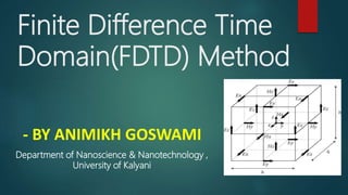
1. Finite Difference Time
Domain(FDTD) Method
- BY ANIMIKH GOSWAMI
Department of Nanoscience & Nanotechnology ,
University of Kalyani

2. Declaimer
Before going to Finite Difference Time Method (FDTD)
(FDTD) we should know about the following topic :
 Vector Algebra and Vector Calculus
 Different form of Maxwell’s equation and their
solving.
 Interpolation and Numerical Analysis
 Finite Difference Method
 Computer Programming
@Animikh Goswami

3. Finite Difference Time Domain Method
Contents :
 Introduction to FDTD
 2D Formulation
 Time Stepping
 Perfectly Matched Layer(PML)
@Animikh Goswami

4. Finite Difference Time Domain Method
(Introduction to FDTD)
History and Central Idea :
 Simplest and most widely used Computational Electromagnetic
method.
 Yee (1966) lead the foundation .
 Very useful for Time domain formulation : Wave Propagation ,
Pulsed transient phenomena . Ex. : Switching .
 Based on differential form of Maxwell’s equation .
@Animikh Goswami

5. Finite Difference Time Domain Method
(Introduction to FDTD)
Assumption :
Linear medium , isotropic , non dispersive .
Maxwell’s Equation :
𝐷 = 𝜀𝐸…………………(1)
𝐵 = 𝜇𝐻 ………………..(2)
𝑑𝐷
𝑑𝑡
= 𝛻 × 𝐻 − 𝐽 .................(3)
𝑑𝐵
𝑑𝑡
= − 𝛻 × 𝐸 ………………(4) @Animikh Goswami

6. Using (1) and (2) equation (3) & (4) can be written as
𝑑𝐷
𝑑𝑡
= 𝛻 × 𝐻 − 𝐽 = 𝜀
𝑑𝐸
𝑑𝑡
................(3)
𝑑𝐵
𝑑𝑡
= − 𝛻 × 𝐸 = 𝜇
𝑑𝐻
𝑑𝑡
………………(4)
 Most of the case in FDTD , we are using in this two equation . In future
we will be used (3) as :
𝑑𝐷
𝑑𝑡
= 𝛻 × 𝐻 = 𝜀
𝑑𝐸
𝑑𝑡
………………(3)
Finite Difference Time Domain Method
(Introduction To FDTD)
@Animikh Goswami

7. Finite Difference Time Domain Method
(Introduction To FDTD)
From Taylor’s series we get :
∆𝑧
2
𝑓′
𝑧0 ≅ 𝑓 𝑧0 +
∆𝑧
2
+ 𝑓 𝑧0 + 0 ∆𝑧2
This is also known as sided differences .
This will be the key term in our FDTD analysis .
@Animikh Goswami

8. Finite Difference Time Domain Method
(2D formulation )
Types of Polarization :
i. Transverse E𝐥𝐞𝐜𝐭𝐫𝐢𝐜 𝑬 𝒙, 𝑬 𝒚, 𝑯 𝒛 :
We are taking Electric field(E) along x and y axis and magnetic(H)
field along perpendicular of them , i.e. z axis .
ii. Transverse Magnetic 𝑯 𝒙, 𝑯 𝒚, 𝑬 𝒛 :
We are taking Magnetic field(H) along x and y axis and Electric(E)
field along perpendicular of them , i.e. z axis .
@Animikh Goswami

9. Finite Difference Time Domain Method
(2D formulation)
Firstly we are taking : TE polarization
From (3) we get: 𝜺
𝝏𝑬 𝒙
𝝏𝒕
=
𝝏𝑯 𝒛
𝝏𝒚
−
𝝏𝑯 𝒚
𝝏𝒛
𝜺
𝝏𝑬 𝒚
𝝏𝒕
=
𝝏𝑯 𝒙
𝝏𝒛
−
𝝏𝑯 𝒛
𝝏𝒙
𝜺
𝝏𝑬 𝒛
𝝏𝒕
=
𝝏𝑯 𝒚
𝝏𝒙
−
𝝏𝑯 𝒙
𝝏𝒚
 since 𝐻 𝑥 = 0 𝑎𝑛𝑑 𝐻 𝑦 = 0 in TE polarization then
𝜺
𝝏𝑬 𝒙
𝝏𝒕
=
𝝏𝑯 𝒛
𝝏𝒚
…………………(5)
𝜺
𝝏𝑬 𝒚
𝝏𝒕
=
𝝏𝑯 𝒙
𝝏𝒛
………………….(6)
@Animikh Goswami

10. Finite Difference Time Domain Method
(2D Formulation )
From (4) we get , 𝛍
𝝏𝑯 𝒛
𝝏𝒕
= − (
𝝏𝑬 𝒙
𝝏𝒚
−
𝝏𝑬 𝒚
𝝏𝒙
) ….................(7)
Convention :
 𝐸 discretized along grid lines (Boundaries )
 𝐻 at centre .
Notation : 𝐸 𝑥 → 𝐸 𝑥 𝑥 = 𝑥0 + ∆𝑥 𝑖 +
1
2
, 𝑦 = 𝑦0 + 𝑗∆𝑦
 Similar case for 𝐸 𝑦 , 𝐻𝑧 .
Grid Calculation :
𝝁𝑯 𝒛 𝒊 +
𝟏
𝟐
, 𝒋 +
𝟏
𝟐
= −
𝑬 𝒙 𝒊 +
𝟏
𝟐
, 𝒋 + 𝟏 − 𝑬 𝒙 𝒊 +
𝟏
𝟐
, 𝒋
∆𝒚
−
𝑬 𝒚 𝒊 + 𝟏, 𝒋 +
𝟏
𝟐
− 𝑬 𝒚 𝒊, 𝒋 +
𝟏
𝟐
∆𝒙
Trick : (top- bottom) and (Left- Right) @Animikh Goswami

11. Finite Difference Time Domain Method
(2D Formulation)
@Animikh Goswami
 Similar formulation can be done for TM polarization method .
TM→ ( 𝐻 𝑥 , 𝐻 𝑦 , 𝐸𝑧)

12. Finite Difference Time Domain Method
(Time Stepping)
Now we are going to Time stepping :
In this methods we are discretizing space & time . So far we are
discussed about Yee cell ( where we used ∆x and ∆y )in space . Now
there will be also a variable , i.e. Time(t). And will be denoted as ∆t .
Notation :
In space the variable was staggered by half a grid (∆x and ∆y ) .
In time variable T will also staggered by half a grid(∆t) .
@Animikh Goswami

13. Finite Difference Time Domain Method
(Time Stepping)
Assumption :
We take the same assumptions is about the medium linear,
homogeneous all of that .
 𝐸 evaluated at integer time grid .
 𝐻 evaluated
1
2
integer gird .
@Animikh Goswami

14. Finite Difference Time Domain Method
(Time Stepping)
Now we take Maxwell’s equation
𝑑𝐷
𝑑𝑡
= 𝛻 × 𝐻 = 𝜀
𝑑𝐸
𝑑𝑡
………………(3)
𝑑𝐵
𝑑𝑡
= − 𝛻 × 𝐸 = 𝜇
𝑑𝐻
𝑑𝑡
………………(4)
From (3) and (4) we get in time domain ,
𝜺
𝑬 𝒏−𝑬 𝒏−𝟏
∆𝒕
= 𝛁 × 𝑯 𝒏−
𝟏
𝟐 ……………..……(8)
μ
𝐻
𝒏+
1
2−𝐻
𝒏−
1
2
∆𝒕
= −𝛁 × 𝐸 𝒏 ……………………(9)
@Animikh Goswami

15. Finite Difference Time Domain Method
(Time Stepping)
From (5) and (6) we get ,
𝑬 𝒏 = 𝑬 𝒏−𝟏 −
∆𝒕
𝜺
𝛁 × 𝑯 𝒏−
𝟏
𝟐 …………………..(10)
𝑯 𝒏+
𝟏
𝟐 = 𝑯 𝒏−
𝟏
𝟐 −
∆𝒕
𝜺
𝛁 × 𝑬 𝒏 ……………............(11)
 Leap Frog Integration Scheme :
Present Past
𝑬 𝑛−1
𝐻 𝑛−
1
2
𝐻 𝑛+
1
2
𝐸 𝑛
𝐸 𝑛+1 t
@Animikh Goswami

16. Finite Difference Time Domain Method
(Graphical Representation of FDTD Simulation)
Cartesian Coordinate System :
yt
x
Yee Cell
@Animikh Goswami

17. Finite Difference Time Domain Method
(Perfectly Matched Layer)
Before going to Perfectly Matched Layer in FDTD ,we should know
about the following topic :
 Accuracy Condition
 Dispersive and Non Dispersive Media
 ABC Implementation in FDTD
 ABC failure in FDTD
@Animikh Goswami

18. Finite Difference Time Domain Method
(Perfectly Matched Layer)
 This is a relatively new development on the Field of FDTD, proposed
by Berenger in 1994.
Advantages (Our wish list for an Absorbing Material based PML ):
1. It observes waves at all angles , so R=0.
2. It works for evanescent waves .
@Animikh Goswami

19. Finite Difference Time Domain Method
(Perfectly Matched Layer)
Schematic Diagram of PML @Animikh Goswami
Wave
Boundary
Absorbing Material
n

20. Finite Difference Time Domain Method
(Perfectly Matched Layer)
1. Normal Incident :
𝑹 =
𝒏−𝟏
𝒏+𝟏
2. Interpretation of PML :
i. Absorbing Material which is anisotropic . ( Physics )
ii. Coordinate Stretching . ( Math ) @Animikh Goswami
Loss
x
Poor Man’s PML
n

21. Finite Difference Time Domain Method
(Perfectly Matched Layer)
From Maxwell’s Equation ( Keep in mind that 𝑗𝜔𝑡 is time dependent ) :
𝛻𝑒 × 𝐸= − j 𝜔𝜇𝐻 ………………(1)
𝛻ℎ × 𝐻 = 𝑗𝜔𝜀𝐸 .................(2)
𝛻𝑒. 𝜀𝐸=ρ …………………(3)
𝛻ℎ. 𝜇𝐻 =0 ………………..(4)
For 1D wave problem we have a solution
𝐸 = 𝐸0 𝑒±𝑗𝑘 𝑟 …………………(5)
We have to find wave propagation vector .
@Animikh Goswami

22. Finite Difference Time Domain Method
(Perfectly Matched Layer)
solving the above equations we get for 1D wave problem
𝑘 𝑧= ℎ 𝑧 𝑒 𝑧
𝜔
𝑐
…………..(6)
Similarly for 3D wave problem we get,
𝑘0
2
=
𝜔
𝑐
2
= 𝑘 𝑒. 𝑘ℎ=
𝑘 𝑥
2
𝑒 𝑥ℎ 𝑥
+
𝑘 𝑦
2
𝑒 𝑦ℎ 𝑦
+
𝑘 𝑧
2
𝑒 𝑧ℎ 𝑧
…………(7)
This is an Ellipsoid . (in polar coordinate system) ,
𝑘 𝑥= ℎ 𝑥 𝑒 𝑥 𝑠𝑖𝑛𝜃𝑐𝑜𝑠𝜑
𝑘 𝑦= ℎ 𝑦 𝑒 𝑦 𝑠𝑖𝑛𝜃𝑠𝑖𝑛𝜑
𝑘 𝑧= ℎ 𝑧 𝑒 𝑧 𝑐𝑜𝑠𝜃
@Animikh Goswami
This is the solution
of (7)

23. Finite Difference Time Domain Method
(Perfectly Matched Layer)
Notation :
1. Set 𝑒 𝑥 = ℎ 𝑥 , 𝑒 𝑦 = ℎ 𝑦 , 𝑒 𝑧 = ℎ 𝑧 called a “Matched” medium. Using
this we get
𝑘 𝑧=𝑘0 𝑒 𝑧 𝑐𝑜𝑠𝜃 (for a Matched medium)
similarly other two .
2. If we make 𝑒 𝑧 to be complex .let 𝑒 𝑧 = 𝑝 + 𝑖𝑞 .
→ 𝑘 𝑧 = 𝑒 𝑗𝑘 𝑧 𝑧 = 𝑒 𝑗𝑘0 𝑒 𝑧 𝑐𝑜𝑠𝜃𝑧
→ 𝑘 𝑧 = 𝑒 𝑗𝑘 𝑧 𝑧 𝑒−𝑗𝑘0 𝑒 𝑧 𝑐𝑜𝑠𝜃𝑧 ( This is known as Evanestcent Wave )
Coordinate Stretching Generating Evanescent wave .
@Animikh Goswami

24. Finite Difference Time Domain Method
Acknowledgement
1. Dr. Ahamed Hossian ( Faculty , Department of
Mathematics , B.K.C.College)
2. Shawon Kumar Awon ( Faculty , Department of
Mathematics , The Heritage College)
3. Subhom Mukherjee
4. Sayon Chakraborty
@Animikh Goswami

25. Finite Difference Time Domain Method
Source :
1. Optical Properties of Metallic Nanoparticles Basic Principles and
Simulation - Andreas Trügler
2. https://en.wikipedia.org/wiki/Finite-difference_time-domain_method#
3. http://www.iitg.ac.in/engfac/krs/public_html/lectures/ee340/FDTD.pdf
@Animikh Goswami

26. Finite Difference Time Domain Method
Thank You
@Animikh Goswami