1. Biodegradable Nanocomposites of Cellulose Acetate
Phthalate and Chitosan Reinforced with Functionalized
Nanoclay: Mechanical, Thermal, and Biodegradability
Studies
Aashish Gaurav,1
A. Ashamol,2
M. V. Deepthi,2
R. R. N. Sailaja2
1
Deparment of Chemical Engineering, IIT, Kharagpur, West Bengal, India
2
The Energy and Resources Institute, Bangalore 560071, Karnataka, India
Received 16 December 2010; accepted 20 July 2011
DOI 10.1002/app.35591
Published online 19 December 2011 in Wiley Online Library (wileyonlinelibrary.com).
ABSTRACT: Biodegradable nanocomposites of cellulose
acetate phthalate and chitosan reinforced with functional-
ized nanoclay (NC) were prepared. The NC loading was
varied from 0 to 10%. The mechanical and thermal prop-
erties have been investigated for these composites. The
nanocomposites exhibited enhanced mechanical proper-
ties due to the addition of NC. The scanning electron
micrographs of the blend specimens also support the
above observations. Thermogravimetric analyses were
carried out to assess the degradation stability of the
blends. The blend shows an increase in the rate of biode-
gradation and water uptake with higher loading of NC.
The exfoliation of NC was analyzed by X-ray diffraction
studies. VC 2011 Wiley Periodicals, Inc. J Appl Polym Sci 125:
E16–E26, 2012
Key words: cellulose acetate phthalate; chitosan; nanoclay;
mechanical and thermal properties; biodegradability
INTRODUCTION
The development of high performance bioplastics is
gaining prominence owing to increasing plastic pollu-
tion and also to conserve the diminishing global petro-
leum reserves. Further, biopolymers are inexpensive,
renewable, and sustainable alternatives, which can
replace petrochemical-derived synthetic polymers.
Cellulose and chitosan are among the most abundant
natural biopolymers, which are inexpensive, renew-
able, and biodegradable with antibacterial properties.
Biobased nanocomposites are produced in which
atleast one component is nanosized and acts as a
reinforcement even with low content.1
Thus, chitosan
reinforced with nanosized cellulose whiskers, which
have been reported to exhibit improved tensile and
water resistance.2
El-Tahlawy et al.3
developed spin-
nable esterified chitosan butyrate/cellulose acetate
blend fibers with enhanced properties. Films of imi-
nochitosan with cellulose acetate yielded smooth ho-
mogeneous films4
with good mechanical strength.
In this study, an esterified cellulose derivative has
been blended with chitosan and reinforced with sur-
face functionalized nanoclay (NC). The mechanical,
thermal, and biodegradability characteristics have
been investigated. It has been found earlier that inter-
actions do exist between chitosan and cellulose as
reported by Hasegawa et al.5
An interpenetrating
polymer network forms between cellulose and chito-
san with decreasing crystallinity as chitosan loading
is increased as reported by Cai and Kim6
An
increased thermal stability of chitosan-montmorillon-
ite biocomposite films dependent of clay content was
reported by Altinisik et al.7
Miscibility studies of chi-
tosan blend with cellulose ethers revealed that the
blends are partially miscible in dry state although,
hydrogen bonding exists between the functionalized
groups.8
However, cellulose acetate/chitosan blend
films have been found to have improved miscibility
and good mechanical properties as studied by Liu
and Bai.9
Similar studies were also reported by Shih
et al.10
Clay reinforced cellulose acetate nanocompo-
sites show an improvement in mechanical properties
and thermal stability.11
In this article, the effect of
adding NC to a blend of cellulose acetate phthalate
(CAP) and chitosan has been investigated. The NC
used is surface modified to enhance dispersion and
bonding with the blend components.
EXPERIMENTAL
Materials
CAP (degree of substitution for acetyl and phthalyl
groups are 1.07 and 0.77, respectively) with
Correspondence to: R. R. N. Sailaja (rrnsb19@rediffmail.
com).
Journal of Applied Polymer Science, Vol. 125, E16–E26 (2012)
VC 2011 Wiley Periodicals, Inc.
2. molecular weight 2534.12 was purchased from GM
Chemicals, Mumbai. Chitosan (with 85% deacetyla-
tion and molecular weight ranging from 10,000 to
15,ooo) was purchased from Marine chemicals, Co-
chin, Kerala. Silane-treated NC was obtained from
Sigma Aldrich (USA). Glycerol and other common
solvents were obtained from S.D. Fine Chem,
Mumbai.
Preparation of blend
A total of 100 g mixture of CAP (60 g) and chitosan
(40 g) powders were taken for the preparation of
composites. NC quantity was varied from 0 to 10 wt
%. The mixture was mixed in a kitchen mixer for 10
min. Glycerol (40% of the weight of the mixture)
was added to the mixture and then sonicated using
Ultra sonicator (Branson, 2510E/DTH) for 30 min.
Water (100 mL) was then added to the mixture and
the contents were kneaded to form a dough. The
blend of pure CAP and chitosan without NC also
contained the same amount of glycerol and water.
The dough samples were kept in zip-locked plastic
packets in refrigerator for further processing.
Compression molding
The dough was partially dried prior to compression
molding. The semi-dried blend was placed in a
mold covered with two polished stainless steel
plates and then compression molded using a locally
fabricated hot press. Sheets were molded at 130
C
under a pressure of 15 MPa for 3 min, and then
cooled to about 50
C for 15 min under constant pres-
sure before releasing the pressure for demolding.
The sheets were then cut into rectangular strips and
these strips were subjected to mechanical testing.
Mechanical properties of the blend
Tensile properties
The tensile properties of the blends were measured
by Zwick UTM (Zwick Roell, ZHU, 2.5) with Instron
tensile flat surface grips at a crosshead speed of 2
mm/min. The tensile tests were performed as per
ASTM D 638 method. The specimens tested were of
rectangular shape having length, width, and thick-
ness of 7, 1.5, and 0.3 cm, respectively. A minimum
of five specimens were tested for each variation in
composition of the blend and results were averaged.
Predictive theoretical models have been used to ana-
lyze the observed experimental results.
Flexural properties
The flexural properties of the blends were measured
by Zwick UTM (Zwick Roell, ZHU, 2.5) with a pre-
load speed of 10 mm/min. The tests were performed
as per ASTM D 790-03 method. The samples were
having a length of 5 cm, width of 2 cm, and a thick-
ness of 0.3 cm. A minimum of five specimens were
tested for each blend and the results were averaged.
Compressive properties
The compressive properties of pure CAP, pure chito-
san, and the blends were performed as per ASTM D
695 by Zwick UTM (Zwick Roell, ZHU, 2.5) with a
preload of 4.5 kN and a test speed of 3 mm/min.
The samples were having a length of 3 cm, width of
2 cm, and a thickness of 0.3 cm. A minimum of five
specimens were tested for each composition and the
results were averaged.
Thermal analysis
Thermogravimetric analysis (TGA) was carried out
for the blends using Perkin-Elmer Pyris Diamond
6000 analyzer in nitrogen atmosphere. The samples
were subjected to a heating rate of 100
C/min in the
heating range of 40–600
C using Al2O3 as the refer-
ence material.
Differential scanning calorimetry (DSC) of the
nanocomposite specimens have been performed in a
Mettler Toledo instrument (model DSC 822e; Mettler
Toledo AG, Switzerland). Samples are placed in
sealed aluminum cells, with a quantity of less than
10 mg and scanning at a heating rate of 10
C/min
up to 250
C.
FTIR spectroscopy
Fourier transform infrared spectroscopy (FTIR; Per-
kin-Elmer spectrum 1000) analysis for the Pure CAP,
chitosan, and the nanocomposites was performed.
X-ray diffraction
XRD measurements for the nanocomposites have
been performed using advanced diffractometer
(PANalytical, XPERT-PRO) equipped with a Cu-ka
radiation source (X ¼ 0.154 mm). The diffraction
data were collected in the 2y range of 3–30
using a
fixed-time mode with a step interval of 0.05
.
Blend morphology
Scanning electron microscopy (SEM; LEICA.S440,
Model 7060) is used to study the morphology of the
fractured and unfractured specimens. The specimens
are gold sputtered prior to microscopy. The SEM
morphology of the unfractured blend specimens was
taken after soaking the samples in dilute sulfuric
STUDY OF FUNCTIONALIZED NANOCLAY E17
Journal of Applied Polymer Science DOI 10.1002/app
3. acid for 24 h and then drying in air after thoroughly
rinsing it in distilled water.
Water absorption
Water absorption index of the samples were meas-
ured according to ASTM D 570-81 with minor modi-
fication.12
The dried sample is weighed and sub-
merged in distilled water at room temperature for
24 h. The extra water on the surface of the specimen
after soaking is removed by placing it in an air oven
at 50
C and the specimen were weighed again. The
container without the soaking specimen is placed in
an air oven at 50
C for 72 h to evaporate the water,
and the water-soluble content obtained was equal to
the increase in container weight. The absorption
(AB) is then calculated by the following eq. (1):
AB ¼ W1 À Wo þ Wsolð Þ=Wo (1)
where W1, Wo, and Wsol are the weight of the speci-
men containing water, the weight of the dried speci-
men, and the weight of the water-soluble residues,
respectively.
Biodegradation
The biodegradation of the blend specimens were car-
ried out by soil burial method.13
Soil-based compost
was taken in small chambers. Humidity of the cham-
bers was maintained at 40–45% by sprinkling water.
The chamber were stored at 30–35
C. Rectangular
specimens were buried completely into the wet soil
at a depth of 10 cm. Samples were removed from the
soil at constant time intervals (15 days) and washed
gently with distilled water and dried in vacuum oven
at 50
C to constant weight. Weight loss percentages
of the samples with respect to time were recorded to
determine the extent of biodegradation.
RESULTS AND DISCUSSIONS
Bionanocomposites of CAP and chitosan have been
prepared and characterized using FTIR, XRD, and
SEM. The mechanical and thermal properties of the
nanocomposites have also been studied.
FTIR spectroscopy
Figure 1 shows the FTIR spectroscopy of neat chito-
san, CAP, and NC, while that of CAP–chitosan nano-
composites are shown in the Figure 2. Spectroscopy
of neat chitosan, CAP, and NC are given for the sake
of comparison. The blends with 0% NC does not
have the peak at 1643 cmÀ1
, which is a characteristic
of amide I band. This is mainly attributed to the fact
that the amide group of chitosan has reacted with the
carboxyl group of CAP. Silanated-NC has two main
peaks. The first one is at 1025 cmÀ1 14
for the Si–O-
stretching of silicate present and also of the interac-
tion with platelet surface. The second peak is at 1603
cmÀ1
for ANH2 (primary amine) stretching, which
does not appear for the blends. The characteristic
bands for CAP at 1035, 1239, 1589, 1724, and 2913
cmÀ1
are respectively for –C–O– stretching, –C–O–C–
stretching, –C¼C– conjugated vinyl aromatic ring, –
C¼O carboxyl group, and asymmetric and symmetric
stretching of methyl –C–H groups.15
All the above
bands are also seen in the blends. However, the other
bands overlap with that of CAP and chitosan.
Stress–strain curves
The engineering stress–strain curves for CAP–chito-
san nanoblends are shown in Figure 3. The stress–
strain curves for neat CAP and chitosan are also
given in the figure for comparison. CAP [curve (a)] is
Figure 1 FTIR Spectra of pure cellulose acetate phthalate,
chitosan, and silanated nanoclay. [Color figure can be
viewed in the online issue, which is available at
wileyonlinelibrary.com.]
Figure 2 FTIR Spectra of CAP–chitosan–nanoclay blends.
[Color figure can be viewed in the online issue, which is
available at wileyonlinelibrary.com.]
E18 GAURAV ET AL.
Journal of Applied Polymer Science DOI 10.1002/app
4. more ductile when compared with chitosan [curve
(b)], which has poor stress resistance and has brittle
characteristics. The blend, however [curve (c)], exhib-
its higher stress value when compared with either of
the blend components. Addition of NC [curve (d)–(f)]
improves both stress as well as strain values owing
to its reinforcing effect among the blend components.
The optimal stress values at 6% NC [curve (g)]
shows, values higher than either CAP or chitosan
with a strain values higher than that of chitosan.
However, higher loading of NC of 10% [curve (h)]
has a detrimental effect on the mechanical properties
of the blend. This may be due to saturation of reac-
tive sites of CAP or chitosan, which can react with
the amine group of silane-treated NC. Thus, excess
NC behaves like a separate third phase, which
reduces the properties.
Effect of NC addition on mechanical properties
Tensile properties
Figure 4 shows the plot of relative tensile properties
(i.e., relative to blend without NC) versus volume
fraction of NC (/). The relative elongation at break
(REB) increases by adding NC up to / ¼ 1.0147 (i.e.,
6% NC) and reaches an optimal value of 1.8. This is
contrary to the expectation that the addition of rigid
NC particles had to lower the REB values and, in
this case, the elongation at break values are even
higher than either CAP or chitosan. A similar obser-
vation was made by Balakrishnan et al.16
. Sue
et al.17
also did not observe a lowering in strain
by adding rigid zirconium phosphate particles,
although the mechanism is not well understood. It
may be due to the fact that the amine group of sil-
ane-treated NC gets coated/interacted with CAP
and the plastic deformation gets initiated around the
blend particles. CAP is relatively more ductile than
chitosan and NC, and this also helps in further
anchoring the two blend components.
Figure 3 Plots of engineering stress–strain curves for
pure cellulose acetate phthalate, chitosan, and CAP–chito-
san–nanoclay blends.
Figure 4 Plots of relative tensile properties versus vol-
ume fraction of nanoclay. (a) Relative tensile strength, (b)
relative Young’s modulus, (c) relative elongation at break.
[Color figure can be viewed in the online issue, which is
available at wileyonlinelibrary.com.]
STUDY OF FUNCTIONALIZED NANOCLAY E19
Journal of Applied Polymer Science DOI 10.1002/app
5. The relative tensile strength (RTS) of the nanocom-
posites also showed a 10% increase when compared
with blends without NC. The optimal value is
reached at / ¼ 1.0147 (i.e., 6% NC loading) beyond,
which it is detrimental for the nanoblends. It may be
due to the fact that all the reactive sites have been
used up to this NC loading and with further NC
loading, they agglomerate due to the presence of
excess unreacted sites.
The relative tensile modulus (RYM) values also
reduce due to the addition of NC and the curve is a
mirror image of that obtained for REB, although in
most cases, the addition of rigid particles such as
starch to a ductile matrix exhibits an increase in
modulus.18
To further analyze the obtained experimental
results, the following predictive theories have been
used as described below.
Figure 4(a) shows the plot of RTS values versus
volume fraction of NC (/). The volume fraction of
NC, was calculated using the following eq. (2):
/i ¼
wi=qið Þ
P
wi=qið Þ
(2)
In eq. (2) wi and qi is the weight fraction and den-
sity of component i in the blend. The density values
of CAP, chitosan, and NC have been measured to be
0.92, 0.54, and 0.36 g/cm3
, respectively.
Three models were used to compare the obtained
experimental tensile strength values. The first is the
Nicolais and Narkis model,19
which is as follows.
RTS ¼
rb
ro
¼ 1 À 1:21/2=3
(3)
In eq. (3), rb and rO are the tensile strength of the
nanoblends and tensile strength of the blend without
NC reinforcement. The model assumes that addition
of filler reduces the effective cross-sectional area and
there exists no adhesion between filler and matrix.
As observed in plot 4(a), the theoretical values of eq.
(3) and the experimental RTS values does not match.
The second model is the Halpin–Tsai model,19
which is given below in eq. (4)
RTS ¼
rb
ro
¼
1 þ GgT/
1 À gT/
(4)
In eq. (4), gT is given by the following equation.
gT ¼
RT À 1
RT þ G
and G ¼
7 À 5t
8 À 10t
(5)
In eq. (5), RT is the ratio of tensile strength of NC
to the tensile strength of CAP/chitosan blend with-
out NC. RT was determined by trial and error by
minimizing the difference between the obtained ex-
perimental results and calculated theoretical values,
this was found to be 0.548. t is the Poisson’s ratio of
CAP/chitosan blend, which is taken to be 0.37.20
The predicted values obtained from eq. (5) are closer
to the experimental values when compared with that
obtained by Nicolais–Narkis model, as the Halpin–
Tsai model assumes good adhesion between the
blend components.
The third model is the Turcsanyi model,21
which
includes an interfacial parameter B, which is a mea-
sure of extent of adhesion of the filler with the ma-
trix and the equation, is given below as follows.
RTS ¼
rb
ro
¼
1 À /
1 þ 2:5/
expðB/Þ (6)
The value of B was determined to match with the
experimental results and this was found to be 2.4,
which indicates good adhesion. The amine group of
silane on NC interacts well with the blend compo-
nents and thus leads to enhanced tensile strength
values. A similar analysis using the above model
was carried out by Zou et al.22
for polyesteramide
composites with different fillers. Thus, blends with
poor tensile strength showed a B value of 0.25 (no
adhesion), while higher values (e.g., 3.44 for talc)
indicated better adhesion. The values obtained for
eq. (6) are also shown in Figure 4(a). The predicted
values of the Turcsanyi model are higher than that
obtained for eq. (3), but theoretical values obtained
from Halpin–Tsai model are closer to the experimen-
tal data.
Figure 4(b) shows a plot of relative tensile modu-
lus (RYM) versus volume fraction of NC. The RYM
values reduce with the increase in NC content as
described earlier.
Three models have been used to analyze the
obtained experimental data. The first is the Kerner’s
model,19
which assumes no interaction between the
blend components and is given by:
Eb
Eo
¼ RYM ¼ 1 þ
/
1 À /
15 1 À tð Þ
ð8 À 10tÞ
(7)
In eq. (7), Eb and EO are the tensile modulus of the
nanoblends and that of the CAP–chitosan blend
without NC, respectively.
The theoretical values obtained from eq. (7) are
also plotted in Figure 4(b). The experimental data
does not match with the predicted values indicating
the existence of interaction between the blend com-
ponents. The model for improved matrix–filler inter-
action is described by the Halpin–Tsai model given
below in eq. (8).
RYM ¼
1 þ gm/
1 À gm/
(8)
E20 GAURAV ET AL.
Journal of Applied Polymer Science DOI 10.1002/app
6. where gm is given by:
gm ¼
Rm À 1
Rm þ G
(9)
In eq. (9), Rm is the ratio of filler modulus to ma-
trix modulus. Rm was determined by trial and error
to match with the experimental results as described
earlier and was found to be 0.004. The values deter-
mined using eq. (8) is also plotted in Figure 4(b).
The predicted values are closer to the experimental
data and the trend also matches with that obtained
experimental results.
The third model is the one developed by Sato and
Furukawa,21
which includes an adhesion parameter
n, which varies from 0 to 1 for perfect adhesion to
no adhesion. The model is described by eq. (10)
below.
RYM ¼ ð1 þ
/2=3
2 À 2/1=3
!
1 À wnð Þ À
/2=3
wf
1 À /1=3
/
2
4
3
5
(10)
where,
w ¼
/
3
1 þ /1=3
À /2=3
1 À /1=3
þ /2=3
!
(11)
The value of n was determined to match with the
experimental results and has been found to be 0.7.
The value of n indicates good adhesion and is
between the two extremes. The theoretical data pre-
dicted using eq. (10) show a trend similar to that
experimentally observed as shown in Figure 4(b).
Figure 4(c) shows a plot of REB versus volume
fraction (/) of NC. As observed earlier, there is a
significant improvement in REB values by the addi-
tion of NC. Nielsen’s model23
has been used to ana-
lyze the observed values. The equation for this
model is given below.
REB ¼
2b
2o
¼ 1 À k/
2=3
(12)
In eq. (12), eb and eO is the elongation at break for
the nanoblends and that of the blend without NC,
respectively. In eq. (12), k is an adjustable parameter,
which depends on filler geometry. The value of k
was computed by trial and error to get the best
match for the obtained experimental results and this
was found to be 0.09. The theoretical values plotted
in Figure 4(c) do not match with the experimental
values, which indicate that this model cannot
explain the observed trend.
Compressive properties
Figure 5(a) shows a plot of relative compressive
strength (RCS) of the blends versus percentage NC
loading. The RCS value reaches an optimal value at
6% NC loading and the compressive strength of the
blend increases by 22% (RCS ¼ 1.22) when com-
pared with blend without NC. The compressive
strength of the blends reduce due to the addition of
chitosan as it is brittle compared with CAP (the
compressive strength of CAP is 12.96 Mpa). The
nonlinearity of compressive properties has been dis-
cussed by Siqueira et al.24
A threefold increase in
compressive properties for biocompatible nanocom-
posites has been observed by Shi et al.25
Figure 5(b) shows the plot of relative compressive
modulus (RCM) versus percentage NC loading for
CAP–chitosan blends. The RCM values show a
decreasing trend with the addition of functionalized
Figure 5 Variation of relative compressive properties
with percentage nanoclay. (a) Relative compressive
strength, (b) relative compressive modulus. [Color figure
can be viewed in the online issue, which is available at
wileyonlinelibrary.com.]
STUDY OF FUNCTIONALIZED NANOCLAY E21
Journal of Applied Polymer Science DOI 10.1002/app
7. NC. The RCM values slightly reduce from 1.0 (with-
out NC) to 0.947 with 6% NC as the optimal value.
The plasticizing effect of ester group also plays a
role in the reduction of modulus values as esters
behave like internal plasticizers.26
Flexural properties
Figure 6(a) shows the relative flexural strength (RFS)
for the blends versus percentage NC loading. Addi-
tion of NC to the blend did not show any improve-
ment of RFS values. The RFS value for blend with 3,
6, and 8% NC were, respectively, found to be 0.966,
0.95, and 0.996.
Figure 6(b) show the relative flexural modulus
(RFM) versus %NC loading. The blend containing
no NC has a RFM-value of 1.0, while an optimal
value of 1.014 was observed with 6% NC. Thus, in
Figure 6 Variation of relative flexural properties with
percentage nanoclay. (a) Relative flexural strength, (b) rela-
tive flexural modulus. [Color figure can be viewed in the
online issue, which is available at wileyonlinelibrary.com.]
Figure 7 TGA themograms of pure CAP, chitosan, CAP–
chitosan–nanoclay blends.
Figure 8 DSC thermograms for pure CAP, chitosan,
CAP–chitosan–nanoclay blends. [Color figure can be
viewed in the online issue, which is available at
wileyonlinelibrary.com.]
E22 GAURAV ET AL.
Journal of Applied Polymer Science DOI 10.1002/app
8. general, the flexural properties did not exhibit any
improvement on NC addition. Sorrentino et al.27
suggested that the enhancement of flexural proper-
ties is mainly due to the formation of three dimen-
sional network of silicate layers. Similar observation
for soy-based nanocomposites has been reported by
Sithique et al.28
Thermogravimetric analysis
Figure 7 shows the TGA thermograms of CAP–chito-
san blends. The thermograms for neat CAP, chito-
san, and NC are also included in the figure for the
sake of comparison.
Neat CAP [curve (a)] shows a main degradation
peak at 310
C (with 78.1% weight loss) with a
shoulder peak at 249
C (with 40.7% weight loss). At
this temperature, elimination of acetyl and phthalyl
groups takes place and the onset of backbone chain
degradation takes place29
and at 376
C, 99% weight
loss occurs. Chitosan [curve (b)] undergoes a single
stage degradation at 290.5
C (with 54.7% weight
loss) owing to the degradation and deacetylation of
chitosan.30
Among the CAP and chitosan, the latter has a bet-
ter thermal stability probably owing to inter- and
intramolecular hydrogen bonding. Similar observa-
tions have been reported by various authors.31–33
The blends of CAP and chitosan [curve (c)] exhibit
better interaction with only 47% weight loss at
310
C. Addition of NC slightly enhanced the ther-
mal stability and an increase in char content was
observed [curves (d) and (e)].
DSC thermograms
The DSC thermograms for CAP–chitosan blends are
shown in Figure 8(a). Pure CAP shows a Tg at
Figure 9 XRD spectra of pure CAP, chitosan, CAP–chito-
san–nanoclay blends. [Color figure can be viewed in the
online issue, which is available at wileyonlinelibrary.com.]
Figure 10 Scanning electron micrographs showing blend
morphology for CAP–chitosan–NC. (a) CAP–chitosan
blend without NC, (b) CAP–chitosan blend with 10% NC.
STUDY OF FUNCTIONALIZED NANOCLAY E23
Journal of Applied Polymer Science DOI 10.1002/app
9. 146
C. Similar observations have been reported by
Rao et al.34,35
The Tg of pure chitosan is at 142
C,
which agrees with the results of Dong et al.36
Another transition at 228
C may be attributed to liq-
uid–liquid transition.36
The composites without NC
(0% NC) show a Tg at 140
C. Addition of 2 and 8%
NC shows a Tg at 142.2 and 143
C, respectively.
Thus, the Tg values for the blends are between the
two extremes, i.e., between that of neat CAP and
neat chitosan.
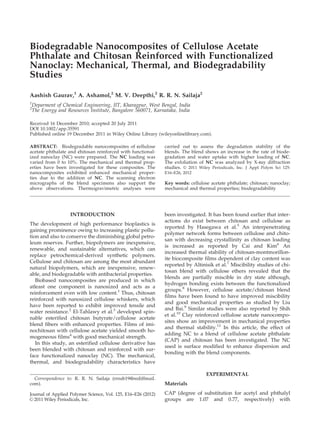
Figure 11 Scanning electron micrographs showing tensile fracture morphology for CAP–chitosan–NC. (a) Neat chitosan,
(b) neat CAP, (c) CAP–chitosan blend without NC, (d) CAP–chitosan blend with 6% NC, (e) CAP–chitosan blend with
10% NC.
E24 GAURAV ET AL.
Journal of Applied Polymer Science DOI 10.1002/app
10. X-ray diffraction
The XRD patterns of CAP–chitosan biocomposites
are shown in Figure 9. This figure also includes the
XRD profiles for neat NC, CAP, and chitosan.
Neat NC indicates a characteristic diffraction at 2y
values of 8.03
, 19.778
, 24.73
, and 26.63
. Neat CAP
has a main broad peak at a 2y value of 22.038
,
while that for chitosan the crystalline peak is at
20.792
. The blend of CAP and chitosan (without
NC) has a peak at a 2y value of 19.5574
accompa-
nied by a small shoulder peak at 22
. The curve for
blend loaded with 3% NC and 6% NC is also shown
in Figure 9. The characteristic peak at 8.03
of NC is
missing indicating that NC has formed an exfoliated
structure with the blend components. Similar obser-
vation has been made for chitosan-based nanocom-
posites as reported by Wang and Wang.37
Blend morphology
Figure 10 shows the blend morphology of CAP–chito-
san blend. The samples were etched in acid solution
for 3 h so that the chitosan phase is removed. Figure
10(a) shows the morphology of CAP–chitosan blends.
The morphology shows a highly deformed matrix as
CAP and chitosan form partially miscible blends. It
also includes a large number of elongated voids indi-
cating resistance to removal of chitosan from the ma-
trix. Figure 10(b) shows the morphology for blends
containing 10% NC. The surface shows a large number
of elongated voids caused by the debonded particles
spread through the entire surface area. The elongated
voids indicate deformation of the matrix and hence
the resistance for removal of particles. Thus, the modi-
fied NC has dispersed uniformly in the entire surface.
Figure 11(a)–(e) shows the tensile fracture mor-
phology of CAP–chitosan blends using SEM. Figure
11(a) shows the fractured SEM micrograph of neat
chitosan. The micrograph shows a dense homogene-
ous structure with brittle characteristics, while that
for CAP [Figure 11(b)] shows a sheared matrix with
elongated voids due to tearing which indicates
higher ductility when compared with chitosan. The
blend without NC [Figure 11(c)] shows brittle failure
characterized by sheared matrix accompanied by
cavities left by debonded particles indicating the
interactions between CAP and chitosan. Similar
observations for chitosan blends with cellulose
ethers were reported by Yin et al.8
The SEM micrograph of the tensile fractured sur-
face of the blend containing 6% NC is shown in [Fig-
ure 11(d)]. The micrograph shows a dense homoge-
neous interlocked surface with a large number of
elongated voids left by debonded particles. The
numbers of voids were found to increase at higher
filler content as shown in Figure 11(e).
Water uptake
Table I shows the values of water absorption charac-
teristics of CAP–chitosan blends. chitosan and CAP
have similar water uptake characteristics (i.e., 70.07
and 68.07%, respectively). The blends (with no NC)
have a water uptake of 22.21%. This may be due to
the interactions between CAP and chitosan, which
form a network. The addition of NC up to 3% fur-
ther reduces water absorbance as clay acts as a me-
chanical barrier. Addition of NC has further
improved the water barrier properties owing to the
tortuous path taken by the fluid and water absorp-
tion further drops down to 14.28%. However, at
higher content of NC (4%), the water absorbency
increases. This may be due to the interaction
between the excess amine groups on the NC surface
with CAP and chitosan leading to a polymeric net-
work. A similar observation was made by Zhang
et al.,38
in which case the surface groups of the clay-
like material interacted with modified chitosan lead-
ing to an increase in water absorbency.
Biodegradation studies
Figure 12 shows the plot of percentage weight loss
versus number of days for the CAP–chitosan blends.
Chitosan is more biodegradable than CAP as the
hydroxyl groups in the latter are replaced by ester
groups. The blends show a retarded degradation for
the first 3 days but, thereafter, the biodegradation is
higher than either CAP or chitosan as observed in
the first 30 days. The addition of NC further lowers
the biodegradation up to 4% NC loading. This may
be due to the interaction between CAP and chitosan
with the amine groups of modified NC, which
restricts the segmental motion at the interface caus-
ing the effective path length and diffusion time to
increase. A similar observation has been made by
Rindusit et al.39
for methylcellulose–montmorillonite
(MMT) composites.
However, beyond 4% NC, the blend exhibits a
higher degradation than for lower NC loadings. The
addition of increased modified NC induced large
TABLE I
Variation of Water Uptake of Neat CAP, Chitosan, and
CAP–Chitosan–NC blends
Sample NC (%) Water absorption (%)
CAP 68.07
Chitosan 70.07
NC0 22.21
NC2 17.70
NC3 14.28
NC4 20.27
NC6 23.52
NC8 19.49
NC10 22.86
STUDY OF FUNCTIONALIZED NANOCLAY E25
Journal of Applied Polymer Science DOI 10.1002/app
11. amorphous regions and these regions are easily ac-
cessible during the degradation process. A similar
observation was made by Wu and Wu,40
when the
biodegradation rates increased with 6% MMT when
compared with 3% MMT loading.
Further, there is an interrelation between water
uptake and degradability as higher water uptake
accelerates the degradation process. Thus, increase
in hydrophilicity increase leads to an increase in bio-
degradability. Thus, for water uptake, the blends
loaded with lower content of NC show a lower
uptake while blends loaded with 4% NC show
increased water absorption characteristics and hence
higher biodegradability.
CONCLUSIONS
CAP has been blended with chitosan along with
modified NC as reinforcing filler. The mechanical and
thermal properties were examined for NC variation.
The tensile strength reached an optimal value with
6% NC. The tensile modulus reduces as NC loading
increases, while the elongation at break increases.
Theoretical models used to analyze the obtained ex-
perimental values indicated interactions between the
blend components. Compressive strength improved
by 22% by the addition of NC, while the flexural
properties were unaffected for the nanocomposites.
Addition of NC enhanced the thermal stability as
indicated by an increase in char content. XRD studies
revealed exfoliation of NC in the blend. Water uptake
reduced to 14.28% on adding NC to the blends.
The authors thank the Department of Science and Technol-
ogy (DST) for the financial assistance for carrying out this
work under the Green Chemistry Programme (2007–2010).
References
1. Angles, M. N.; Dufresne A. Macromolecules 2008, 33, 8344.
2. Li, Q.; Zhou, J.; Zhang, L. J Polym Sci B Polym Phys 2009, 47,
1069.
3. El-Tahlawy, K.; Hudson, S. M.; Hebeish, A. A. J Appl Polym
Sci 2007, 105, 2801.
4. El-Tahlawy, K.; Abdelhaleem, E.; Hudson, S. M.; Hebeish, A.
J Appl Polym Sci 2007, 104, 727.
5. Hasegawa, M.; Isogai, A.; Onabe, F.; Usuda, M.; Atalla, R. H.
J Appl Polym Sci 1995, 45, 1873.
6. Cai, Z.; Kim, J. J Appl Polym Sci 2009, 114, 280.
7. Altinisik, A.; Seki, Y.; Yurdakoc, K. Polym Compos 2009, 30,
1035.
8. Yin, J.; Lao, K.; Chen, X.; Khutoryanspiy, V. V. Carbohydr
Polym 2006, 63, 238.
9. Liu, C.; Bai, R. J Membr Sci 2005, 267, 68.
10. Shih, C.; Shieh, Y.; Twn, Y. Carbohydr Polym 2009, 79, 169.
11. Wibowo, A. C.; Misra, M.; Park, H. M.; Drzal, R. S.; Mohanty,
A. K. Compos A Appl Sci Manuf 2006, 37, 1428.
12. Huang, J.; Zhang, L.; Wang, X. J Appl Polym Sci 2003, 89, 1685.
13. Goswami, T. H.; Maiti, M. M. Polym Degrad Stabil 1998, 61,
335.
14. Shanmugharaj, A. M.; Rhee, K. Y.; Ryu, S. H. J Colloid Inter-
face Sci 2006, 298, 854.
15. Menjoge, A. R.; Kulkarni, M. G. Int J Pharm 2007, 343, 106.
16. Balakrishnan, S.; Start, P. R.; Raghavan, D.; Hudson, S. D.
Polymer 2005, 46, 11255.
17. Sue, H. J.; Gam, K. T.; Bestaoul, N.; Suprr, N.; Clearfield, A.
Chem Mater 2004, 16, 242.
18. Sailaja, R. R. N.; Chanda, M. J. Appl Polym Sci 2001, 80, 863.
19. Willett, J. L. J Appl Polym Sci 1994, 54, 1685.
20. Bliznakov, E. D.; White, C. C.; Shaw, M. T. J Appl Polym Sci
2000, 77, 3220.
21. Hsieh, C. L.; Tuan, W. H. Mater Sci Eng 2005, 396, 202.
22. Zou, Y.; Wang, L.; Zhang, H.; Qian, Z.; Mou, L.; Wang, J.; Liu,
X. Polym Degrad Stabil 2007, 83, 87.
23. Isabella, F.; Micheline, B.; Alain, M. Polymer 1998, 39, 4773.
24. Siqueira, G.; Bras, J.; Dufresne, A. Polymer 2010, 2, 728.
25. Shi, X.; Hudson, J. L.; Spicer, P. P.; Tour, J. M.; Krishnamoorti,
R.; Mikos, G. Biomacromolecules 2006, 7, 2237.
26. Sagar, A. D.; Merrill, E. W. J Appl Polym Sci 1995, 58, 1647.
27. Sorrentino, A.; Gorasi, G.; Vittoria, V. Trends Food Sci Technol
2007, 18, 84.
28. Sithique, M. A.; Alagar, M.; Ali Khan. F. L.; Nazeer, K. P.
Malays Polym J 2011, 6, 1.
29. Tserki, V.; Matzinos, P.; Koppon, S.; Panayiotou, C. Compos A
2005, 36, 965.
30. Tserki, V.; Matzinos, M.; Panayiotou, C. Compos A 2006, 37,
1231.
31. El-Hefian, E. A.; Naset, M. M.; Yahaya, A. H. J Chem 2010, 7,
1212.
32. He, L.; Xue, R.; Yang, D.; Liu, Y.; Song, R. Chin J Polym Sci
2009, 27, 501.
33. Duan, W.; Chen, C.; Jiang, L.; Li, G. H. Carbohydr Polym
2008, 73, 582.
34. Rao, V.; Ashokan, P. V.; Shridhar, M. H. J Appl Polym Sci
2000, 76, 859.
35. Rao, V.; Ashokan, P. V.; Amar, J. V. J Appl Polym Sci 2002,
86, 1702.
36. Dong, Y.; Rwan, Y.; Wang, H.; Zhao, Y.; Bi, D. J Appl Polym
Sci 2004, 93, 1553.
37. Wang, L.; Wang, A. J Hazard Mater 2007, 147, 979.
38. Zhang, J.; Wang, Q.; Wang, A. Carbohydr Polym 2007, 68,
367.
39. Rindusit, S.; Jingjid, S.; Damrongsappul, S.; Tiptikaporn, S.;
Tapeichi, T. Carbohydr Polym 2008, 72, 444.
40. Wu, T.; Wu, C. Polym Degrad Stabil 2006, 91, 2198.
Figure 12 Biodegradation: variation of percentage weight
loss with number of days for CAP–chitosan–NC blends.
E26 GAURAV ET AL.
Journal of Applied Polymer Science DOI 10.1002/app