
Empfohlen
Weitere ähnliche Inhalte
Andere mochten auch
Andere mochten auch (20)
Ähnlich wie Mit notes
Ähnlich wie Mit notes (20)
Kürzlich hochgeladen
Kürzlich hochgeladen (20)
Mit notes
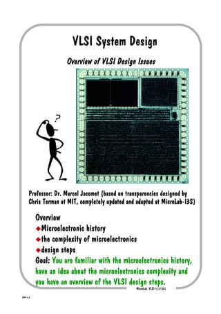
- 1. VLSI System Design Overview of VLSI Design Issues Professor: Dr. Marcel Jacomet (based on transparencies designed by Chris Terman at MIT, completely updated and adapted at MicroLab-I3S) MicroLab- Overview Microelectronic history the complexity of microelectronics design steps Goal: You are familiar with the microelectronics history, have an idea about the microelectronics complexity and you have an overview of the VLSI design steps. MicroLab, VLSI-1 (1/28) JMM v1.4
- 2. What’s expected of you Class/Homework Readings from a Starter Guide to VHDL and some articles. Some 50% in class 50% homework Self- problems to be worked at home. Self- study of the VHDL language with help of the CBT CD from Doulouse. Doulouse. Project Some design exercises to be done in 40% of final grade the lab. Specify, design and simulate a small VHDL design project using a data- data-path / finit state machine. Place & route it on a FPGA target technology (due date: July 19th at 13h00, 2002) Test in- One 70 minute in-class test. Meant 60% of final grade to be duck soup if you’ve been coming to lectures and doing the lab and homework (date: Friday July 12th, 2002). MicroLab, VLSI-1 (2/28) JMM v1.4
- 3. Timetable 4th Semester: Introduction to VLSI System Design Date Topic Self-Study Self- 11- 11-15.3. vlsi1: history & complexity A VLSI tutorial 18- 18-22.3. vlsi8: micro technologies How a silicon int. 25- 25-29.3. -- 11- 11-19.4. vlsi8: micro technologies article Hoff 22-26.4. 22- vlsi21: top-down design, VHDL top- VHDL/CBT 29.4- 29.4-3.5. Ex400, 401 VHDL/CBT 6-10.5. -- VHDL/CBT 13- 13-17.5. vlsi21 & Ex402 VHDL 20- 20-24.5. vlsi21 & Ex404,405 VHDL 27- 27-31.5. Ex406- vlsi21 & Ex406-408 VHDL 3-7.6. vlsi21 & Ex409 chapter 5 10- 10-14.6. vlsi21: & Ex410 VHDL finish 17- 17-21.6. Ex450 project 24- 24-28.6 Ex451 project 1-5.7. Ex452 project 8-12.6. Test project 15- 15-19. 6 test discussion and outlook project 19.6. at 13h00 project due MicroLab, VLSI-1 (3/28) JMM v1.4
- 4. So, what’s VLSI Systems Design all about? bottom- You’ll get a bottom-up tour of how integrated circuits are engineered. We’ll talk about field- field-effect transistors: how they work, how they’re built, effects of new technologies various design and layout techniques, from the ordinary to the bizarre, for creating combinational and sequential circuits, datapaths, memories, datapaths, buffers, regular logic structures, … how you tackle the problem of designing circuits with 1,000,000 gates -- you’re not in Digital Technique anymore! MicroLab, VLSI-1 (4/28) JMM v1.4
- 5. Key Technology Microelectronics microelectronics is a key technology of the world economy technology development is extremely aggressive post- post-grade engineering education is important influence of other technologies like software engineering key technologies may be used as weapons. 1991 Japan hold 80% share of the world production of DRAMs. 4MB DRAMs. Artificial raw material shortage are disastrous. very few Swiss chip fabs. Our raw material is the fabs. high education standard, that means YOU MicroLab, VLSI-1 (5/28) JMM v1.4
- 6. What is a VLSI Circuit? VERY LARGE SCALE INTEGRATED CIRCUIT Technique where many circuit components and the wiring that connects them are manufactured simultaneously into a compact, reliable and inexpensive chip. Early (circa 1977) characterization of circuit “size” before people realized that the number of components per chip was quadrupling every 24 (Moore’s months (Moore’s Law)! This growth rate has slowed in recent years… can you guess why? MicroLab, VLSI-1 (6/28) JMM v1.4
- 7. Course Outline/Brief history Bell Labs lays the groundwork: 1940: Ohl develops PN junction 1945: Shockley’s lab established 1947: Bardeen and Brattain create point- point-contact transistor with two PN junctions. Gain = 18. 1951: Shockley develops junction transistor which can be manufactured in quantity. 1952: Dummer forecasts “solid block [with] layers of insulating, conducting and amplifying materials” 1954: The first transistor radio! Also, TI makes first silicon transistor (price $2.50) MicroLab, VLSI-1 (7/28) JMM v1.4
- 8. Early integration Kilby, Jack Kilby, working at Texas Instruments, first dreamed up the idea of of a monolithic “integrated circuit” in July 1959. By the end of the flip- year, he had constructed several examples, including the flip-flop shown in the patent drawing above. Components are connected by hand- hand-soldered wires and isolated by “shaping” and pn diodes used as resistors. Robert Noyce experimented in the late 40’s with where transistors while a physics major at college. He went to MIT where “much to his surprise, few people had even heard about the transistor.” After getting his PhD in 1953, he worked in industry, industry, finally arriving at Mountain View, CA and Shockley Semiconductor Labs in 1955. MicroLab, VLSI-1 (8/28) JMM v1.4
- 9. “ “ In 1957, Noyce left Shockley’s Semi- lab to form Fairchild Semi- Hoerni. conductor with Jean Hoerni. Gordon Moore is another founder. In early 1958, Hoerni invents technique for diffusing impurities into the silicon to build planar transistors and then using a SiO2 insulator. In mid 1959, Noyce develops first true IC using planar transistors, back-to- back-to-back pn junctions for diode- isolation, diode-isolated silicon resistors and SiO2 insulation with evaporated metal wiring on top. MicroLab, VLSI-1 (9/28) JMM v1.4
- 10. Practice makes perfect... 1.5 mm 1961: TI and Fairchild introduced the first logic IC’s (cost ~$50 in quantity!). This is a dual flip-flop with 4 flip- transistors. 1963: Densities and yields are improving. This circuit has four flip flops. 0.97 mm semi- 1967: Fairchild markets the semi-custom chip shown below. Transistors (organized in columns) could be easily rewired using a two- two-layer interconnect to create different circuits. This circuit contains ~150 logic gates. 3.81 mm 1968: Noyce and Moore leave Fairchild and found Intel. No business plan, just a promise to specialize in memory chips. They raise $3M in two days and move to Santa Clara. By 1971 Intel had 500 employees; by 1983 it had 21,500 employees and $1100M in sales. MicroLab, VLSI-1 (10/28) JMM v1.4
- 11. The Big Bang 2.87 mm In 1970, making good on its promise to its investors Intel starts selling a 1K bit RAM, the 1103. It was a bear to interface to, but its density and cost make it the only game it town. In 1971 Intel introduces the first microprocessor, designed by Ted 4- Hoff. The 4004 had 4-bit buses and a clock rate of 108KHz. It had 2300 transistors and was built in a 10um process. It never captured much interest in the market and was soon eclipsed by its more capable brothers. MicroLab, VLSI-1 (11/28) JMM v1.4
- 12. Exponential Growth Introduced in 1972, the 8008 had 3,500 byte- transistors supporting a byte-wide data path. Despite its limitations, the 8008 was the first microprocessor capable of playing the role of computer CPU as demonstrated on the cover of the July ‘74 issue of Radio-Electronics. Radio- Last, but not least, on our tour is the 8080. Introduced in 1974, the 8080 had 6,000 transistors fab’ed in a 6um process. The clock rate was 2Mhz, more than enough to ignite the personal computer industry. At least Paul Allen and his partner thought so when they wrote a BASIC interpreter for the 8080 in 1975. They would later collaborate in another, more profitable, venture... MicroLab, VLSI-1 (12/28) JMM v1.4
- 13. Today AVP- AVP-III Video Codec from Lucent Technologies art Many disciplines have contributed to the current state of the art in VLSI design: solid- solid-state physics circuit design & layout materials science architecture lithography and fab algorithms device modeling CAD tools We’ll be concentrating on the right-hand column right- MicroLab, VLSI-1 (13/28) JMM v1.4
- 14. “Computer- “Computer- Aided CAD Tools #1 Design” organize generate verify Symbolic layout tools to Standard- Standard-cell place ease the task of physical and route for “random” design; mask verification logic. to ensure manufacturability. Circuit analysis programs predict circuit behavior at all the process corners. Gate-level and behavioral Gate- simulators help you get it right the first time! Tools to do the tedious, repetitive work such as routing,“tiling” a mosaic of building-block cells, or building- verifying that the layout and schematic match. MicroLab, VLSI-1 (14/28) JMM v1.4
- 15. CAD Tools #2 Problem: designing highly complex VLSI circuits (100K to xM fets) fets) classical, iterative procedures are unsuitable precise transistor models are necessary for reliable predictions data inflation Solution: new design methodologies powerful design tools high level design languages silicon compiler would be useful MicroLab, VLSI-1 (15/28) JMM v1.4
- 16. VLSI Design Challenge Goal: designing circuits with increasing complexity in always shorter times computer has to take over routine work deliberate the designer from unnecessary low qualification work shift of design activities to higher level abstract work computer has to support new design methods MicroLab, VLSI-1 (16/28) JMM v1.4
- 17. Chip Complexity #1 Chip classification according to number of active elements and minimal feature size: classification #transistors example SSI 1 - 100 gates MSI 100 - 1k registers LSI 1k - 100k uP VLSI 100K - RAM, sig. proc. ULSI ? year minimal channel length 1970 10µ 10µm 1980 5µm 1985 2µm 1992 0.5µ 0.5µm 2002 2002 0.13 0.13µm 2010 ? MicroLab, VLSI-1 (17/28) JMM v1.4
- 18. Chip Complexity #2 can you really imagine the chip complexity of today's VLSI chips and not just express it as a mere number street map image year feature block chip town 10x10µ 1970 10x10µm 200m 2mm Biel 1980 10x5µm 200m 10x5µ 5mm Paris 10x0.7µ 1992 10x0.7µ 200m 10mm Switzerland MicroLab, VLSI-1 (18/28) JMM v1.4
- 19. Architecture (Multiple choice) This is a picture of (A) a programmable general purpose ASIC with 1/4 million 0.7µ transistors on a 40mm2 designed in a 0.7µm CMOS full custom technology. (B) a processor able to execute 64 knowledge based rules in parallel due to a 3 stage pipelined architecture with hard- hard-coded adder, multiplier, divider architecture. (C) the fastest fuzzy processor in the world, designed MicroLab- by MicroLab-I3S and presented at the international FUZZ‘98 conference in New Orleans ANSWER: _________ MicroLab, VLSI-1 (19/28) JMM v1.4
- 20. Circuit Design & Layout Standard cell Full custom RAM Generator Q: Which engineer drew the most fets? ______ fets? MicroLab, VLSI-1 (20/28) JMM v1.4
- 21. VLSI: The Ideal Implementation Medium? VLSI gives the designer control over almost everything: architecture, logic design, speed, area, power, … densities are increasing, costs decreasing with each passing year is used by almost everyone: “No one gets fired for building an ASIC” was the enabling technology for much of the economic growth of the 80’s and 90’s. It will no doubt continue in its starring role for some time come. Is life really a bowl of cherries? MicroLab, VLSI-1 (21/28) JMM v1.4
- 22. VLSI Fact-of-Life #1: Fact-of- “So much to do, so little time” You need a design methodology : budget ($, speed, area, power, schedule, risk) low- low-level building blocks, high- high-level architecture behavioural design, verification logic design, verification layout, verification MicroLab, VLSI-1 (22/28) JMM v1.4
- 23. VLSI Fact-of-Life #2: Fact-of- “You can’t reach in and fix it” verification” Notice that the word “verification” kept appearing in the previous slide. Mistakes can be costly: find bug(s) ? ? reverify 1 week Ecu 10k new masks 3 days Ecu 25k fab run 12 weeks Ecu 1k/wafer slip ship date Ecu Ecu Ecu There’s a lot that needs checking: circuit must operate at all “corners” verified at building block level logic must be correct, operate reliably verified at RTL/gate level chip has to interoperate with system verified at behavioral level chip has to be manufacturable manufacturable verified at mask level, at tester MicroLab, VLSI-1 (23/28) JMM v1.4
- 24. VLSI Fact-of-Life #3: Fact-of- “Verification is a tedious task” MicroLab, VLSI-1 (24/28) JMM v1.4
- 25. VLSI Fact-of-Life #4: Fact-of- “You can’t find all the bugs” The key word here is “find”: one can’t explore the behaviour of the circuit under all possible conditions some of the bugs arise from unanticipated interactions which, by definition, one never thinks of testing it’s not clear when one is “done” looking for bugs! Time pressures mean that most searches stop too soon. The trick is to choose some implementation rules that result in a circuit that is correct by construction*. For example: choose a simple clocking scheme module inputs must go only to fet gates disallow unclocked feedback make register t(clk-to-Q) > t(hold)+skew t(clk to- clk- use poly only for local interconnect no diffusion wires etc., etc., etc. * or at least avoid as many problems as possible! MicroLab, VLSI-1 (25/28) JMM v1.4
- 26. VLSI Fact-of-Life #5: Fact-of- “Nobody’s perfect” Plan for what happens after you turn it on and nothing happens. provide lot’s of observability and controlability. You’ll need to localize and then find the bug. have a way to run the chip slowly and/or stop it without it burning up or loosing bits. figure out how to track down performance problems without relying on fast I/O (tester pins are slow!) leave room in the budget Ecu) (time, Ecu) for debugging. write and run your manufacturing tests before tape out. MicroLab, VLSI-1 (26/28) JMM v1.4
- 27. Microelectronics in 4th Semester history & microelectronic complexity technologies EXPERIENCE VHDL exercises with data path / fsm CAD tools project synthesis design flow Course material Textbook from Weste & Eshraghian for 4th and 5th semester (voluntary) Copy of transparencies (placeholder for private notes) VHDL Starter (recommended) CAD Exercises on the MicroLab web pages CBT CD on VHDL for your PC (lending from MicroLab in 4th semester) MicroLab, VLSI-1 (27/28) JMM v1.4 different small articles
- 28. Coming Up... top- We’ll be traveling top-down in 4th semester and bottom- bottom-up in 5 & 6 semester: Next topic… Microelectronic technologies like standard cell, gate array, sea-of-gates, macro cell, FPGA, tiny sea-of- micro- micro-controllers. Readings for next time… web CBT tutorials see on http://www.microlab ch/academics/courses microlab. http://www.microlab.ch/academics/courses How a silicon integrated circuit is made (web CBT) A VLSI Tutorial up to chapter with NAND/NOR (web CBT from Uni Manchester) T. Hoff: Article about the µP History (German) (German) erman To learn more about Intel’s early days and to ogle oldie-but- some die photos of oldie-but-goodie chips browse at the Intel link of the MicroLab VLSI course web page. MicroLab, VLSI-1 (28/28) JMM v1.4
- 29. VLSI Design I The MOSFET model Wow ! Are device models as nice as Cindy ? Overview The large signal MOSFET model and second order effects. MOSFET capacitances. Introduction in fet process technology Goal: You can use the large signal equivalent MOS device equation. You are familiar with second order effects like body effect, channel length modulation. You know the MOS capacitances. You know the basic steps in MOS fabrication. MicroLab, VLSI-2 (1/24) JMM v1.4
- 30. Let’s build a MOSFET There are lots of different recipes to choose from. Like most things in life, you get what you pay for: the ability to have good bipolar devices, radiation hardness, reduced latch-up and substrate noise, … latch- are all extra cost options. We’ll consider a general p- process: bulk CMOS with a p-type substrate: 500um slice of a silicon ingot that has been doped with an acceptor (typically boron) to Use <100> surface increase the concentration of holes to 1014/cm3 to minimize surface - 1018/cm3. charge p-type metalliz Back is metallized to provide a good ground connection. Good for n-channel fets, but p-channel n- fets, p- n- fets will need a n-type “well” (or tub) to live in! MicroLab, VLSI-2 (2/24) JMM v1.4
- 31. Next, a “thick” (0.4um) layer of silicon dioxide, called field oxide, is formed on the surface by oxidation in wet oxygen. This is then etched to expose surface where we mosfet: want to make a mosfet: p Now grow a “thin” (0.01um = 100 Å) layer of silicon dioxide, called gate oxide, on the surface by exposing the wafer to dry oxygen. p The gate oxide needs to be of high quality: uniform thickness, no defects! The thinner the gate oxide, the more oomph the fet will have (we’ll see why soon) but the harder it is to make it defect free. MicroLab, VLSI-2 (3/24) JMM v1.4
- 32. On top of the thin oxide a 0.7um thick layer of polycrystalline silicon, called polysilicon or poly for short, is deposited by CVD. The poly layer is patterned and plasma etched (thin ox not covered by poly is etched away too!) exposing the surface where the source and drain junctions will be formed: gate oxide poly wires field oxide (only under poly) exposed surface for source and drain junctions p Poly has a high sheet resistance (25 ohms/square) which can be reduced by adding a layer of a silicided refractory metal such titanium (TiSi2), tantalum (TaSi2) or molybdenum (MoSi2). These have sheet resistances of 1, 3 or 5 ohms per square, respectively. This is great for memory structures that have lots of poly wiring. MicroLab, VLSI-2 (4/24) JMM v1.4
- 33. The entire surface is doped, either by diffusion or ion implantation, with phosphorus (an electron donor) which creates two n-type regions in the substrate. The n- phosphorus also penetrates the poly reducing its resistance and affecting the nfet’s threshold. “self- diffusions are “self-aligned” with poly n+ n+ 20- n+ wires: 20-30 ohms/sq. p Finally an intermediate oxide layer is grown and then reflowed to flatten its surface. Holes are etched in the oxide (where contacts to poly/diff are wanted) and alumin aluminum deposited, patterned and etched. metal wires (0.08 ohms/square) ??? diff contact (0.25 - 10 ohms) n- channel MOS field effect transistor! MicroLab, VLSI-2 (5/24) JMM v1.4
- 34. NFET Operation Picture shows configuration when Vgs < Vto S G D Ids = 0 n+ n+ p mobile holes, mobile electrons, fixed negative ions B fixed positive ions (n+ means heavily depletion layer doped with donors, no mobile carriers, doesn’t imply but fixed negative ions positive charge!) (slight intrusion into n+, but mostly in p area) Terminal with higher G voltage is labelled D, Other symbols: the other is labelled S so Ids >= 0. S D B almost always ground MicroLab, VLSI-2 (6/24) JMM v1.4
- 35. FET = field effect transistor The four terminals of a fet (gate, source, drain and bulk) connect to conducting surfaces that generate a complicated set of electric fields in the channel region which depend on the relative voltages of each terminal. Picture shows configuration when Vgb > Vto gate inversion happens here Eh Ev source drain bulk INVERSION: CONDUCTION: strong A sufficiently strong vertical If a channel exists, a field will attract enough horizontal field will cause electrons to the surface to a drift current from the n- create a conducting n-type channel drain to the source. between the source and drain. Expect Ids proportional to Vds*(W/L)? Vds*(W/L)? MicroLab, VLSI-2 (7/24) JMM v1.4
- 36. Threshold voltage The gate voltage required to form the channel is called the threshold voltage. Many factors affect the gate-source voltage at which the gate- source- channel becomes conductive. Threshold voltage for source-bulk voltage zero: VTO = Vt − ms + Vfb Qb Q ε ox VTO = 2φ F + + φ ms − fc C ox C ox t ox kT N DN A 0.61V for n-channel 2 kT ln N A n- ln 2 -0.61V for p-channel q n i p- q ni 2 ε si q N A 2φ F MicroLab, VLSI-2 (8/24) JMM v1.4
- 37. Body effect (second order) As Vsb increases, the depth of the depletion region increases, exposing more of the fixed acceptor (i.e. negative) ions in the substrate. Thus the second term in the threshold voltage equation on the previous slide increases from 2ε si qN A 2 ΦF to 2ε si qN A (Vsb + 2 ΦF ) n- the threshold voltage of the n-channel transistor is now: 2ε si qN A Vtn = Vtn0 + γ ( Vsb + 2 ΦF − 2 ΦF ) γ= C ox As we’ll see, this effect T2 comes into play in series- series-connected fets Vsb>0 where only one of the T1 fets will have Vsb = 0 and the other fets will Vt2> Vt1 Vsb=0 have Vsb > 0 and a higher threshold voltage. MicroLab, VLSI-2 (9/24) JMM v1.4
- 38. Basic DC equations MOS transistors have 3 regions of operation: (subthreshold subthreshold) cutoff region (subthreshold) linear region (triode region) saturated region (active region) polysilicon gate SiO2 source diffusion drain diffusion W L Cutoff or subthreshold region: <=V Vgs <=Vt Ids = 0 There is still a small current described in the second order effects (weak inversion). Important to model for analog circuits: I ds ∝ Vds MicroLab, VLSI-2 (10/24) JMM v1.4
- 39. “Linear” operating region Vs Vgs > Vt 0 < Vds < Vdsat Ids L Larger Vgs creates Larger Vds increases drift current but deeper channel which also reduces vertical field component increases Ids which in turn makes channel less deep. pinch- Channel will pinch-off, when channel length is mobility Vds = Vgs - Vt = Vdsat almost always min (un > up) allowable fet gain factor k= Cox k=µC 2 W µ ε ox Vds I ds = L t ox ( Vgs − Vt Vds − 2 ) max value at Vds = Vdsat, but then channel is only linear when Vds is small, pinched off (see next slide) otherwise parabolic MicroLab, VLSI-2 (11/24) JMM v1.4
- 40. Saturated operating region Vs Vgs > Vt Vdsat < Vds Ids Voltage at channel end Electrons arriving from source are remains essentially injected into drain depletion region constant at Vdsat so and accelerated towards drain by field drift current also remains proportional to Vds - Vdsat usually constant: device is in reaching the drift velocity limit. saturation. W µ ε ox ( ) 2 I ds (sat ) = Vgs − Vt 2 L t ox this is just Ids from previous slide evaluated at Vds = Vdsat MicroLab, VLSI-2 (12/24) JMM v1.4
- 41. Channel- Channel-length modulation (second order) Vs Vgs > Vt Vdsat < Vds Ids L’ = L - dL dL This looks just like a As Vds increases, fet with a channel length dL get larger of L’ < L. Shorter L’ implies greater Ids... As Vds increases the effective channel length gets shorter so Ids(sat) increases. dL is proportional to Vds − Vdsat but most people approximate channel length modulation as a linear effect: W µ ε ox ( ) (1 + λ V 2 I ds (sat ) = Vgs − Vt ds ) 2 L t ox MicroLab, VLSI-2 (13/24) JMM v1.4
- 42. NFET Ids curves “Put it together and what have you got?” plot of Ids vs. Vds for Vgs = 0 ,1, 2, 3, 4 and 5V Can you find the following in the plot? Ids vs. Vds when Vgs = 0V Ids vs. Vds when Vgs = 5V value of Vt value of Vdsat evidence of body effect evidence of channel length modulation MicroLab, VLSI-2 (14/24) JMM v1.4
- 43. SPICE Models There are different models used in circuit simulators: level 1 is our simple model including the most important second order effects described level 2 model is based on device physics level 3 is a semi-empirical model allowing to match semi- equations to the real circuit: example BSIM model circuit: from Berkeley models subthreshold characteristics summary of the main SPICE DC parameters used in all three models at the end of this chapter . M1 4 3 5 0 nfet W=1u L=0.5u AS=1p AD=1p PS=3u PD=3u . . .MODEL nfet NMOS +TOX=1E- +TOX=1E-8 +CGB0=345p CGS0=138p CGD0=138p +CJ=775u CJSW=344p MJ=0.35 MJSW=0.26 PB=0.75 +. . . . . . MicroLab, VLSI-2 (15/24) JMM v1.4
- 44. MOSFET Capacitance Estimation the dynamic response of MOS systems strongly depends on the parasitic capacitances associated with the MOS device. The total load capacitance on the output of a CMOS gate is the sum of: gate capacitance (of other inputs connected to out) diffusion capacitance (of drain/source regions) routing capacitances (output to other inputs) Cgd drain Cdb gate substrate Cgs Csb source gate Cgb Cgs Cgb Cgd tox channel source drain depletion layer Csb Cdb substrate MicroLab, VLSI-2 (16/24) JMM v1.4
- 45. MOSFET gate capacitances Cg = Cgd + Cgs + Cgb Oxide- Oxide-related capacitances come in two forms: overlap capacitance (extrinsic) since gate slightly overhangs diffusions and bulk: for both Cgs and Cgd amount of overlap C(overlap) = W LD Cox for SPICE for Cgb Cgs = W CGS0 C(overlap) = 2L CGB0 Cgd = W CGD0 Cgb = 2L CGB0 channel- channel-charge related capacitances (intrinsic): cut- cut-off: Cgb = Cox W L Cgs = Cgd = 0 shielded by channel linear: Cgb = 0 Cgs = Cgd = 0.5 Cox W L equally shared between S and D note capacitive coupling of gate and drain/source saturation: Cgb = 0 channel pinched off Cgd = 0 channel shortened Cgs = 0.67 Cox W L MicroLab, VLSI-2 (17/24) JMM v1.4
- 46. MOSFET diffusion capacitances Junction capacitances Cdb and Csb are a function of the applied terminal voltages and diffusion dimensions: source/drain diffusion xj channel sidewall faces bottom junction faces sidewalls face p+ channel p-type substrate channel stop zero- zero-bias C/unit area of bottom junction zero- zero-bias C/unit length of area of diffusion sidewall junction perimeter of diffusion C jA C jsw P C diff = Mj + Mjsw negative for Vj Vj reverse biased 1 − V 1 − V coeff. grading coeff. b b built- built-in junction potential junction voltage coeff. grading coeff. MicroLab, VLSI-2 (18/24) JMM v1.4
- 47. P-channel MOSFETs S G D p+ p+ n p threshold voltage is PFET is built inside its negative since we need B n- own “substrate”: a n-type attract holes to form well or tub diffused into inversion layer p-type bulk substrate. Don’t forget well contacts! Other symbols: G Terminal with lower voltage is labelled D, the other is labelled S S D off: Vgs > Vt B n-well always connected lin: lin: Vgs>Vt, Vds>Vgs-Vt to Vdd to keep pn sat: Vgs>Vt, Vds<Vgs-Vt back- junction back-biased MicroLab, VLSI-2 (19/24) JMM v1.4
- 48. Depletion- Depletion-mode MOSFETs S G D n+ n+ p channel doped with donors B to give negative threshold voltage, i.e., depletion fets are always on. This mosfet is always conducting but, like ordinary enhancement fets, it will conduct more current as Vgs fets, n- increases. One can build logic circuits with only n- channel devices (NMOS): enhancement fets for pulldowns and depletion fets as static pullups. Since NMOS logic pullups. dissipates DC power it’s been largely replaced by CMOS. MicroLab, VLSI-2 (20/24) JMM v1.4
- 49. Coming Up... Next topic… Static characteristics of MOS inverters: input and output voltages, noise margins, power dissipation. Readings for next time… Weste: sections 2 thru 2.23 except 2.2.2.4 - 2.2.2.7 (fet (fet models), 3 thru 3.2.2 (process technology) and 4.3 through 4.3.4 (capacitances) CBT: Study the chip fabrication text of the university of Manchester at the MicroLab VLSI course web link. MicroLab, VLSI-2 (21/24) JMM v1.4
- 50. Useful Constants sym value units description ε0 8.8542E- 8.8542E-12 F/m permittivity εox 3.9 ε0 F/m permittivity of SiO2 εSi 11.7 ε0 F/m permittivity of silicon VT 25.8 mV kT/q (@300°K) kT/q q 1.6022E- 1.6022E-19 C charge of electron k 1.381E- 1.381E-23 J/°K Boltzmann‘s Boltzmann‘s constant ni 1.45E10 cm-3 intrinsic carrier concentration MicroLab, VLSI-2 (22/24) JMM v1.4
- 51. Alcatel 0,5um Process Parameters sym param nmos pmos units description Vt0 VTO 0.61 -0.61 V threshold voltage tox TOX 1E-8 1E-8 m 1E- 1E- thin oxide thickness NA NSUB 4E16 4E16 cm-3 substrate doping density µ U0 290 72 cm2/Vs charge mobility k KP A/V2 fet gain factor γ GAMMA param. V0.5 bulk threshold param. Cox COX capacitance F/m2 oxide capacitance λ α/L V- 1 channel length α modulat.1e- 2e- modulat.1e-8 2e-8 V-1m-1 channel length mod fact. φ0 PB 0.7556 0.78469 V built in junction potent. 2φF PHI 0.77 0.77 V surface inversion pot. Cgb0 CGB0 3.45E- 3.45E-10 dito F/m overlapping cap per 2L Cgs0 CGS0 1.38E- 1.38E-10 dito F/m overlapping cap per W Cgd0 CGD0 1.38E- 1.38E-10 dito F/m overlapping cap per W Cj CJ 7.75E- 8.15E- 7.75E-4 8.15E-4 F/m2 zero-bias cap / unit A zero- Cjsw CJSW 3.44E- 3.54E- 3.44E-10 3.54E-10 F/m zero-bias cap per unit P zero- Mj MJ 0.35 0.36 grading coeff for bottom Mjsw MJSW 0.26 0.27 grading coeff sidewall MicroLab, VLSI-2 (23/24) JMM v1.4
- 52. VLSI- Exercises: VLSI-2 Ex vlsi2.1 (difficulty: easy): Calculate the missing parameters on the previous transparency like intrinsic transconductance k, bulk threshold parameter γ and 0.5µ process) oxide capacitance Cox of an nfet (Alatel 0.5µm process) =100µ =24.9µ Result: kn=100µA/V2, kp=24.9µA/V2, γ=0.334V0.5, =3.45E- Cox=3.45E-7 F/cm2 (see Weste pp48ff) Ex vlsi2.2 (difficulty: easy): Calculate the threshold voltage shift due to the body effect of an nfet at Vsb = 2.2V (Alcatel 0.5µm process) (Alcatel 0.5µ Result: dVtn = 0.282V (see Weste pp55) Ex vlsi2.3 (difficulty: easy): Calculate the 0.5µ transconductance βn of an nfet (Alatel 0.5µm process), W=1 µm, L= 0.5 µm µΑ/ Result: βn=200 µΑ/V2 (see Weste pp53) Ex vlsi2.4 (difficulty: easy): Calculate the capacitances of an nfet with Vsb=Vdb=3V, W=1µm, L=0.5µm, Vsb=Vdb=3V, W=1µ L=0.5µ A=1µ P=3µ (Alatel 0.5µ A=1µm2, P=3µm (Alatel 0.5µm process) Result: Cgate=2.35fF, Cdrain=Csource=1.2fF (see Weste pp183- pp183-191) Weste pp99: 2.10: Have a look at ex 8, 9 MicroLab, VLSI-2 (24/24) JMM v1.4
- 53. VLSI Design I Static characteristics of MOS inverter Static characteristics? Does that mean it’s not going to move? Overview Static transfer characteristic of CMOS gates Goal: You know the transfer characteristic of CMOS gates and know how to calculate noise margins MicroLab, VLSI-3 (1/14) JMM v1.4
- 54. NFET Review D D + G G Vds >= 0 + S - S - Vgs Operating regions: 0.7V cut-off: cut- Vgs < Vt S D linear:V linear: Vgs >= Vt Vds < Vdsat S D Vgs - Vt saturation: Vgs >= Vt Vds >= Vdsat S D Ids Vgs Vds MicroLab, VLSI-3 (2/14) JMM v1.4
- 55. PFET Review D D - G G Vds <= 0 + S - S + Vgs Operating regions: -0.7V cut-off: cut- Vgs > Vt S D linear:V linear: Vgs <= Vt Vds > Vdsat S D Vgs - Vt saturation: Vgs <= Vt Vds <= Vdsat S D -Vds -Vgs -Ids MicroLab, VLSI-3 (3/14) JMM v1.4
- 56. “Bipolar” Logic Isn’t this a CMOS course? Bipolar = two signal levels ‘0’ when V near 0 ‘1’ when V near Vdd Vdd Inverter recipe: pullup: make this connection when Vin near 0 so that Vout = Vdd Vin Vout pulldown: make this connection when Vin near Vdd so that Vout = 0 one power supply => low impedance source for 2 levels receivers have a simple job => only make one decision no DC power if connections not “made” at same time Boolean logic has been around a long time MicroLab, VLSI-3 (4/14) JMM v1.4
- 57. Characterizing Inverters What goals do we want to achieve with our inverter implementation (and, more generally, other functions)? fast propagation delay (next lecture!) low power dissipation compact layout noise immunity Vout voltage- Draw voltage-transfer VOH curve (VTC) for inverter. Shade- Shade-in areas that VTC can’t enter. What can we say about gain? VOL What is “ideal” inv. VTC? Vin VIL VIH MicroLab, VLSI-3 (5/14) JMM v1.4
- 58. Noise Margin Are there other ways of signalling? noise immunity. Since we’re signalling values using voltages, we want good noise margins. This means that we need to make an allowance for noise when assigning voltage levels for valid inputs and outputs definition: NM L = VIL max − VOL max NM H = VOH min − VIH min output input characteristics characteristics Vdd Logical High Output Range VOHmin Logical High Input Range VIHmin VILmax Logical Low Logical Low VOLmax Input Range Output Range Vss MicroLab, VLSI-3 (6/14) JMM v1.4
- 59. Choosing signal voltages This is a subject on which reasonable people can disagree! One possible line of attack: merged VTC for all process corners & Vout devices Step 1: pick VIL and VIH don’t want to amplify noise so find values of Vin where VTC gain = 1 or -1. Choose smallest VIL and largest VIH VIL VIH Vout Step 2: pick VOL and VOH choose values so that VOH (1) VTC is in legal territory (2) leave desired noise margins VOL VIL VIH NML NMH MicroLab, VLSI-3 (7/14) JMM v1.4
- 60. Inverter pulldown devices The NFET makes an ideal pulldown device: Ipd if pullup is off, VOL = ______ no DC connection when Vin < ______ increase width to increase Ipd compact layout saturated pulldown region Vout Vin = Vout Vin = Vout + Vt0 cut- cut-off pulldown region linear pulldown region Vin VIL Vt0 always > Vt0 MicroLab, VLSI-3 (8/14) JMM v1.4
- 61. Inverter pullup devices Resistor. No load on input, VOH=Vdd Will dissipate static power; increasing R will reduce low-to- power and increase noise margin, but low-to-high transition gets slower. Only practical if process undo dop supports undoped poly which has sheet resistance of 10M Ohm/square. Depletion-mode NFET. No load on input, VOH=Vdd. Depletion- Connecting gate to source sets Vgs = 0 so Ipu is determined only by Vout. Layout can be compact since pulldown; pullup is in same well as pulldown; buried contact can be used to connect gate to source. Only found in NMOS processes. Enhancement-mode NFET. VOH= Vdd- Vt unless gate of Enhancement- pullup is driven above Vdd. If gate is not switched off, pullup needs to be weak to avoid excessive power dissipation, but this may entail larger layouts. Useful where PFETs not wanted (e.g., some I/O structures). Pseudo- Pseudo-NMOS using saturated PFET as load fan- device. VOH= Vdd. Useful for building large fan-in NOR gates found in static ROMs and PLAs where static power dissipation is okay. MicroLab, VLSI-3 (9/14) JMM v1.4
- 62. Inverter with PFET pullup Vgs,pu = Vin-Vdd gs, Vds,pu = Vout-Vdd ds, S steady- negligible steady-state G power dissipation Vin D Vout VOL = 0V, VOH = Vdd D VTC transition very sharp switching point can be G S adjusted by fet sizing Vgs,pd = Vin gs, Vds,pd = Vout ds, non- non-vertical only because channel- of channel-length modulation Vout Vin = Vout Vdd n=off lin p= sat sat p= n= p=off lin n= Wn/Wp>1 Wn/Wp>1 Wn/Wp<1 Wn/Wp<1 Vin Vt,p Vt,n Vdd+Vt,p Vdd MicroLab, VLSI-3 (10/14) JMM v1.4
- 63. Build your own VTC In the steady state: Ids,pd(Vin,Vout) = -Ids,pu(Vin-Vdd,Vout-Vdd) ds,pu Ids,pd ds, Ids,pd ds, -Ids,pu ds, Vin = 0.5V -Ids,pu ds, Vin = 1.5V Vout Vout Vout Ids,pd ds, -Ids,pu ds, Vin = 2.5V Vout When both fets are saturated, small changes in Vin produce large changes in Vout Vin Ids,pd ds, Ids,pd ds, -Ids,pu ds, Vin = 3.5V -Ids,pu ds, Vin = 4.5V Vout Vout MicroLab, VLSI-3 (11/14) JMM v1.4
- 64. Ben Bitdiddle’s Buffer! Vin Vout How many would you buy? MicroLab, VLSI-3 (12/14) JMM v1.4
- 65. Coming Up... Next topic… Dynamic characteristics of MOS inverters: propagation delay, effects of rise and fall times. Transistor sizing, interconnect issues, estimating performance. Readings for next time… Weste: Sections 2.3 thrugh 2.3.2 MicroLab, VLSI-3 (13/14) JMM v1.4
- 66. VLSI- Exercises: VLSI-3 Ex vlsi3.1 (difficulty: easy): Calculate the CMOS inverter threshold values for the following confi- confi- 0,5µ gurations (Alcatel 0,5µm process,VDD=3,3V) a) Wn = Ln, Wp = Lp b) Wn = 10 Ln, Wp = Lp c) Wn = Ln, Wp = 10 Lp Result: a) Vinv = 1.30V, b) Vinv = 0.893, c) Vinv = 1.88V (see Weste pp66) Ex vlsi3.2 (difficulty: medium, time consuming): Calculate the noise margin and VIL, VIH, VOL, VOH, for a CMOS inverter operating at 3.3V with βn= βp, Utn= -Utp=0.61V. Result: VIL = 1.39V, VIH = 1.91V, VOL = 0.26V, VOH = 3.04, NML= NML=1.13V Weste pp99: 2.10 ex 5 (difficulty: medium, time consuming): Design an input buffer that may be (V used to interface with a TTL driver (Vdd=3.3V, VOL=0.8V, VOH=2.0V). Show full derivations of =1µ DC conditions. Assume Wn =1µm and Ln = Lp = 0.5µ 0.5µm Result: Wp = 1.51µm 1.51µ MicroLab, VLSI-3 (14/14) JMM v1.4
- 67. VLSI Design I Dynamic characteristics of MOS inverters Wow! 0 to 3.3 volts in 300ps! Overview gate delay modeling power dissipation Goal: You are familiar with CMOS gate delay models like Penfield-Rubenstein and wire models. You Penfield- know the influence of body effect and large loads to gate delay. You know why ground bounce occurres. occurres. You know the different factors in power dissipation. MicroLab, VLSI-4 (1/29) JMM v1.3
- 68. Static properties reviewed sharp transition: inverter good voltage- receiver for voltage- based signalling Vout Ids,n ds,n increasing Wn increasing Wp decreasing Wp decreasing Wn Define theshold voltage Vinv as voltage where Vin = Vout on VTC. Vin VOH=Vdd, VOL=0, sharp transition => good noise margins VOH=Vdd => pfet off when Vin=VOH => no static power VOL=0 => nfet off when Vin=VOL => no static power VTC describes static behaviour. When Vin changes, Vout “lags behind” because it takes time for capacitors to charge/discharge. So, in real, life Vin reaches Vth before Vout does. MicroLab, VLSI-4 (2/29) JMM v1.3
- 69. Choosing what to measure V tf Vin 90% Vin Vout ??? 10% Vout t td tr Rise time, tr = time for a waveform to rise from 10% to steady- 90% of its steady-state value Fall time, tf = time for a waveform to fall from 90% to 10% of its steady-state value steady- Delay time, td = time between input transition (when Vin = ???) and output transition (when Vout = ???). If ??? = Vinv, can delay be negative? does Vinv differ for each gate? so does td(seq. of gates) = sum(td)? should we choose 50% instead of Vinv? MicroLab, VLSI-4 (3/29) JMM v1.3
- 70. Signal delay time Signal delay time is composed as follows gate delay time interconnection delay time due to minimization the delay times decreases the output impedance of buffers increases, thus the importance of interconnection delays increases due to continuing miniaturization, signal delay time becomes less dependent on gate delay but more dependent on interconnection delay time UCC switch level mode of fet switch level mode of inverter Rp Ugs Uds Uin Uout C Cin R Rn MicroLab, VLSI-4 (4/29) JMM v1.3
- 71. Fall time analysis #1 dynamic transition Vout static transition Vin = Vout Vdd n=off lin speed p= sat sat p= n= lin p=off n= Vin Vt,p Vt,n Vdd+Vt,p Vdd the switching speed is limited by the time taken to discharge the capacitance CL the static transition curve moves to the right if the input transition is fast cut- p-fet gets cut-off during the whole falling output time n-fet immediately gets saturated, later on linear MicroLab, VLSI-4 (5/29) JMM v1.3
- 72. Fall time analysis #2 Saturated: Vout >= Vdd - Vt,n dVout βn = − (Vdd − Vt,n ) 2 CL Vout dt 2 So, time to fall from 0.9Vdd to Idsat,n dsat,n CL Vdd - Vt,n is given by 2C L 0.9V dd β n (Vdd − Vt,n ) 2 ∫Vdd − Vt, n dVout Linear: Vout < Vdd - Vt,n dVout Vout CL =− = −Idn function Vout dt Rn of Vout Rn CL So, time to fall from Vdd - Vt,n to 0.1Vdd is given by Vdd −Vt ,n dVout CL ∫ 0.1Vdd I dn Adding to get total fall time (Weste, Eq 4.37): Vt,n/Vdd CL 2 (n − 0.1 ) tf = + 0.5 ln (19 − 20n ) β n Vdd (1 − n ) (1 - n ) tr is similar equals 3 to 4 for Vdd=3V-5V and Vt,n=.5V-1V =3V- =.5V- equals 3.6 for C05M MicroLab, VLSI-4 (6/29) JMM v1.3
- 73. Estimating delays In most CMOS circuits, the delay of a single gate is dominated by the output raise and fall time. Thus: tr tf t dr = t df = 2 2 Having found a general form for approximate rise and fall times, one might estimate all delays using the same general form: L width expressed t delay = A delay CL W as multiple of minimum width looks like a resistor! Where Adelay is a constant that depends on the power supply and transition voltages, the process and the minimum mosfet dimensions. This last dependency might strike one as odd, but usually all mosfets are built using the minimum allowable mosfet length for the process. Rather than solve the equations analytically, one can use Spice to determine the value of various useful constants: Ar, Af, Adr, Adf. These can be used in quick&dirty calculations for sizing transistors during the design process. MicroLab, VLSI-4 (7/29) JMM v1.3
- 74. Input rise/fall & delay How do input rise and fall times affect delay? fast inputs will quickly turn off one mosfet and provide maximum Vgs to the driving mosfet for most of the output transition slow inputs will leave both mosfets on longer, reducing effective current to/from load capacitance and Vgs will be lower than above. So we might expect slower input transitions to lead to longer output delay times. One rule of thumb (Weste, p. 216ff) Weste, (Weste ~0.2 for Vtn = 0.61V, Vdd = 3.3V 1 + 2n t dr = t dr −step + t f,in 6 1 − 2p t df = t df −step + t r,in 6 valid for input transitions that aren’t “too” long MicroLab, VLSI-4 (8/29) JMM v1.3
- 75. Bootstrapping & delay CGD When the input starts to rise, the output, which was high, starts to fall. Thus the voltage across CGD changes requiring the input to supply more current to charge CGD, slowing the input transition. Since CGD is small, this is usually a small effect. When inverter is biased into its linear region, CGD may appear multiplied by the gain of the inverter (Miller effect). This doesn’t usually matter in digital circuits since the input passes rapidly through linear region. Useful in analog circuits... MicroLab, VLSI-4 (9/29) JMM v1.3
- 76. Multiple inputs & delay Cout A Cab B Intermediate Cbc node C capacitances Ccd D How should we model delays when we have multiple inputs? When A, B, C and D are logic 1: treat series mosfets as resistances in series. Lump intermediate node capacitance with load capacitance. t d = ∑iR i ∑ iC i use Penfield-Rubenstein model which predicts Penfield- t d = ∑iR i C i where Ri is the summed resistance from point i to ground and Ci is the capacitance at point i. Penfield- Penfield-Rubenstein Slope Model uses effective resistance simulated by Spice: t df Rn = MicroLab, VLSI-4 (10/29) C JMM v1.3
- 77. Body effect & delay A B C D If A goes from 0 to 1 while B, C and D are 1, then all the intermediate nodes in the pulldown chain have already been discharged and the top mosfet sees only a small body effect. If D goes from 0 to 1 while A, B and C are 1, then the intermediate nodes are all one Vt below Vdd and the upper mosfets see a larger body effect. Thus A is the “faster” input! MicroLab, VLSI-4 (11/29) JMM v1.3
- 78. Driving large loads #1 If large loads have to be driven, the delay may increase drastically. Large loads are output capacitances, clock trees, etc. C t d = t inv L = 1000 ⋅ t inv 1 CG CG CL=1000 CG A possibility to reduce the delay, but probably not the optimum: 40 ⋅ t inv 5 ⋅ t inv 5 ⋅ t inv 1 40 200 CG CL=1000 CG 40 200 1000 td = ⋅ t inv + ⋅ t inv + ⋅ t inv = 50 ⋅ t inv 1 40 200 MicroLab, VLSI-4 (12/29) JMM v1.3
- 79. Driving large loads #2 To drive a large load capacitance one might employ a sequence of n inverters, each a factor “a” larger than the previous one: 1 a a2 a3 CG CL n=4 inverters The delay through each stage is atd where td is the average delay of a minimum-sized inverter driving another minimum- minimum- minimum- sized inverter. We want an = (CL/CG), so CL a t d Total delay = n (a t d ) = ln C G ln (a ) Thus, total delay is minimized when a = e = 2.7 7 6 5 4 in practice 3 a=3...5 2 1 0 0 1 2 3 4 5 6 7 8 MicroLab, VLSI-4 (13/29) JMM v1.3
- 80. Power dissipation #1 the power consumption is low compared to other technologies scaling down increases the power dissipation density with respect to chip area power dissipation produces heat on the chip, which has to be carried off through the chip socket power dissipation is one of the limiting factors in todays CMOS VLSI chips low power applications is a speciality of EM Neuenburg, (Neuenburg, watches, battery applications, etc) MicroLab, VLSI-4 (14/29) JMM v1.3
- 81. Power dissipation #2 sources of power dissipation: static power dissipation (quiescent current) dynamic power dissipation dc power dissipation: short circuit current (power to dissipat ground) due to switching re- ac power dissipation: capacitor current (charging, re- charging) due to switching static power dissipation there is always one fet off, so only leakage current is present I0 = I S (e qV / kT − 1 ) PS = ∑ I0 ⋅ VDD MicroLab, VLSI-4 (15/29) JMM v1.3
- 82. Dynamic power dissipation #1 Comparison of dynamic short circuit current vs. capacitive current. As expected, the short circuit current have a less important contribution when the load gets large. Slower input transition would increase short circuit current. Uin Uout W/L=4 Idsn Uin Uout-A out- W/L=2 Idsp W/L=4 Idsn Uin Uout-B out- W/L=2 Idsp 50fF W/L=4 Idsn Uin Uout-C out- Idsp W/L=2 200fF MicroLab, VLSI-4 (16/29) JMM v1.3
- 83. Dynamic power dissipation #2 square- Average dynamic power for switching a square-wave input 1/t with a repetition frequency of fp = 1/tp is (capacitor current) t p /2 tp 1 1 Pd = ∫ in (t )Vout dt + ∫ i p (t )(VDD − Vout )dt tp 0 t p t p /2 dt, Assuming a step input and taking in(t) = CLdVout/dt, i.e., the capacitive current, we get: Vdd 0 CL CL Pd = tp ∫ Vout dVout + t p 0 ∫ (V Vdd DD − Vout )d (VDD − Vout ) Aha! Now one can see why everybody changes from 5V to 3.3V and to 2.5V! 2 C L VDD 2 Pd = = C L VDD fp tp proportional to switching frequency but independent of device parameters MicroLab, VLSI-4 (17/29) JMM v1.3
- 84. Dynamic power dissipation #3 Short circuit power dissipation is given by Psc = Imean ⋅ VDD tr tf VDD+Vtp Vtn tp Imax Imean t1 t2 t3 The above waveform shows the short circuit current β t rf ⋅ (VDD − 2 Vt ) 3 Psc = 12 t p MicroLab, VLSI-4 (18/29) JMM v1.3
- 85. Total power dissipation Total power dissipation is: Ptotal = Ps + Pd + Psc dynamic power dissipation is dominant use switching activity to estimate power dissipation: 2 Pd = n switching ⋅ C total ⋅ VDD ⋅ f switching activity: nswitching = percentage of switching gates there exist simulators estimating power dissipation using the switching activity MicroLab, VLSI-4 (19/29) JMM v1.3
- 86. Build your own power meter current- linear current-controlled current source + Vs = 0 Is g*I g*Is RY CY Vy - Vy(0) = 0V Device or Periodic input Circuit CL Vin(t) = Vin(t+T) If one chooses Vdd C y g= T and RyCy >> T Then Vy(T) in volts will equal the average dynamic power in watts drawn from the power supply over one period. MicroLab, VLSI-4 (20/29) JMM v1.3
- 87. Power and ground bounce power- Metal power-carrying conductors have to be sized for three reasons: metal migration power supply noise RC delay general rule: limit current density J AL ≈ 0.4... 1mA / µm contact replication I I I I MicroLab, VLSI-4 (21/29) JMM v1.3
- 88. “It’s the wires, stupid” As process dimensions shrink, wiring capacitances start to dominate the mosfet capacitances. To estimate wiring capacitances, consider the following figure: l w t h Cpp fringing- fringing-field parallel-plate parallel- capacitance capacitance Parallel- Parallel-plate capacitance given in process files. Fringing capacitance is significant when t is comparable to h. MicroLab, VLSI-4 (22/29) JMM v1.3
- 89. Fringing Capacitance Figure 6.11 from CMOS Digital Integrated Circuits: Analysis and Design, by Kang and Leblebici: Leblebici: For a long conductor where (t/h)=0.4, (w/h)=0.25, (w/l)=0, the total capacitance may be 10x the parallel plate capacitance. MicroLab, VLSI-4 (23/29) JMM v1.3
- 90. Wire model? Today, the longest wire on a VLSI chip might be 2cm which has “time of flight” of ~130ps assuming εSiO2 = 3.9 ε0 If the signal rise/fall time is longer than the time of flight we can model wires as a distributed RC network. Longer wires or shorter rise/fall times require the wire to be modelled as a transmission line. For short wires, a lumped RC model is sufficient. For longer wires, we use the distributed RC model where signal propagation can be shown to obey the diffusion equation: R/unit length dV d 2 V rc = 2 dt dx C/unit length distance from driver Which means the prop time tx = kx2 with the signal “edge” becoming dispersed with increasing x. MicroLab, VLSI-4 (24/29) JMM v1.3