Characterization of the Wireless Channel

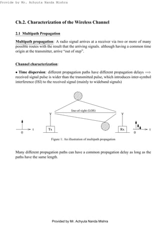
Ch.2. Characterization of the Wireless Channel
2.1 Multipath Propagation
Multipath propagation: A radio signal arrives at a receiver via two or more of many
possible routes with the result that the arriving signals. although having a common time
origin at the transmitter, arrive “out of step”.
Channel characterization:
• Time dispersion: different propagation paths have different propagation delays =⇒
received signal pulse is wider than the transmitted pulse, which introduces inter-symbol
interference (ISI) to the received signal (mainly to wideband signals)
Tx
0
t
00
0000
00
11
1111
11
000000000
000
111111111
111
line-of-sight (LOS)
Rx t
0
Figure 1: An illustration of multipath propagation
Many different propagation paths can have a common propagation delay as long as the
paths have the same length.
Provide by Mr. Achyuta Nanda Mishra
Provided by Mr. Achyuta Nanda Mishra

Wireless Communications and Networking Ch2 - Page 2 of 44
All the scatterers located on an ellipse with the transmitter and receiver as the foci cor-
responds to a distinct propagation delay, and is therefore called a distinct scatterer.
Copyright Prentice Hall
Scatterer
RxTx
Figure 2: Ellipsoidal portrayal of scatterer location
The receiver cannot distinguish the individual received signal component coming from
path 1 from the component coming from path 2, etc.
=⇒ The received signal component with propagation delay τ1 = d/c (where c is the
velocity of light) is a result of the multiple propagation paths.
• Fading: Consider transmitting a single-tone sinusoid. For simplicity, consider a two-
path channel, where the delay of the line-of-sight (LOS) or direct path is assumed to be
zero, and the delay of the non-line-of-sight (NLOS) or reﬂected path is τ.

0
0
0
00
0
0
1
1
1
11
1
1
0
0
0
00
0
0
1
1
1
11
1
10101
0101
0
0
1
1
0
0
1
101
0
0
1
1
0
0
1
10101
0000000000000000000000
0000000000000000000000
1111111111111111111111
1111111111111111111111
Transmitter
Receiver
c Prentice Hall
α1 cos(2πfct)
α2 cos(2πfc(t − τ))
Figure 3: A channel with two propagation paths
The received signal, in the absence of noise, can be represented as
r(t) = α1 cos(2πfct) + α2 cos(2πfc(t − τ)), (1)
where α1 and α2 are the amplitudes of the signal components from the two paths respec-
tively. The received signal can also be represented as
r(t) = α cos(2πfct + φ), (2)
where
α = α2
1 + α2
2 + 2α1α2 cos(2πfcτ)
and
φ = − tan−1
[
α2 sin(2πfcτ)
α1 + α2 cos(2πfcτ)
]
are the amplitude and phase of the received signal. Both α and φ are functions of α1, α2,
and τ.

0 0.5 1 1.5 2 2.5
0
0.5
1
1.5
2
2.5
3
3.5
4
fc
τ
α1
+α2
α1
−α2
© Prentice Hall
Thereceivedsignalamplitudeα
Figure 4: The amplitude ﬂuctuation of the two-path channel with α1 = 2 and α2 = 1
As the mobile user and/or scatterer moves, fcτ changes → the two received components
add constructively (when fcτ = 0, 1, 2, . . .) or destructively (when fcτ = 0.5, 1.5, 2.5, . . .).
=⇒ |r(t)| is a function of t, referred to as amplitude fading.
At each deep fade, instantaneous SNR ↓ −→ BER ↑.
In summary, multipath propagation in the wireless mobile environment results in a
fading dispersive channel.

2.2 The Linear Time-Variant Channel Model
Consider a multipath propagation environment with N distinct scatterers, each charac-
terized by amplitude ﬂuctuation αn(t) and propagation delay τn(t) , n = 1, 2, . . . , N.
Consider a narrowband signal ˜x(t) transmitted over the wireless channel at a carrier
frequency fc, such that
˜x(t) = ℜ{x(t)ej2πfct
}, (3)
where x(t) is the complex envelope of the signal.
In the absence of background noise, the received signal at the channel output is
˜r(t) = ℜ{
N
n=1
αn(t)x(t − τn(t))ej2πfc(t−τn(t))
}
= ℜ{r(t)ej2πfct
},
where r(t) is the complex envelope of the received signal and can be represented as
r(t) =
N
n=1
αn(t)e−j2πfcτn(t)
x(t − τn(t)). (4)
As the mobile user moves, αn(t) and τn(t) are a function of t =⇒ the channel is linear
time-variant.
=⇒ The channel impulse response depends on the instant that the impulse is applied to
the channel.

Channel impulse response
Linear time-invariant (LTI) channel:
0
0
0 0LTI channel
c Prentice Hall
δ(t)
δ(t − t1)
t1
r(t) = h(t)
r(t) = h(t − t1)
h(t)
x(t) r(t)
t
t
t
t
Figure 5: The linear time-invariant channel model
We can use h(t) to describe the channel, where t is a variable describing propagation
delay, assuming that the impulse is always applied to the channel at time zero.
Linear time-variant (LTV) channel:
0
0
LTV channel 00
c Prentice Hall
δ(t)
δ(t − t1)
t1
x(t) r(t)
h(τ, t)
r(t) = h1(t)
r(t) = h2(t) = h1(t − t1)
t
t
t
t
Figure 6: The linear time-variant channel model
The channel impulse response is a function of two variables: one describing when the
impulse is applied to the channel, the other describing the moment of observing the
channel output or the associated propagation delay.

Definition:
The impulse response of an LTV channel, h(τ, t), is the channel output at t in
response to an impulse applied to the channel at t − τ.
The received signal is
r(t) =
∞
−∞
h(τ, t)x(t − τ)dτ. (5)
The channel impulse response for the channel with N distinct scatterers is then
h(τ, t) =
N
n=1
αn(t)e−jθn(t)
δ(τ − τn(t)), (6)
where θn(t) = 2πfcτn(t) represents the carrier phase distortion introduced by the nth
scatterer.
Note:
τn(t) changes by 1/fc −→ θn(t) changes by 2π
=⇒ a small change in the propagation delay −→ a small change in αn(t) and τn(t), but
a significant change in θn(t)
That is, the carrier phase distortion θn(t) is much more sensitive to user mobility than
the amplitude fluctuation αn(t).

Time-variant transfer function
Linear time-invariant channel:
H(f) = F[h(t)] (7)
The channel output in the frequency domain is
R(f) = H(f)X(f). (8)
Linear time-variant channel:
Deﬁnition
The time-variant transfer function of an LTV channel is the Fourier transform
of the impulse response, h(τ, t), with respect to the delay variable τ.



H(f, t) = Fτ [h(τ, t)] =
∞
−∞ h(τ, t)e−j2πfτ
dτ
h(τ, t) = F−1
f [H(f, t)] =
∞
−∞ H(f, t)e+j2πfτ
df
where the time variable t can be viewed as a parameter.

r(t) =
∞
−∞
h(τ, t)x(t − τ)dτ
=
∞
−∞
x(t − τ)[
∞
−∞
H(f, t) exp(j2πfτ)df]dτ
=
∞
−∞
H(f, t){
∞
−∞
x(t − τ) exp[−j2πf(t − τ)]dτ} exp(j2πft)df
=
∞
−∞
H(f, t)[
−∞
∞
x(ξ) exp(−j2πfξ)(−dξ)] exp(j2πft)df
=
∞
−∞
H(f, t)X(f) exp(j2πft)df
△
=
∞
−∞
R(f, t) exp(j2πft)df
where
R(f, t) = H(f, t)X(f)
and
X(f) = F[x(t)].

Summary:
c Prentice Hall
x(t) r(t)
R(f, t) = H(f, t)X(f)X(f)
h(τ, t)
Fτ
−→
←−
F−1
f
H(f, t)
Figure 7: Frequency-time channel representation
where
r(t) =
∞
−∞
R(f, t) = H(f, t)X(f)
X(f) =
∞
−∞
x(t) exp(−j2πft)dt
r(t) =
∞
−∞
R(f, t) exp(j2πft)df.

Example 2.1:
Consider an LTV channel with the impulse response given by
h(τ, t) = 4 exp(−τ/T) cos(Ωt), τ ≥ 0,
where T = 0.1 ms and Ω = 10π.
a. Find the channel time-variant transfer function H(f, t).
b. Given that the transmitted signal is
x1(t) =
1, |t| ≤ T0
0, |t| > T0
,
where T0 = 0.025 ms, ﬁnd the received signal in the absence of background noise.
c. Repeat part (b) if the transmitted signal is
x2(t) = x1(t − T1),
where T1 = 0.05 ms.
d. What do you observe from the results of parts (b) and (c)?
Solution:
a. The time-variant transfer function is
H(f, t) = Fτ [h(τ, t)]
= Fτ [4 exp(−τ/T) cos(Ωt)]
= 4 cos(Ωt)Fτ [exp(−τ/T)]
=
4T cos(Ωt)
1 + j2πfT
.
b. The received signal is calculated as follows:
r1(t) =
+∞
−∞
h(τ, t)x1(t − τ)dτ
=
∞
0
4 exp(−τ/T) cos(Ωt)x1(t − τ)dτ
=



0, t ≤ −T0
4T cos(Ωt)[1 − exp(−t+T0
T )], −T0 < t < T0
4T cos(Ωt)[exp(−t−T0
T ) − exp(−t+T0
T )], t ≥ T0

−0.1 −0.05 0 0.05 0.1 0.15 0.2 0.25 0.3 0.35 0.4
−1.5
−1
−0.5
0
0.5
1
1.5
t (ms)
x
1
(t)andr
1
(t)/T
© Prentice Hall
x
1
(t)
r
1
(t) / T
(a)
0 0.1 0.2 0.3 0.4 0.5
−1.5
−1
−0.5
0
0.5
1
1.5
t (ms)
x
2
(t)andr
2
(t)/T
© Prentice Hall
x
2
(t)
r
2
(t) / T
(b)
Figure 8: The transmitted signals xi(t) and normalized received signals ri(t)/T (i = 1 and 2) in Example
2.1

The transmitted and received signals are plotted in Figure 8(a).
c. Similar to part (b), the received signal is calculated as follows:
r2(t) =
+∞
−∞
h(τ, t)x2(t − τ)dτ
=
∞
0
4 exp(−τ/T) cos(Ωt)x1(t − T1 − τ)dτ
=



0, t ≤ T1 − T0
4T cos(Ωt)[1 − exp(−t−T1+T0
T )], T1 − T0 < t < T1 + T0
4T cos(Ωt)[exp(−t−T1−T0
T ) − exp(−t−T1+T0
T )], t ≥ T1 + T0
The transmitted and received signals are plotted in Figure 8(b).
d. From Figure 8, it is observed that: (1) the received signals have a larger pulse width
than the corresponding transmitted signals because the channel is time dispersive;
and (2) even though the transmitted signal x2(t) is x1(t) delayed by T1, the received
signal r2(t) is not r1(t) delayed by T1 because the channel is time varying.

2.3 Channel Correlation Functions
Assumptions:
(a) the channel impulse response h(τ, t) is a wide-sense stationary (WSS) process;
(b) the channel impulse responses at τ1 and τ2, h(τ1, t) and h(τ2, t), are uncorrelated if
τ1 = τ2 for any t.
→ wide-sense stationary uncorrelated scattering (WSSUS) channel
Delay power spectral density (psd)
The autocorrelation function of h(τ, t) is
φh(τ1, τ2, ∆t)
△
=
1
2
E[h∗
(τ1, t)h(τ2, t + ∆t)]
= φh(τ1, ∆t)δ(τ1 − τ2)
or equivalently,
φh(τ, τ + ∆τ, ∆t) = φh(τ, ∆t)δ(∆τ), (9)
where
φh(τ, ∆t) = φh(τ, τ + ∆τ, ∆t)d∆τ.
At ∆t = 0, we deﬁne
φh(τ)
△
= φh(τ, 0). (10)
From Eqs. (9) – (10), we have
φh(τ) = F∆τ [φh(τ, τ + ∆τ, ∆t)]|∆t=0
= F∆τ {
1
2
E[h∗
(τ, t)h(τ + ∆τ, t)]}.

φh(τ) measures the average psd at the channel output as a function of the propagation
delay, τ, and is therefore called the delay psd of the channel, also known as the multipath
intensity proﬁle. The nominal width of the delay psd pulse is called the multipath delay
spread, denoted by Tm.
0 c Prentice Hall
φh(τ)
Tm
τ
Figure 9: Delay power spectral density
The nth moment of the delays
¯τn =
τn
φh(τ)dτ
φh(τ)dτ
. (11)
The mean propagation delay, or ﬁrst moment, denoted by ¯τ, is
¯τ =
τφh(τ)dτ
φh(τ)dτ
(12)
and the rms (root-mean-square) delay spread, denoted by στ , is
στ =
(τ − ¯τ)2
φh(τ)dτ
φh(τ)dτ
1/2
. (13)
In calculating a value for the multipath delay spread, it is usually assumed that
Tm ≈ στ .

Frequency and Time Correlation Functions
The autocorrelation function of H(f, t)is
φH(f1, f2, t, ∆t)
△
=
1
2
E[H∗
(f1, t)H(f2, t + ∆t)]
WSS
=⇒ φH(f1, f2, ∆t) =
1
2
E[H∗
(f1, t)H(f2, t + ∆t)]
US
=⇒ φH(f1, f2, ∆t) =
1
2
E{[ h(τ1, t)e−j2πf1τ1
dτ1]∗
[ h(τ2, t + ∆t)e−j2πf2τ2
dτ2]}
=
1
2
E[h∗
(τ1, t)h(τ2, t + ∆t)]e−j2π(f2τ2−f1τ1)
dτ1dτ2
WSS
= φh(τ1, τ2, ∆t)e−j2π(f2τ2−f1τ1)
dτ1dτ2
US
= φh(τ1, ∆t)δ(τ1 − τ2)e−j2π(f2τ2−f1τ1)
dτ1dτ2
= φh(τ1, ∆t)e−j2π(f2−f1)τ1
dτ1
= φh(τ, ∆t)e−j2π(∆f)τ
dτ (∆f = f2 − f1)
△
= φH(∆f, ∆t) — time-frequency correlation function.
Frequency correlation function:
Let ∆t = 0, we have
φH(∆f)
△
=
1
2
E[H∗
(f, t)H(f + ∆f, t)]
= φh(τ)e−j2π∆fτ
dτ.

Note:
• φh(τ) and φH(∆f) is a pair of Fourier transform.
• uncorrelated scattering =⇒WSS H(f, t) w.r.t. f
• φH(∆f) characterizes the correlation of channel gains at f and f + ∆f for any t.
0
c Prentice Hall(∆f)c
∆f
|φH(∆f)|
Figure 10: Frequency-correlation function and channel coherence bandwidth
φH(∆f) provides a measure of the “frequency coherence” of the channel.
• coherence bandwidth: recall the channel with 2 propagation paths
0
00
0
00
0
1
11
1
11
1
0
00
0
00
0
1
11
1
11
10
0
1
1
0
0
1
1
0101
0
0
1
1
0
0
1
10101
00
0
11
1
00
0
11
1
0101
0000000000000000000000
0000000000000000000000
1111111111111111111111
1111111111111111111111
Transmitter
Receiver
c Prentice Hall
α1 cos(2πfct)
α2 cos(2πfc(t − τ))
Figure 11: A channel with two propagation paths
The effect of the 2-path channel on the received signal depends on the signal fre-
quency. With the same τ, two signals A cos(2πf1t) and A cos(2πf2t) will be affect
differently.

0 0.5 1 1.5 2 2.5
0
0.5
1
1.5
2
2.5
3
3.5
4
fc
τ
α1
+α2
α1
−α2
© Prentice Hall
Thereceivedsignalamplitudeα
Figure 12: The amplitude ﬂuctuation of the two-path channel with α1 = 2 and α2 = 1
=⇒ |f1 − f2| ↑ =⇒ |r1(t)| and |r2(t)| at any t will be uncorrelated.
Deﬁnition: The maximum frequency difference for which the signals are still strongly
correlated is called the coherence bandwidth of the channel, denoted by (∆f)c.
=⇒ Two sinusoids with frequency separation larger than (∆f)c are affected differ-
ently by the channel at any t.

• Let Ws denote the bandwidth of the transmitted signal.
If (∆f)c < Ws, the channel is said to exhibit frequency selective fading which
introduces severe ISI to the received signal;
If (∆f)c ≫ Ws, the channel is said to exhibit frequency nonselective fading or
ﬂat fading which introduces negligible ISI.
• φh(τ) ↔ φH(∆f) =⇒ (∆f)c ≈ 1/Tm.

Time correlation function φH(∆t):
Letting ∆f = 0 in the time-frequency correlation function φH(∆f, ∆t), we have
φH(∆t)
△
= φH(0, ∆t) =
1
2
E[H∗
(f, t)H(f, t + ∆t)]. (14)
• φH(∆t) characterizes, on average, how fast the channel transfer function changes
with time at each frequency.
• The nominal width of φH(∆t), (∆t)c, is called the coherence time of the fading
channel.
• If the channel coherence time is much larger than the symbol interval of the trans-
mitted signal, the channel exhibits slow fading.
• φH(∆t) is independent of f due to the US assumption =⇒ US in the time domain
is equivalent to WSS in the frequency domain.
0
c Prentice Hall
(∆t)c
∆t
|φH(∆t)|
Figure 13: Time-correlation function and channel coherence time

Doppler Power Spectral Density
Doppler shifts:
An LTV channel introduces Doppler frequency shifts: Given the transmitted signal fre-
quency fc, the received signal frequency is fc+ν(t), where ν(t) is the Doppler frequency
shift and is given by
ν(t) =
V fc
c
cos θ(t).
0
0
0
00
1
1
1
110
0
1
1
00
00
11
11
0
0
1
1
00110011
00
00
11
11
00
00
11
11
0011001100110101
010
0
0
00
1
1
1
11
c Prentice Hall
θ(t)
VMS
BS
x
Figure 14: The Doppler effect
Consider the wireless channel with N distinct scatterers where the propagation delay can
be approximated by its mean value ¯τ.
h(τ, t) ≈
N
n=1
αn(t) exp[−j2πfcτn(t)]δ(t − ¯τ)
△
= Z(t)δ(τ − ¯τ), (15)
r(t) =
+∞
−∞
=
+∞
−∞
[Z(t)δ(τ − ¯τ)]x(t − τ)dτ
= Z(t)x(t − ¯τ).
In the frequency domain, the received signal is
R(f) = F[r(t)]
= F[Z(t)x(t − ¯τ)]
= F[Z(t)] ⋆ F[x(t − ¯τ)]
= F[Z(t)] ⋆ [X(f)e−j2πf ¯τ
],

=⇒ The channel indeed broadens the transmitted signal spectrum by introducing new
frequency components, a phenomenon referred to as frequency dispersion.
Doppler-spread function H(f, ν):
H(f, ν) is the channel gain associated with Doppler shift ν to the input signal component
at frequency f.
R(f) =
+∞
−∞
X(f − ν)H(f − ν, ν)dν. (16)
Relation between H(f, t) and H(f, ν):



H(f, ν) = Ft[H(f, t)] =
+∞
−∞ H(f, t)e−j2πvt
dt
H(f, t) = F−1
ν [H(f, ν)] =
+∞
−∞ H(f, ν)e+j2πνt
dν
=⇒ being time-variant in the time domain can be equivalently described by having
Doppler shifts in the frequency domain.

Autocorrelation function of H(f, ν):
ΦH(f1, f2, ν1, ν2)
△
=
1
2
E[H∗
(f1, ν1)H(f2, ν2)
=
1
2
E[H∗
(f1, t1)H(f2, t2)]ej2πν1t1
e−j2πν2t2
dt1dt2
WSSUS
= φH(∆f, ∆t)e−j2π[ν2(t1+∆t)−ν1t1]
d∆tdt1
(where ∆f = f2 − f1 and ∆t = t2 − t1)
= φH(∆f, ∆t)e−j2πν2∆t
d∆t e−j2π(ν2−ν1)t1
dt1
= ΦH(∆f, ν2)δ(ν2 − ν1)
where
ΦH(∆f, ν) = φH(∆f, ∆t)e−j2πν∆t
d∆t
is the Fourier transform of φH(∆f, ∆t) w.r.t. ∆t.
At ∆f = 0,
ΦH(ν)
△
= ΦH(0, ν) =
∞
−∞
φH(∆t)e−j2πν∆t
d∆t.
• ΦH(ν) is the Fourier transform of the channel correlation function φH(∆t).
=⇒ ΦH(ν) is psd as a function of the Doppler shift ν.
=⇒ ΦH(ν) is called Doppler power spectral density function.
0
c Prentice Hall
Bd
ν
ΦH(ν)
Figure 15: Doppler power spectral density and Doppler spread

• The nominal width of the Doppler psd, Bd, is called the Doppler spread.
• Since φH(∆t) ↔ ΦH(ν),
(∆t)c ≈
1
Bd
.
• The mean Doppler shift is
¯ν =
νΦH(ν)dν
ΦH(ν)dν
and the rms Doppler spread is
σν = [
(ν − ¯ν)2
ΦH(ν)dν
ΦH(ν)dν
]1/2
.
As an approximation, it is usually assumed that
Bd ≈ σν.

Example 2.3 Delay psd and frequency-correlation function
Consider a WSSUS channel whose time-variant impulse response is given by
h(τ, t) = exp(−τ/T)n(τ) cos(Ωt + Θ), τ ≥ 0,
where T and Ω are constants, Θ is a random variable uniformly distributed in [−π, +π],
and n(τ) is a random process independent of Θ, with E[n(τ)] = µn and E[n(τ1)n(τ2)] =
δ(τ1 − τ2).
a. Calculate the delay psd and the multipath delay spread.
b. Calculate the frequency correlation function and the channel coherence bandwidth.
c. Determine whether the channel exhibits frequency-selective fading for GSM sys-
tems with T = 0.1 ms.
Solution:
a. From Eq. (11), we have
φh(τ) = F∆τ {
1
2
E[h∗
(τ, t)h(τ + ∆τ, t]}
= F∆τ {
1
2
E[n(τ)n(τ + ∆τ)]E[e−(2τ+∆τ)/T
cos2
(Ωt + Θ)]}, τ ≥ 0
= F∆τ {
1
4
e−(2τ+∆τ)/T
δ(∆τ)E[1 + cos(2Ωt + 2Θ)]}, τ ≥ 0
=
1
4
e−2τ/T
, τ ≥ 0,
where
E[cos(2Ωt + 2Θ)] =
+π
−π
cos(2Ωt + 2θ)
1
2π
dθ = 0.
For τ < 0, φh(τ) = 0.

The mean propagation delay is
¯τ =
∞
0 τφh(τ)dτ
∞
0 φh(τ)dτ
=
∞
0 τ 1
4e−2τ/T
dτ
∞
0
1
4e−2τ/T dτ
=
T
2
and the multipath delay spread is
Tm ≈ στ = [
(τ − ¯τ)2
φh(τ)dτ
φh(τ)dτ
]1/2
= [
τ2
φh(τ)dτ
φh(τ)dτ
− ¯τ2
]1/2
=
T
2
.
b. The frequency correlation function is
φH(∆f) = F[φh(τ)]
=
∞
0
1
4
e−2τ/T
e−j2π(∆f)τ
dτ
=
T
8 + j8πT(∆f)
.
The coherence bandwidth is
(∆f)c ≈ 1/Tm =
2
T
.
c. With T = 0.1 ms, we have (∆f)c = 20 kHz. The GSM channels have a bandwidth
of 200 kHz. Since (∆f)c ≪ 200 kHz, the channel fading is frequency selective.

Example 2.4 Doppler psd
For the channel specified in Example 2.3 with Ω = 10π, find
a. the Doppler psd,
b. the mean Doppler shift and the rms Doppler spread,
c. the channel coherence time, and
d. whether the channel exhibits slow fading for GSM systems.
Solution:
a. The Doppler psd can be calculated by taking the Fourier transform of the time cor-
relation function φH(∆t). In this way, we need to calculate the correlation function
φh(τ, ∆t) first. For the WSS channel, we have for τ ≥ 0
φh(τ, ∆t)
= F∆τ {
1
2
E[h∗
(τ, t)h(τ + ∆τ, t + ∆t)]}
= F∆τ {
1
2
E[e−τ/T
n(τ) cos(Ωt + Θ) · e−(τ+∆τ)/T
n(τ + ∆τ) cos(Ωt + Ω∆t + Θ)]}
= F∆τ {
1
4
e−(2τ+∆τ)/T
E[n(τ)n(τ + ∆τ)]E[cos(Ω∆t) + cos(2Ωt + Ω∆t + 2Θ)]}
= F∆τ {
1
4
e−(2τ+∆τ)/T
δ(∆τ) cos(Ω∆t)}
=
1
4
e−2τ/T
cos(Ω∆t), τ ≥ 0.
The time correlation function is then
φH(∆t) = φH(∆f, ∆t)|∆f=0
=
+∞
−∞
φh(τ, ∆t)dτ
=
1
4
cos(Ω∆t)
+∞
0
e−2τ/T
dτ
=
T
8
cos(Ω∆t).

The Doppler psd is
ΦH(ν) = F[φH(∆t)]
= F[
T
8
cos(Ω∆t)]
=
T
16
[δ(2πν − Ω) + δ(2πν + Ω)].
That is, the channel introduces two Doppler shifts, ±Ω/2π = ±5 Hz, with equal
psd.
b. The mean Doppler shift is zero as the two Doppler shifts are negative of each other
and have the same psd. The rms Doppler spread is
σν = {
+∞
−∞ ν2
· T
16[δ(2πν − Ω) + δ(2πν + Ω)]dν
+∞
−∞
T
16[δ(2πν − Ω) + δ(2πν + Ω)]dν
}1/2
= {
T
16[( Ω
2π )2
+ (− Ω
2π )2
]
T
16[1 + 1]
}1/2
=
Ω
2π
,
which is 5 Hz.
c. The coherence time is
(∆t)c ≈
1
σν
= 0.2 s.
d. In GSM systems, the data rate Rs = 270.833 kbps, which corresponds to a symbol
interval
Ts =
1
Rs
≈ 3.7 × 10−6
s.
Since Ts ≪ (∆t)c, the channel exhibits slow fading.

2.4 Large-Scale Path Loss and Shadowing
Consider a ﬂat fading channel with the channel impulse response
h(τ, t) ≈ h(¯τ, t)
△
= g(t)δ(τ − ¯τ).
r(t) =
+∞
−∞
h(τ, t)x(t − τ)dτ ≈ g(t)x(t − ¯τ).
Flat fading channel
c Prentice Hall
x(t) r(t) = g(t)x(t − τ)
h(τ, t) = g(t)δ(τ − τ)

50 100 150 200 250 300 350 400 450 500
−120
−115
−110
−105
−100
−95
−90
−85
−80
−75
−70
Amplitudefading|g(t)|(dB)
time (ms)
© Prentice Hall
local mean
(a) Overall amplitude fading |g(t)| (dB)
50 100 150 200 250 300 350 400 450 500
−35
−30
−25
−20
−15
−10
−5
0
5
10
15
Short−termamplitudefading|Z(t)|(dB)
time (ms)
© Prentice Hall
local mean
(b) Short-term amplitude fading |Z(t)| (dB)
Figure 16: Representation of long-term and short-term fading components

Free Space Propagation Model
When the distance between the transmitting antenna and receiving antenna is much larger
than the wavelength of the transmitted wave and the largest physical linear dimension of
the antennas, the power Pr at the output of the receiving antenna is given by
Pr = PtGtGr(
λ
4πd
)2
,
where
Pt = total power radiated by an isotropic source,
Gt = transmitting antenna gain,
Gr = receiving antenna gain,
d = distance between transmitting and receiving antennas,
λ = wavelength of the carrier signal = c/fc,
c = 3 × 108
m/s (velocity of light),
fc = carrier frequency, and
PtGt
△
= effective isotropically radiated power (EIRP).
The term (4πd/λ)2
is known as the free-space path loss denoted by Lp(d), which is
Lp(d) =
EIRP × Receiving antenna gain
Received power
= −10 log10[
λ2
(4πd)2
] (dB)
= −20 log10(
c/fc
4πd
) (dB).
In other words, the path loss is
Lp(d) = 20 log10 fc + 20 log10 d − 147.56 (dB).
Note that the free-space path loss increases by 6 dB for every doubling of the distance
and also for every doubling of the radio frequency.

Log-Distance Path Loss with Shadowing
Let ¯Lp(d) denote the log-distance path loss. Then,
¯Lp(d) ∝ (
d
d0
)κ
, d ≥ d0
or equivalently,
¯Lp(d) = ¯Lp(d0) + 10κ log10(
d
d0
) dB, d ≥ d0
• d0: 1 km for macrocells, 100 m for outdoor microcells, and 1 m for indoor picocells
Table 1: Path loss exponents for different environments
Environment Path Loss Exponent, κ
free space 2
urban cellular radio 2.7 to 3.5
shadowed urban cellular radio 3 to 5
in building with line of sight 1.6 to 1.8
obstructed in building 4 to 6

• Shadowing: As the mobile moves in uneven terrain, it often travels into a propagation
shadow behind a building or a hill or other obstacle much larger than the wavelength of
the transmitted signal, and the associated received signal level is attenuated signiﬁcantly.
• A log-normal distribution is a popular model for characterizing the shadowing process.
Let ǫ(dB) be a zero-mean Gaussian distributed random variable (in dB) with standard de-
viation σǫ (in dB). The pdf of ǫ(dB) is given by
fǫ(dB)(x) =
1
√
2πσǫ
exp(−
x2
2σ2
ǫ
).
Let Lp(d) denote the overall long-term fading (in dB). Then,
Lp(d) = ¯Lp(d) + ǫ(dB)
= ¯Lp(d0) + 10κ log10( d
d0
) + ǫ(dB) (dB).
• ǫ(dB) follows the Gaussian (normal) distribution =⇒ ǫ in linear scale is said to follow a
log-normal distribution with pdf given by
fǫ(y) =
20/ ln 10
√
2πyσǫ
exp[−
(20 log10 y)2
2σ2
ǫ
].
• σǫ: 8 dB for an outdoor cellular system and 5 dB for an indoor environment.

2.5 Small-Scale Multipath Fading
Consider a ﬂat fading channel with N distinct scatterers:
r(t) =
N
n=1
x(t − τn(t))
≈ [
N
n=1
]x(t − ¯τ).
The complex gain of the channel is
Z(t) =
N
n=1
= Zc(t) − jZs(t)
where
Zc(t) =
N
n=1
αn(t) cos θn(t)
Zs(t) =
N
n=1
αn(t) sin θn(t)
and θn(t) = 2πfcτn(t).
Also,
Z(t) = α(t) exp[jθ(t)]
where
α(t) = Z2
c (t) + Z2
s (t), θ(t) = tan−1
[Zs(t)/Zc(t)].

c Prentice Hall
Transmitter Receiver
LOS path α0(t)e−jθ0(t)
NLOS path
Figure 17: NLOS versus LOS scattering
Rayleigh fading (NLOS propagation)
E[Zc(t)] = E[Zs(t)] = 0. (17)
Assume that, at any time t, for n = 1, 2, . . . , N,
a. the values of θn(t) are statistically independent, each being uniformly distributed
over [0, 2π];
b. the values of αn(t) are identically distributed random variables, independent of each
other and of the θn(t)’s.
=⇒
According to the central limit theorem, Zc(t) and Zs(t) are approximately Gaussian
random variables at any time t if N is sufﬁciently large.
Zc and Zs are independent Gaussian random variables with zero mean and equal variance
σ2
z = 1
2
N
n=1 E[α2
n].

=⇒
fZcZs
(x, y) =
1
2πσ2
z
exp[−
x2
+ y2
2σ2
z
], − ∞ < x < ∞, − ∞ < y < ∞.
=⇒ The amplitude fading, α, follows a Rayleigh distribution with parameter σ2
z,
fα(x) =
x
σ2
z
exp(− x2
2σ2
z
), x ≥ 0
0, x < 0
, (18)
with E[α] = σz π/2 and E(α2
) = 2σ2
z;
The phase distortion follows the uniform distribution over [0, 2π],
fθ(x) =
1
2π , 0 ≤ x ≤ 2π
0, elsewhere
;
The amplitude fading α and the phase distortion θ are independent.

Rician Fading (LOS propagation)
Z(t) = Zc(t) − jZs(t) + Γ(t),
where Γ(t) = α0(t)e−jθ0(t)
is the deterministic LOS component.
E[Z(t)] = Γ(t) = 0.
The distribution of the envelope at any time t is given by the Rayleigh distribution mod-
ified by
a. a factor containing a non-centrality parameter, and
b. a zero-order modified Bessel function of the first kind.
The resultant pdf for the amplitude fading at any t, α, is known as the Rician distribution,
given by
fα(x) =
x
σ2
z
exp(−
x2
2σ2
z
)
Rayleigh
· exp{−
α2
0
2σ2
z
} · I0(
α0x
σ2
z
)
modifier
=
x
σ2
z
exp(−
x2
+ α2
0
2σ2
z
)I0(
α0x
σ2
z
), x ≥ 0,
where α0 is α0(t) at any t, α2
0 is the power of the LOS component and is the non-centrality
parameter, I0(·) is the zero-order modified Bessel function of the first kind and is given
by
I0(x) =
1
2π
2π
0
exp(x cos θ)dθ.

• The K factor:
K
∆
=
Power of the LOS component
Total power of all other scatterers
=
α2
0
2σ2
z
.
K → 0 =⇒ the Rician distribution → the Rayleigh distribution;
K → ∞ =⇒ the Rician fading channel → an AWGN channel.
0 1 2 3 4 5 6
0
0.1
0.2
0.3
0.4
0.5
0.6
0.7
x
fα
(x)
© Prentice Hall
K=−∞ dB
K=−5 dB
K=0 dB
K=5 dB
Figure 18: Rayleigh and Rician fading distributions with σz = 1

Second-Order Statistics - LCR and AFD
Level Crossing Rate (LCR):
The crossing rate at level R of a ﬂat fading channel is the expected number of
times that the channel amplitude fading level, α(t), crosses the speciﬁed level
R, with a positive slope, divided by the observation time interval.
α
t
T
t t t t2 3 51 4
0
(t)
t
R
Figure 19: Level crossing rate and average duration of fades
NR = E[upward crossing rate at level R].

Let ˙α = dα(t)/dt denote the amplitude fading rate and let fα ˙α(x, y) denote the joint pdf
of the amplitude fading α(t) and its derivative ˙α(t) at any time t. Then,
NR =
∞
0
yfα ˙α(x, y)|x=Rdy.
For the Rayleigh fading environment,
fα ˙α(x, y) =
x
2πσ2
˙ασ2
z
exp[−
1
2
(
x2
σ2
z
+
y2
σ2
˙α
)], x ≥ 0, − ∞ < y < ∞,
where
σ2
˙α =
1
2
(2πνm)2
σ2
z
and νm is the maximum Doppler shift. The LCR is
NR =
∞
0
y ·
R
2πσ2
˙ασ2
z
exp[−
1
2
(
R2
σ2
z
+
y2
σ2
˙α
)]dy
=
√
2πνm(
R
√
2σz
) exp(−
R2
2σ2
z
).
Letting
ρ =
R
√
2σz
we have
NR =
√
2πνmρ exp(−ρ2
).

−10 −8 −6 −4 −2 0 2 4 6 8 10
10
−4
10
−3
10
−2
10
−1
10
0
ρ (dB)
Normalizedlevelcrossingrate,ρexp(−ρ2
)
© Prentice Hall
Figure 20: The normalized level crossing rate of the ﬂat Rayleigh fading channel
α
t
0
b
c
(t)
Figure 21: An example of amplitude fading level versus time

Average Fade Duration (AFD)
The average fade duration at level R is the average period of time for which
the channel amplitude fading level is below the speciﬁed threshold R during
each fade period.
Let χR denote the AFD. It is a statistic closely related to the LCR. Mathematically, the
AFD can be represented as
χR = E[the period that the amplitude fading level stays below the threshold R
in each upward crossing].
=⇒
NR · χR = lim
T→∞
MT
T
·
MT
i=1 ti
MT
= lim
T→∞
MT
i=1 ti
T
= P(α ≤ R).
For the Rayleigh fading environment, the cdf of α is
P(α ≤ x) =
x
0
fα(y)dy = 1 − exp(−
x2
2σ2
z
).
The corresponding AFD is
χR =
P(A ≤ R)
NR
=
1 − exp(−R2
/2σ2
z)
√
2πνm(R/
√
2σz) exp(−R2/2σ2
z)
=
exp(ρ2
) − 1
√
2πνmρ
.

−10 −8 −6 −4 −2 0 2 4 6 8 10
10
−1
10
0
10
1
10
2
10
3
10
4
ρ (dB)
Normalizedaveragefadeduration,[exp(ρ2
)−1]/ρ
© Prentice Hall
Figure 22: The normalized average fade duration of the ﬂat Rayleigh fading channel

Example 2.8 The LCR NR and AFD χR
Consider a mobile cellular system in which the carrier frequency is fc = 900 MHz and
the mobile travels at a speed of 24 km/h. Calculate the AFD and LCR at the normalized
level ρ = 0.294.
Solution:
At fc = 900 MHz, the wavelength is λ = c
fc
= 3×108
900×106 = 1
3 m. The velocity of the
mobile is V = 24 km/h = 6.67 m/s. The maximum Doppler frequency is νm = V/λ =
6.67
1/3 = 20 Hz. The average duration of fades below the normalized level ρ = 0.294 is
χR =
eρ2
− 1
√
2πνmρ
=
e(0.294)2
− 1
√
2π × 20 × 0.294
= 0.0061 s.
The level crossing rate at ρ = 0.294 is
NR =
√
2πνmρe−ρ2
=
√
2π × 20 × 0.294e−(0.294)2
= 16 upcrossings/second.

Characterization of the Wireless Channel

Empfohlen

Empfohlen

Weitere ähnliche Inhalte

Was ist angesagt?

Was ist angesagt? (20)

Ähnlich wie Characterization of the Wireless Channel

Ähnlich wie Characterization of the Wireless Channel (20)

Mehr von Suraj Katwal

Mehr von Suraj Katwal (7)

Kürzlich hochgeladen

Kürzlich hochgeladen (20)

Characterization of the Wireless Channel