01.conditional prob

1. Conditional probability and Bayesian inference
Steven L. Scott
March 9 2018
Bayesian inference really is a different way of thinking about statistical problems than standard “classical”
(or “frequentist”) statistics. Bayes uses probability to represent a decision maker’s belief about an unknown
quantity, such as the parameters of a statistical model. The “decision maker” in this case might be you, it
might be a hypothetical other person, or it might be an artificial agent such as a computer program that
you’re authorizing to make decisions on your behalf. In this tutorial we will call the unknown quantity θ
and the data y.
Conditional probability
Conditional probability plays a vital role in Bayes’ rule, so let’s start off by making sure we know what it
means. Imagine the unknown quantities θ and y have joint distribution p(θ, y). Now suppose the value of y
is revealed to you (like it would be if you’d observed a data set from which you hope to learn about θ). The
marginal distribution of θ changes from p(θ) = p(θ, y) dy to
p(θ|y) =
p(θ, y)
p(y)
.
The vertical bar is read as “given,” or “conditional on,” so the verbal expression of p(θ|y) is “the distribution
of θ given y.”
Conceptually, conditional probability looks at all instances of (θ, y) in the sample space where the random
variable y obtains its observed numerical value. The individual values of θ in this restricted sample space
have the same relative likelihoods as before (relative to one another), conditional on being in the reduced
space. The role of p(y) in the denominator is simply to renormalize the expression so that it integrates to 1
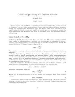
as a function of θ. Figure 1 illustrates the relationship between a hypothetical joint distribution p(θ, y) and
the conditional distribution p(θ|y = 3).
Practically, the definition of conditional probability tells us that joint distributions factor into a condi-
tional distribution times a marginal. Of course the factorization can go in either direction.
p(θ, y) = p(θ|y)p(y) = p(y|θ)p(θ).
Rearranging terms gives us Bayes’ rule
p(θ|y) =
p(y|θ)p(θ)
p(y)
. (1)
Because p(y), the marginal distribution of the data, is often hard to compute, Bayes’ rule is sometimes
written as
p(θ|y) ∝ p(y|θ)p(θ). (2)
The distribution p(θ) is called the prior distribution, or just “the prior,” p(y|θ) is the likelihood function,
and p(θ|y) is the posterior distribution. Thus Bayes’ rule is often verbalized as “the posterior is proportional
to the likelihood times the prior.”
1

2. y
−4
−2
0
2
4
6
8
theta
−4
−2
0
2
4
6
8
Density
0.00
0.02
0.04
0.06
yθ
0.005
0.01
0.015
0.02
0.025
0.03
0.035
0.04
−4 −2 0 2 4 6 8
−4−202468
(a) (b)
−4 −2 0 2 4 6 8
0.0000.0050.0100.0150.020
θ
jointdensity
−4 −2 0 2 4 6 8
0.00.10.20.30.4
θ
conditionaldensity
(c) (d)
Figure 1: Panels (a) and (b) show two different views of the joint density of θ and y. Panel (c) shows the vertical
slice of the joint density where y = 3. Panel (d) shows the conditional density p(θ|y = 3), which differs from panel
(c) only in the vertical axis labels.
2

3. Interpretation
Perhaps even more important than how to compute these probability distributions is how to interpret them.
Both the prior and posterior distribution measure one’s belief about the value of θ. The prior describes your
belief before seeing y. The posterior describes your belief after seeing y. Bayes’ theorem tells us the process
of learning about θ when y is observed.
If we think of a particular numerical value of θ as the parameters of a statistical model, then distributions
over θ are describing which sets of models are more and less likely to be correct. This is different than
frameworks that seek to identify “the model” by optimizing some criterion (such as likelihood). By working
with distributions over the space of models, Bayes handles the notion of “model uncertainty” gracefully, in
a way that classical methods struggle with. For example, both Bayesian and classical inference can describe
the uncertainty about a scalar parameter using an interval, and these intervals often agree. However, Bayes
specifies which parts of that interval are more or less likely, which confidence intervals don’t do. But that’s
just about reporting uncertainty. Bayes also allows you to average over a large group of models (represented
by the posterior distribution) in order to make better predictions than you could with a single model. The
advantages of Bayes can be hard to see in simple examples where Bayesian and classical approaches tend
to agree, but Bayes’ ability to handle model uncertainty is increasingly helpful as models become more
complicated.
The next section illustrates Bayes rule with a worked (simple) example.
3