group project

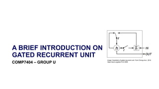
1. A BRIEF INTRODUCTION ON
GATED RECURRENT UNIT
COMP7404 – GROUP U
Image: Illustration of gated recurrent unit. From Chung et al., 2014:
https://arxiv.org/abs/1412.3555

2. AGENDA
1) A Quick Recap on Deep Learning Architectures
① Standard Neural Network (NN)
② Recurrent Neural Network (RNN)
2) A Deep Dive in Gated Recurrent Unit (GRU)
3) Rainfall Project Overview
① Competition Overview
② Source Data
③ Code and Demo: Rainfall Prediction
4) Q&A

3. LIMITATIONS OF STANDARD NEURAL
NETWORK
Source: A Critical Review of Recurrent Neural Networks for Sequence Learning, Lipton et al., 2015; Simulation of Neural Networks (in German) (1st ed.)., Zell, Andreas, 1994
Major Constraints:
 Input and output of fixed length; not
efficient with sequential data
 Do not well exploit features learned
previously
Image: Coursera: Sequence Models, Andrew Ng
Image: Wrist mounted device sleep graph, Lucid Dreaming App
Est-ce que vous
êtes prêt?
Are you ready?

4. RECURRENT NEURAL NETWORK (RNN)
Source: Understanding LSTM Networks, Olah, 2015; A Critical Review of
Recurrent Neural Networks for Sequence Learning, Lipton et al,. 2015;
The Unreasonable Effectiveness of Recurrent Neural Networks, Andrej
2015
 Has loops to deal with sequential data
 Can handle vectors of variable length
10/04/2018 Predicting E-commerce Consumer Behavior using Recurrent Neural Networks
Figure 2 showssome output h, we call thisthe hidden state of the cell.
So, what exactly are cells? Let’shave quick look at the two cell
architecturesmentioned above; LSTM and GRU. We will be testing both
architectureswhen training the models.
Long Short-Term Memory (LSTM)
The Long Short-Term Memory (LSTM) cell, like the basic cell,
computesa new state and an output from an input and the previous
state. The (hidden) state of LSTM issplit in two vectors, one for short-
term state and one for long-term state. Figure 3 illustratesthe
architecture of the LSTM cell. In gure 3, cisthe long-term state and h
isthe short-term state. LSTM receivesboth short-term and long-term
statesfrom previoustimesteps[5].
Figure 2: Cell folded/unfolded. Inspired by Aurélien Géron.
Recurrent architecture
10/04/2018 Predicting E-commerce Consumer Behavior using Recurrent Neural Networks
Figure 2 showssome output h, we call thisthe hidden state of the cell.
So, what exactly are cells?Let’shave quick look at the two cell
architecturesmentioned above; LSTM and GRU. We will be testing both
architectureswhen training the models.
Long Short-Term Memory (LSTM)
TheLong Short-Term Memory (LSTM) cell, like thebasic cell,
computesa new state and an output from an input and the previous
state. The (hidden) state of LSTM issplit in two vectors, onefor short-
term state and onefor long-term state. Figure3 illustratesthe
architectureof theLSTM cell. In gure 3, cisthe long-term state and h
isthe short-term state. LSTM receivesboth short-term and long-term
statesfrom previoustimesteps[5].
Figure 2: Cell folded/unfolded. Inspired by Aurélien Géron.#Update the hidden state
𝒉 𝒕 = 𝒇 𝑾(𝒙)
. 𝒙 𝒕 + 𝑽(𝒉)
. 𝒉 𝒕−𝟏
#Compute the output vector
𝑦𝑡 = 𝑔(𝑊(𝑦)
. ℎ 𝑡)
Notations
𝑥𝑡 = input at time t
ℎ 𝑡 = hidden state at time t
𝑦𝑡 = output at time t
f = activation functionliketanh
g = activation function for the output like a sigmoid
𝑊(𝑥)
, 𝑉(ℎ)
, 𝑊(𝑦)
= parameters
(Like standard RNN )
Image classification
Sentiment analysis,
video recognition
Text translationMusic
generation

5.  Unable to handle the “long-term dependencies”
well in practice  “Vanishing Gradient” It was a handwritten
application from Steve
Jobs for jobs in HP. We
use online application
for jobs nowadays. How
do jobs and career
mean for college
graduates? Those who
have read the
bibliography of Jobs
may have a different
viewpoint …
Loops make it a longer
path and more
complicated to
calculate the derivative
Limitations with RNNs
Solution:
Use a more sophisticated architecture which allows for shorter path and less multiplication to calculate the gradient.

6.  Learns how to keep memories for long distance dependencies
 Avoid vanishing gradient problem
mer Behavior using Recurrent Neural Networks
thisthe hidden state of the cell.
quick look at the two cell
and GRU. We will be testing both
s.
STM)
nspired by Aurélien Géron.
g E-commerce Consumer Behavior using Recurrent Neural Networks
output h, we call thisthe hidden state of the cell.
ells? Let’shave quick look at the two cell
ed above; LSTM and GRU. We will be testing both
aining the models.
Memory (LSTM)
Memory (LSTM) cell, like the basic cell,
and an output from an input and the previous
Cell folded/unfolded. Inspired by Aurélien Géron.
Equations
Different diagrams in the literature :
Update gate 𝒛𝒕 = 𝑓 𝑊(𝑧)
. 𝒙 𝒕 + 𝑉(𝑧)
. 𝒉 𝒕−𝟏
Reset gate 𝒓 𝒕 = 𝑓 𝑊(𝑟)
. 𝒙 𝒕 + 𝑉(𝑟)
. 𝒉 𝒕−𝟏
Reset gate memory 𝒉 𝒕 = 𝑔 𝑊(ℎ)
. 𝒙 𝒕 + 𝑉(ℎ)
. 𝒓 𝒕 ∗ 𝒉 𝒕−𝟏
Memory to transmit 𝒉 𝒕 = (1 − 𝒛𝒕)∗ 𝒉 𝒕−𝟏 + 𝒛𝒕 ∗ 𝒉 𝒕
Gated Recurrent Unit (GRU)
11/04/2018 Understanding GRU networks – Towards Data Science
https://towardsdatascience.com/understanding-gru-networks-2ef37df6c9be 5/14
First, let’sintroducethe notations:
If you are not familiar with theabove terminology, I recommend
watching these tutorialsabout “sigmoid” and “tanh” function and
“Hadamard product” operation.
#1. Update gate
We start with calculating theupdate gate z_t for time step t using the
formula:
Gated Recurrent Unit
12/04/2018 Predicting E-commerce Consumer Behavior using Recurrent Neural Networks
https://blog.nirida.ai/predicting-e-commerce-consumer-behavior-using-recurrent-neural-networks-36e37f1aed22 9/43
Figure 4 illustratestheGRU cell. In GRU, both state vectorsof the LSTM
havebeen merged into a singlevector, h. Instead of threegate
controllers, GRU usestwo; one controlling both the forget gate and the
input gate, while thereisno output gate. Thefull state vector isthe
output at every timestep.
Figure 4: GRU cell. Inspired by Christopher Olah.
Jobs is founder of a company, which company has its headquarter … . Jobs …
𝑧𝑡 = 1
ℎ 𝑡 = 1 … … … … ℎ 𝑡 = 1
Source: Cho et al. 2014, Coursera: Sequence Models, Andrew Ng

7. COMPETITION: HOW MUCH DID IT RAIN?
 https://www.kaggle.com/c/how-much-did-it-rain-ii/data
 Our solution
o Goal: showcase the application of GRU
o Methodology: train GRU using the radar snapshot data in
order to predict the rainfall
o Tools: Keras
 Data preprocessing challenges
o Irregular radar measurement times
o Outliers
o Overfitting
 Training data and test data may not be fully independent
Source: www. kaggle.com/c/how-much-did-it-rain-ii/data;
Scripts and sources (incl.
image, script quotation,
etc.) to be updated / Danny

8. TRAINING DATA
Training data sample:
Source: www. kaggle.com/c/how-much-did-it-rain-ii/data;
Scripts and sources (incl.
image, script quotation,
etc.) to be updated / Danny

9. DATA PREPROCESSING AND TESTING
Source: www. kaggle.com/c/how-much-did-it-rain-ii/data;
Scripts and sources (incl.
image, script quotation,
etc.) to be updated / Danny

10. CODE IMPLEMENTATION
Source: []
Slides, scripts and sources
(incl. image, script
quotation, codes, etc.) to be
updated / Paul

11. DEMO
Source: []
Items to be included in GitHub uploads:
• Demo with source and all dependencies and detailed instructions in
markdown format on how to run the demo to be uploaded as a single
zip file.
• Please ensure that the instructions on how to run the demo are
sufficiently detailed. You won’t be able to get a good grade if we are
not able to run you demo.
Items to be included in this PPT:
• The presentation must include this live demo. If a live demo is not
possible, a video demo can be presented. The file size limit for this zip
file is 100MB.
• A link to GitHub version. The link should be included as a QR code in
this PPT.
Slides, scripts and sources
(incl. image, script
quotation, codes, etc.) to be
updated / Paul

12. Q & A