1. Journal of Biogeography (J. Biogeogr.) (2007) 34, 1907–1915
ORIGINAL A comparison of altitudinal species
ARTICLE
richness patterns of bryophytes with
other plant groups in Nepal, Central
Himalaya
Oriol Grau1,2*, John-Arvid Grytnes3 and H. J. B. Birks2,3,4
1
Departament de Biologia Vegetal, Universitat ABSTRACT
de Barcelona, Av. Diagonal 645, 08028,
Aim To explore species richness patterns in liverworts and mosses along a central
Barcelona, Catalonia, Spain, 2Bjerknes Centre
for Climate Research, University of Bergen,
Himalayan altitudinal gradient in Nepal (100–5500 m a.s.l.) and to compare these
´
Allegaten 55, N-5007, Bergen, Norway, patterns with patterns observed for ferns and flowering plants. We also evaluate
3
Department of Biology, University of Bergen, the potential importance of Rapoport’s elevational rule in explaining the observed
´
Allegaten 41, N-5007, Bergen, Norway, richness patterns for liverworts and mosses.
4
Environmental Change Research Centre, Location Nepal, Central Himalaya.
University College London, London WC1E
6BT, UK Methods We used published data on the altitudinal ranges of over 840 Nepalese
mosses and liverworts to interpolate presence between maximum and minimum
recorded elevations, thereby giving estimates of species richness for 100-m
altitudinal bands. These were compared with previously published patterns for
ferns and flowering plants, derived in the same way. Rapoport’s elevational rule
was assessed by correlation analyses and the statistical significance of the observed
correlations was evaluated by Monte Carlo simulations.
Results There are strong correlations between richness of the four groups of
plants. A humped, unimodal relationship between species richness and altitude
was observed for both liverworts and mosses, with maximum richness at 2800 m
and 2500 m, respectively. These peaks contrast with the richness peak of ferns at
1900 m and of vascular plants, which have a plateau in species richness between
1500 and 2500 m. Endemic liverworts have their maximum richness at 3300 m,
whereas non-endemic liverworts show their maximum richness at 2700 m. The
proportion of endemic species is highest at about 4250 m. There is no support
from Nepalese mosses for Rapoport’s elevational rule. Despite a high correlation
between altitude and elevational range for Nepalese liverworts, results from null
simulation models suggest that no clear conclusions can be made about whether
liverworts support Rapoport’s elevational rule.
Main conclusions Different demands for climatic variables such as available
energy and water may be the main reason for the differences between the
observed patterns for the four plant groups. The mid-domain effect may explain
part of the observed pattern in moss and liverwort richness but it probably only
works as a modifier of the main underlying relationship between climate and
species richness.
*Correspondence: Oriol Grau, Departament de Keywords
`
Biologia Vegetal, Unitat de Botanica, Universitat
Altitudinal gradient, bryophytes, elevational gradient, endemism, Himalaya,
de Barcelona, Av. Diagonal, 645, 08028,
Barcelona, Catalonia, Spain. liverworts, mid-domain effect, mosses, Rapoport’s elevational rule, species
E-mail: grau.oriol@gmail.com richness.
ª 2007 The Authors www.blackwellpublishing.com/jbi 1907
Journal compilation ª 2007 Blackwell Publishing Ltd doi:10.1111/j.1365-2699.2007.01745.x

2. O. Grau, J.-A. Grytnes and H. J. B. Birks
elevational ranges of species is bounded by the highest and
INTRODUCTION
lowest elevations, so-called hard boundaries. Contrary to
The Himalaya contain the highest mountains in the world and Rapoport’s rule, the hard-boundary hypothesis predicts that
a very wide range of ecoclimate zones (Dobremez, 1976). These species ranges at higher elevations are narrow (Bhattarai &
mountains are therefore an excellent system for evaluating Vetaas, 2006). In the present study these two hypotheses are
ecological and biogeographical patterns and theories of species discussed in addition to climate as explanatory factors for the
¨
richness (Korner, 2000). Many studies have investigated observed altitudinal patterns of bryophyte richness.
patterns of plant species richness along altitudinal gradients In summary, we have the following aims: (1) to describe the
¨ ´
(e.g. Ohlemuller & Wilson, 2000; Gomez et al., 2003; Grytnes, richness pattern of liverworts and mosses along the altitudinal
2003; Oommen & Shanker, 2005; Kluge & Kessler, 2006). In gradient in Nepal; (2) to compare the altitudinal patterns of
many cases, a mid-altitude peak in species richness has been species richness of liverworts and mosses with the patterns
found (Rahbek, 2005). However, a linear decrease of richness found for vascular plants and ferns in the same area; (3) to
with altitude has also been found in some studies (e.g. Stevens, compare the altitudinal patterns in richness of endemic
1992; Rey Benayas, 1995; Brown & Lomolino, 1998; Korner, ¨ liverworts with richness patterns of non-endemic liverworts;
2002). Factors causing variation in species richness may differ and (4) to evaluate the potential importance of Rapoport’s
between different organisms, resulting in different patterns elevational rule and the mid-domain effect in explaining
(Kessler, 2000; Bhattarai & Vetaas, 2003; Grytnes et al., 2006). liverwort and moss species richness along the altitudinal
Comparing altitudinal richness patterns between different gradient in Nepal.
organisms along the same gradient may therefore provide clues
to what determines species richness patterns at broad scales
METHODS
(Lomolino, 2001). In Nepal, species richness patterns along
altitudinal gradients have been analysed for vascular plant
Location and biogeography of the study area
species and fern species. A humped relationship was found for
both vascular plants and ferns (Vetaas & Grytnes, 2002; The Himalayan altitudinal gradient is the longest bioclimatic
Bhattarai & Vetaas, 2003; Bhattarai et al., 2004). In this study gradient in the world extending from 60 m a.s.l. to more than
we focus on altitudinal patterns in liverwort and moss species 8000 m a.s.l. within 150–200 km south to north; it comprises
richness in the same area and compare the observed patterns in extensive tropical/subtropical, temperate, subalpine and alpine
species richness with the richness patterns for vascular plants climatic zones (Bhattarai et al., 2004).
and ferns. Our study area is in Nepal, which covers 900 km from east
Endemic species are of a particular interest in conservation to west in the Central Himalaya (80º04¢–88º12¢ E, 26º22¢–
and management and in biogeography because patterns in 30º27¢ N). The Himalaya consist of three ranges running
range-restricted species may reveal insights into processes of south-east to north-west in Nepal: the Siwalik range (maxi-
speciation. Vetaas & Grytnes (2002) studied the richness of mum 1000–1500 m), the Mahabharat range (maximum 2700–
endemic vascular plants in relation to altitude in Nepal. They 3000 m) and the Great Himalaya (5000–8000 m) (Hagen,
found an elevated number of endemic vascular plant species 1969; Manandhar, 1999; Bhattarai et al., 2004).
between 3800 and 4200 m, while the fraction of endemics Beug & Miehe (1999) present a cross-section of the major
increased linearly from the lowlands to the highest altitudes. In vegetation types in Central Nepal in relation to altitude,
this study we compare these observations with the altitudinal topography and climate. The principal factors governing the
patterns of Nepalese endemic liverworts. Mosses have too few vegetation zonation are altitude and the duration of cloud
endemics in Nepal for such an analysis. cover and mist. According to their scheme, forests of the
Climate, productivity and other energy-related variables are lower foothills are represented by south-eastern impoverished
commonly proposed to explain species richness patterns along stands of Asian Dipterocarpaceae forest dominated by Shorea
altitudinal gradients (Rahbek, 1997). Other hypotheses include robusta. Bryophyte growth is generally not great in these
‘Rapoport’s rule’ and the ‘mid-domain effect’. Rapoport’s tropical forests. The vegetation above 1000 m is generally
elevational rule proposes that there is a positive correlation dominated by lauraceous trees (e.g. Schima wallichii, Castan-
between elevation and the elevational range of species (Stevens, opsis indica, Castanopsis tribuloides), which form subtropical
1992). This is usually explained by the fact that species evergreen forests that vary in composition from east to west.
occurring at high elevations must be able to withstand a broad Bryophytes are present but are not luxuriant. There is a
range of climatic conditions and this leads to a wide elevational striking change in the evergreen forests below and above
range. This will, in turn, lead to more species because of a 2000 m, associated with the average altitude of the lower
spillover effect around the range edges called a rescue effect condensation level of the cloud belt. The lower cloud-forest
(Stevens, 1992). Colwell & Hurtt (1994) proposed the mid- belt (2000–2500 m) is dominated by Pinus wallichiana–Quercus
domain effect to explain mid-elevation peaks in species rich- lanata (2000–2500 m), Lithocarpus elegans (2000–2300 m) and
ness. They suggest that mid-elevation peaks in species richness Quercus glauca (2100–2500 m), and is characterized
arise because of the increasing overlap of species ranges by abundant ferns, epiphytic orchids and evergreen ferns,
towards the centre of the domain, as the extent of the and large foliose lichens (e.g. Lobaria spp.). The middle
1908 Journal of Biogeography 34, 1907–1915
ª 2007 The Authors. Journal compilation ª 2007 Blackwell Publishing Ltd

3. Altitudinal species richness patterns of bryophytes in Nepal
cloud-forest belt (2500–3000 m) is dominated by Quercus
Data analysis
semecarpifolia–Tsuga dumosa forests, and supports abundant
Calypothercium, Meteorium and Barbella beard-mosses. In the The elevational gradient was divided between 100 and 5500 m
upper cloud-forest belt (3000–4200 m) Abies spectabilis– for liverworts and between 100 and 5000 m for mosses.
Betula utilis forests are found, along with abundant tufts Between the upper and lower elevational limits, species were
and mats of epiphytic liverworts (e.g. Herbertus spp., Plagio- counted at every 100-m interval in the same way as in Vetaas &
chila spp.). Bryophytes, both mosses and liverworts, dominate Grytnes (2002) and Bhattarai et al. (2004). This gives an
the ground layer and form extensive carpets over boulders and estimate of gamma diversity, defined as the total richness of an
tree bases. Epiphytic beard-lichens (Usnea spp.) can be locally entire elevational zone (sensu Lomolino, 2001). In this study,
abundant, especially in openings in the upper cloud-forest. species richness (Peet, 1974) is defined as the number of
Large leafy liverworts (e.g. Schill & Long, 2003; Long, 2005) species present in each 100-m band. When estimating species
can also occur frequently in the subalpine Rhododendron– richness it was assumed that species were present in all
Potentilla–Kobresia–Juniperus communities, especially on steep elevational zones between the range limits (interpolation). This
north- or east-facing slopes up to an altitude of about may create an artificially humped pattern (Grytnes & Vetaas,
4800 m. Above that, up to 5200 m, the vegetation gradually 2002), but in this study the main aim is to compare elevational
becomes open and the cover and number of species of mosses species richness patterns for different plant groups that are all
and lichens often exceed the cover and richness of flowering treated in the same way so as to highlight similarities or
plants (Beug & Miehe, 1999). differences in where maximum species richnesses are found.
Any differences in the optimal altitudes for species richness for
the different groups are probably not an artefact of the
Data sources
interpolation method used. In addition, bryophytes are rarely
For quantifying the richness patterns of mosses and liverworts found at the lowermost elevations, and because interpolations
in Nepal we used the data on elevational ranges published in will have their largest effect on the observed pattern at the
Mosses of Nepal (Kattel & Adhikari, 1992) and Liverworts of lowermost and uppermost elevations, the use of interpolation
Nepal (Kattel, 2002). The maximum and minimum altitudes will probably not have a significant impact on the resulting
known for each species are given and endemic species are also bryophyte richness patterns.
noted. Elevational limits are given for 368 liverwort and To describe the species richness patterns in relation to
480 moss taxa, from which in a few cases varieties or altitude, a generalized additive model (GAM) with a cubic
subspecies are considered as separate taxa. In this study we smooth spline (Hastie & Tibshirani, 1990), as implemented in
use the term ‘species richness’ for the number of taxa. The R 2.2.1 (R Development Core Team, 2004) was used. The
exact number of endemic mosses and liverworts growing in GAM approach is especially useful for data exploration as it
Nepal is not known. Chaudhary (1998) reported about makes no a priori assumptions about the type of relationship
30 endemic bryophyte species in Nepal, of which only four being modelled. The GAM approach contrasts with the
were mosses. Kattel (2002) lists a slightly higher number of generalized linear model approach where a priori assumptions
endemic bryophytes, with 33 endemic liverwort species and about the relationships being modelled (e.g. a symmetrical
three mosses. Knowledge about bryophytes in Nepal is humped relationship) are required. Richness patterns for
continually increasing. Species new to Nepal are being mosses, liverworts, vascular plants and ferns were regressed
regularly reported (e.g. Zhu & Long, 2003; Long, 2005, against altitude and plotted for comparison.
2006; Wilbraham & Long, 2005) and previously undescribed Initially, species richness data were considered to follow a
species are also being found in Nepal (e.g. Ochra, 1989; Poisson distribution as is usual for variables with discrete
Furuki & Long, 1994; Long, 1999; Grolle et al., 2003). values (McCullagh & Nelder, 1989). However, a quasi-Poisson
Taxonomic revisions (Schill & Long, 2003; Long et al., 2006) distribution was used because of overdispersion. The propor-
and the resolution of synonyms and erroneous records (e.g. tion of endemic vs. non-endemic liverworts was assumed to
Long, 1995) are also improving knowledge about the follow a binomial distribution with the number of endemics as
composition of Nepal’s moss and liverwort floras. At present successes and the number of non-endemics as failures. For the
there are no published checklists and altitudinal distributional quasi-Poisson analyses a logarithmic link was used, and for the
data that update Kattel & Adhikari (1992) and Kattel (2002). binomial analyses a logit link was used.
Given the current state of knowledge about Nepalese Rapoport’s elevational rule was evaluated by correlating
bryophytes, these two monographs (Kattel & Adhikari, mean species altitudinal ranges for all species found in each
1992; Kattel, 2002) are considered adequate for this broad- 100-m elevational interval with altitude. This has been
scale study of species richness patterns in relation to altitude criticized on several grounds (Colwell & Lees, 2000). In an
and for comparison with richness patterns in other plant attempt to allow for possible artefacts we compared our
groups (D.G. Long, personal communication). Data for fern observed correlations with the results from Monte Carlo
and vascular plant species richness were obtained from simulations under a null model. The null model was made by
Bhattarai et al. (2004) and Vetaas & Grytnes (2002), randomly choosing one of the feasible observed altitudinal
respectively. ranges for each of the observed mid-points taking into account
Journal of Biogeography 34, 1907–1915 1909
ª 2007 The Authors. Journal compilation ª 2007 Blackwell Publishing Ltd

4. O. Grau, J.-A. Grytnes and H. J. B. Birks
the boundary constraints. This approach is the same as Model
3 in Colwell & Hurtt (1994). The simulation was run 9999
times and for each permutation the same correlation between
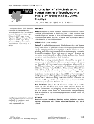
200
mean altitudinal range and altitude was calculated. A one-
sided test was performed based on these simulations because
Rapoport’s rule predicts a positive correlation between mean
Species richness of mosses
150
altitudinal range and altitude. An empirical P-value was
derived from the number of simulations with a positive
correlation larger than (or equal to) the observed value.
100
Due to difficulties in separating the effect of interpolation
and undersampling from the mid-domain effect (Grytnes &
Vetaas, 2002; Zapata et al., 2003), no specific randomizations
50
were performed to test for this in this study. The mid-domain
effect is therefore only discussed briefly in the discussion and
compared with the simulations made in Grytnes & Vetaas
0
(2002) for vascular plants along the same gradient. Although
this is not optimal, we refrain from ‘guessing’ how complete 0 1000 2000 3000 4000 5000 6000
the biological sampling has been in this case. As a result, the Altitude (m)
assumptions and simulations made in Grytnes & Vetaas (2002) Figure 2 Moss richness in relation to altitude (m) in Nepal. The
may therefore be as reliable as anything else, given the current fitted line represents a GAM model with a cubic smooth spline.
state of knowledge of bryophyte recording in Nepal.
1200
RESULTS 200
Both moss and liverwort species richness have a clear humped
1000
relationship with altitude, with a very marked maximum at
middle altitudes (Figs 1 & 2). Mosses have highest richness
150
800
values at around 2500 m, whereas non-endemic liverworts
Species richness
reach their maximum at a slightly higher altitude, at around
2700 m. Endemic liverworts show their maximum richness at
600
100
even higher altitudes, at about 3300 m.
When comparing species richness of liverwort, moss, fern
400
and vascular plant with each other (Fig. 3), all show a
50
200
20
0
150
0 1000 2000 3000 4000
Altitude (m)
15
Figure 3 Fern (º), moss (h) and liverwort (D) richness (values
on the left-hand axis) and vascular plant richness ( , values on the
100
Species richness
right-hand axis) in relation to altitude (m) in Nepal. The fitted
lines represent a GAM model with a cubic smooth spline.
10
markedly humped relationship with altitude. This may be a
50
result of underlying ecological patterns or it may, at least
5
partly, be a result of using interpolation with data that are
undersampled. We therefore focus most on the relative
location of the peak in species richness when comparing the
0
0
altitudinal patterns of the different plant groups. Maximum
0 1000 2000 3000 4000 5000 6000 species richness for vascular plants is between 1500 and
Altitude (m)
2500 m. Fern species richness peaks at 1900 m, mosses at
Figure 1 Non-endemic liverwort richness (·, values on the left- 2500 m and liverworts at 2800 m (if endemic and non-
hand axis) and endemic liverwort richness (º, values on the right- endemic taxa are not distinguished). There is a strong
hand axis) in relation to altitude (m) in Nepal. The fitted lines correlation between richness for the different groups (Table 1),
represent a GAM model with a cubic smooth spline. being highest between mosses and liverworts and lowest
1910 Journal of Biogeography 34, 1907–1915
ª 2007 The Authors. Journal compilation ª 2007 Blackwell Publishing Ltd

5. Altitudinal species richness patterns of bryophytes in Nepal
Table 1 Correlation between species richness along the altitudinal
gradient of Nepal for different groups of plants. All correlations
2500
(Pearson’s product moment correlation) are statistically signifi-
cant (P < 0.05).
Mean altitudinal range
Mosses Liverworts Ferns
2000
Liverworts 0.89 – –
Ferns 0.68 0.34 –
Vascular plants 0.74 0.59 0.74
1500
between ferns and liverworts. The maximum elevation for
mosses is achieved by Grimmia somervillii at 5100 m (Kattel &
Adhikari, 1992). The highest elevation for liverworts is
achieved by Anastrophyllum assimile, which reaches 5450 m
(Kattel, 2002).
The proportion of endemic to non-endemic liverworts is
0 1000 2000 3000 4000 5000
highest around 4250 m, with a steady increase starting at Altitude (m)
around 1200 m, where the first endemic species is found
(Fig. 4). The decrease in the proportion of endemics at the Figure 5 Liverwort altitudinal range (m) versus altitude (m) in
Nepal. The fitted line represents an ordinary least square (OLS)
highest altitudes is a consequence of the lack of endemic
linear regression.
liverworts over 5000 m.
According to our data, the altitudinal ranges of liverworts
a marginal P-value makes it impossible to accept or reject
show a statistically significant increase with altitude as assessed
unambiguously the relevance of Rapoport’s rule on Nepalese
by classical statistical tests (Fig. 5) (r = 0.63, P < 0.01)
liverworts. Since this P-value was very close to the chosen
supporting Rapoport’s elevational rule. In the lower altitudinal
significance level at 0.05, we performed a jack-knife (leave-one-
bands, the average altitudinal range is around 1500 m, whereas
out) analysis to investigate if the P-value was due to a single
the species found in the highest altitudinal bands have an
species. This was done by repeating the permutation analysis
average altitudinal range greater than 2000 m. At first glance
leaving out one species at the time (to reduce computing time
such results appear to support Rapoport’s elevational rule.
we did 999 permutations for each species). For two of the
However, after running the Monte Carlo simulations, it is
species the P-value became lower than what is observed for all
found that such a significant positive correlation between
species [one of these was barely below 0.05 (0.042)]. For all the
elevational ranges and altitude could have been obtained by
remaining species the P-values from the jack-knife analyses
chance, because the empirically derived P-value is 0.063. Such
were higher than the P-value for all species. Mosses showed no
significant positive correlation between mean altitude ranges
and altitude (plot not shown, r = )0.07, P > 0.1), and the
permutations confirmed this with an empirical P-value of
0.20
0.616. Thus, moss richness does not support Rapoport’s
elevational rule either.
0.15
Proportion of endemics
DISCUSSION
Mid-elevation peak in species richness
0.10
Bryophyte richness varies strongly with altitude in Nepal
(Figs 1 & 2), similarly to the pattern observed for vascular
0.05
plants (Grytnes & Vetaas, 2002; Oommen & Shanker, 2005;
Bhattarai & Vetaas, 2006) and ferns (Bhattarai et al., 2004). In
all cases, the patterns show a mid-elevation peak in species
richness. A hump-shaped relationship of bryophyte richness
0.00
with altitude has also been found in other areas, such as in the
0 1000 2000 3000 4000 5000 tropics (Gradstein & Pocs, 1989; Wolf, 1993). Andrew et al.
Altitude (m)
(2003) also reported a unimodal response in some mountains
Figure 4 Proportion of endemic versus non-endemic liverwort in Tasmania, although it was not general for all sites studied.
species in relation to altitude (m) in Nepal. The fitted line rep- When comparing our results to the cross-section of the
resents a GAM model with a cubic smooth spline. vegetation in the altitudinal belts of Central Nepal described by
Journal of Biogeography 34, 1907–1915 1911
ª 2007 The Authors. Journal compilation ª 2007 Blackwell Publishing Ltd

6. O. Grau, J.-A. Grytnes and H. J. B. Birks
Beug & Miehe (1999), ferns have their maximum richness temperature and PET values, resulting in higher water stress.
100 m below the altitude where the lower cloud-forest belt The decrease in species richness at high altitudes is probably
starts; moss richness peaks exactly at the altitude where the due to ecophysiological constraints, such as reduced growing
middle cloud-forest belt starts and liverwort richness peaks season, low temperatures, frost susceptibility and low energy
about 200 m below the lower limit of the upper cloud-forest ¨
(Brown, 2001; Korner, 2003).
belt. According to data from Bhattarai et al. (2004), vascular One additionally possible important factor for the low
plants in Nepal have a maximum richness at around 14–17°C species richness at high altitudes is that a high proportion of
mean annual temperature and 250–330 growing days, whereas the Nepalese bryophytes have been described as epiphytes or
ferns have a maximum richness at around 15°C mean annual are associated with logs and fallen trees (Kattel, 2002; H.J.B.
temperature and 300 growing days. Based on climatic data Birks, personal observation). Forests in the Nepalese foothills
from Bhattarai et al. (2004), we estimate that maximum (2500–4000 m) provide a range of habitats for mosses and
species richness for mosses occurs at around 13°C and 265 liverworts including rocks, logs, trunks, branches, twigs and
growing days, whereas maximum liverwort richness occurs at leaves, all of which support bryophytes, especially in the zone
around 10°C and 225 growing days. of strongest summer rain (up to 4000 mm) between 2500 and
Maximum liverwort richness is found at lower mean annual 3600 m (Beug & Miehe, 1999). The timberline in the Nepalese
temperatures. This coincides with a short growing-season Himalaya is around 4000–4300 m (Bhattarai & Vetaas, 2006).
length and high moisture. Liverworts are particularly prevalent At this altitude there is a low bryophyte richness, which
in moist and cool habitats (Turner et al., 2006), and our suggests that the lack of forests and trees and hence the absence
findings support this. The fact that liverworts may require of important habitats may be an important reason for the
more moisture and can withstand a shorter growing season decreasing bryophyte species richness, as occurs with ferns
and low temperatures could be a possible explanation for the (Beug & Miehe, 1999; Bhattarai et al., 2004). A marked
altitudinal differences in the species richness peaks of mosses decrease in bryophyte richness towards the lowlands has also
and liverworts. been found in other vegetation types in Nepal (Bhattarai &
In order to understand how climate may explain bryophyte Vetaas, 2003, 2006; Bhattarai et al., 2004). The very small
richness patterns, it is interesting to relate climate to the number of species found in the lowlands may be due to
evolutionary adaptations of bryophytes. According to Oliver inadequate sampling or, more likely, to habitat loss. Defores-
et al. (2000), the evolution of terrestrial plants might be a tation in the lower part of Nepal started after the control of
result of changes in desiccation tolerance; as species evolved, malaria (Bhattarai et al., 2004), which contributed to extensive
vegetative desiccation tolerance was lost as increased growth habitat loss. However, several plant-hunting expeditions were
rates, structural and morphological complexity and mecha- undertaken prior to extensive deforestation (Bhattarai et al.,
nisms that conserve water within the plant and maintain 2004). In general, the richness and abundance of bryophytes
efficient carbon fixation were selected for. Oliver et al. (2000), decrease dramatically in the lowlands of Himalaya. We
after compiling several recent studies, proposed that liverworts hypothesize that the low bryophyte richness observed here is
were the most primitive group of land plants, and closely not only caused by habitat loss and inadequate sampling, but
related to mosses, whereas mosses were the evolutionary step may also have other explanations, for example unfavourable
prior to tracheophytes, such as ferns and vascular plants. macro- or microclimate, including high PET conditions
Assuming that the driving force of terrestrial plant evolution resulting in lower water availability.
involved coping better with water stress, vascular plants should If the mid-domain effect was the sole important variable it
be better adapted to water conservation than ferns, which in would predict that all species groups should show the same
turn should be better adapted than mosses, which in turn pattern. This is not seen in this study, indicating that the mid-
should be better adapted than liverworts. Such different domain effect alone cannot explain the observed patterns.
adaptations to water stress may provide some explanations Grytnes & Vetaas (2002) argued that hard boundaries, an
for maximum species richness occurring at decreasing alti- underlying monotonic trend in species richness, incomplete
tudes, starting with liverworts at highest elevations, followed sampling and the interpolation method may, in combination,
by mosses and finally ferns and vascular plants towards lower underestimate species number at the gradient extremes, which
altitudes. The order of appearance from higher to lower may help to explain the observed pattern in species richness
altitude may reflect the order in which plant species evolved in along the altitudinal gradient in the Nepalese Himalaya
the past according to the phylogeny presented by Oliver et al. (Grytnes & Vetaas, 2002). However, the clear peaks in species
(2000). The presumably less-evolved adaptation to water stress richness observed for bryophytes do not correspond to any of
in liverworts is associated with higher species richness in areas the simulations made in Grytnes & Vetaas (2002), again
where potential evapotranspiration (PET), the number of indicating that the mid-domain effect may not be important in
growing days and the mean annual temperature are low, creating the observed patterns for bryophytes. At broad scales,
resulting in high moisture. On the other hand, the progres- the influence of the mid-domain effect may be limited and
sively better adaptations of mosses, ferns and vascular plants to overshadowed by area, temperature or energy-related factors,
water stress allow them to have peak richness at altitudes with whereas at intermediate scales the mid-domain effect might
gradually higher number of growing days, mean annual offer a better explanation (Oommen & Shanker, 2005).
1912 Journal of Biogeography 34, 1907–1915
ª 2007 The Authors. Journal compilation ª 2007 Blackwell Publishing Ltd

7. Altitudinal species richness patterns of bryophytes in Nepal
Differences in scale might be the reason why in some studies
Rapoport’s elevational rule
the mid-domain effect provides more powerful explanations
for observed richness patterns than climatic factors or vice In some studies, Rapoport’s rule has been reported to apply to
versa. trees, seaweeds, arthropods, marine and terrestrial molluscs,
fish, amphibians, reptiles, birds and mammals (Pianka, 1989;
Stevens, 1989; Gaston, 2003; Almeida-Neto et al., 2006;
Endemism
Hausdorf, 2006; Morin & Chuine, 2006). However, Bhattarai
There is no overlap between the peak of maximum endemic & Vetaas (2006) studied tree species richness in Nepal and
liverwort species at 3300 m and the maximum of non-endemic found no support for Rapoport’s elevational rule since
liverwort species at 2700 m, with a striking 600 m difference altitudinal ranges were narrow at both ends of the gradient
between the peaks (Fig. 1). Similar results have been found for and wide at middle elevations. Although altitudinal ranges
endemic and non-endemic vascular plant species in Nepal increase towards higher altitudes according to our data
(Vetaas & Grytnes, 2002) and for ferns in Costa Rica (Kluge & (Fig. 5), this study gives no clear support for Rapoport’s rule
Kessler, 2006). as proposed by Stevens (1992). The Monte Carlo simulations,
A high degree of isolation generally creates endemism. which compared the observed correlations for this rule with a
Isolation is obviously more pronounced at higher altitudes, as null model, showed that such a pattern, which coincides with
the high peaks may function as islands in a ‘sea’ of lowlands. the predictions from Rapoport’s rule, could have been
In the Nepalese lowlands the environment is more similar to obtained randomly. The null model proposed no significant
the regions surrounding it and species may freely expand their difference in elevational ranges of mosses and liverworts with
ranges. The vegetation in the lowlands has been strongly altitude, and since we found a 6.3% probability that the null
influenced by human activity, and endemics may have been model corresponds to our empirical data we cannot say that
differentially extirpated compared with widespread species. Rapoport’s rule is supported for the Nepalese liverworts. In
Glaciation may add to the isolation effects at higher altitudes addition, the shift between non-endemic and endemic liver-
and may have acted as a dispersal barrier, and enhanced the wort species (Fig. 1) also does not support Rapoport’s
physical barriers created by the mountains, thereby providing elevational rule (Stevens, 1992), which proposes that endemic
a mechanism for increased isolation (Vetaas & Grytnes, 2002). species should increase towards the lowlands because, by
In addition, for vascular plants it is known that broad-scale definition, they have a narrow geographical range.
climatic dynamics can facilitate hybridization between pre- In any case, species ranges result from complex interactions
viously isolated populations, followed by polyploidy, which among many factors ranging from physiological traits to the
may result in new species adapted to conditions following complex history of speciation and dispersal, and constraints
climatic change (Stebbins, 1984). It has been proposed that resulting from continent shape (Webb & Gaston, 2003). No
polyploids have a greater resistance to the severe conditions general trends appear to exist for Rapoport’s rule for all
found at high elevations, which may have promoted biological organisms, suggesting that the factors determining
endemism at higher altitudes (Vetaas & Grytnes, 2002). There range size are complex and remain poorly understood.
is a high polyploidy ratio among neoendemic vascular plant
species both in the Himalaya and elsewhere (Kadota, 1987;
ACKNOWLEDGEMENTS
Sakya & Joshi, 1990; Nayar, 1996; Solitis et al., 1996).
Natcheva & Cronberg (2004) report the existence of We are indebted to Dr David Long (Royal Botanic Garden
polyploidy in hepatics, and suggested that several isolating Edinburgh) for helpful discussions about Nepalese bryophytes.
mechanisms that are recognized in flowering plants may Oriol Grau thanks the European Union and the Bjerknes
possibly also occur in bryophytes. Bischler & Boisselier- Centre for Climate Research (Bergen) for a Marie Curie
Dubayle (1993) showed that polyploidy also occurs in Fellowship, which made this study possible. John Birks
liverworts with restricted ranges. For these reasons, the same acknowledges Jesus College, Oxford for a Visiting Senior
processes that favour polyploidy in vascular plants may also Research Fellowship during the final work on this manuscript.
influence the number of endemic bryophytes at higher This is publication A161 from the Bjerknes Centre for Climate
altitudes in the Himalaya. Research, Bergen.
On the other hand, it is interesting to note that the highest
proportion of endemics (Fig. 4) is found at approximately
REFERENCES
4250 m, very close to the timberline in the Nepalese Himalaya,
which is at around 4000–4300 m (Bhattarai & Vetaas, 2006). Almeida-Neto, M., Machado, G., Pinto-da-Rocha, R. &
However, the flattening and estimated decrease in the Giaretta, A.A. (2006) Harvestman (Arachnida: Opiliones)
endemism ratio towards the highest altitudes should be species distribution along three Neotropical elevational
interpreted with caution because only a few species are gradients: an alternative rescue effect to explain Rapoport’s
observed at these altitudes, resulting in uncertain estimates rule? Journal of Biogeography, 33, 361–375.
of the ratio at these altitudes compared with more species-rich Andrew, N.R., Rodgerson, L. & Dunlop, M. (2003) Variation
areas. in invertebrate-bryophyte community structure at different
Journal of Biogeography 34, 1907–1915 1913
ª 2007 The Authors. Journal compilation ª 2007 Blackwell Publishing Ltd

8. O. Grau, J.-A. Grytnes and H. J. B. Birks
spatial scales along altitudinal gradients. Journal of Biogeo- Grytnes, J.A. & Vetaas, O.R. (2002) Species richness and altitude,
graphy, 30, 731–746. a comparison between simulation models and interpolated
Beug, H.J. & Miehe, G. (1999) Vegetation history and human plant species richness along the Himalayan altitudinal gra-
impact in the Eastern Central Himalaya (Langtang and dient, Nepal. The American Naturalist, 159, 294–304.
Helambu, Nepal). Dissertationes Botanicae 318. J. Cramer, Grytnes, J.A., Heegaard, E. & Ihlen, P.G. (2006) Species rich-
Berlin and Stuttgart. ness of vascular plants, bryophytes, and lichens along an
Bhattarai, K.R. & Vetaas, O.R. (2003) Variation in plant spe- altitudinal gradient in western Norway. Acta Oecologica–
cies richness of different lifeforms along a subtropical ele- International Journal of Ecology, 29, 241–246.
vation gradient in the Himalayas, east Nepal. Global Ecology Hagen, T. (1969) Report on the geological survey of Nepal.
and Biogeography, 12, 327–340. Denckschrift der Schweizerischen Naturforschenden Gesellsc-
Bhattarai, K.R. & Vetaas, O.R. (2006) Can Rapoport’s rule haft, LXXXVI/I, 185.
explain tree species richness along the Himalayan elevation Hastie, T.J. & Tibshirani, R.J. (1990) Generalized additive
gradient, Nepal? Diversity and Distributions, 12, 373–378. models. Chapman & Hall, London.
Bhattarai, K.R., Vetaas, O.R. & Grytnes, J.A. (2004) Fern Hausdorf, B. (2006) Latitudinal and altitudinal diversity pat-
species richness along a Central Himalayan elevational gra- terns and Rapoport effects in north-west European land
dient, Nepal. Journal of Biogeography, 31, 389–400. snails and their causes. Biological Journal of the Linnean
Bischler, H. & Boisselier-Dubayle, M.C. (1993) Variation in a Society, 87, 309–323.
polyploid, dioicous liverwort, Marchantia globosa. American Kadota, J. (1987) A revision of Aconitum subgenus Aconitum
Journal of Botany, 80, 953–958. (Ranunculaceae) of Eastern Asia. Sanwa Shoyaku Co.,
Brown, J.H. (2001) Mammals on mountainsides: elevational Utsunomiya, Japan.
patterns of diversity. Global Ecology and Biogeography, 10, Kattel, L.P. (2002) Liverworts of Nepal. Dambari Kattel Pub-
101–109. lishing, Kathmandu.
Brown, J.H. & Lomolino, M.V. (1998) Biogeography, 2nd edn. Kattel, L.P. & Adhikari, M.K. (1992) Mosses of Nepal. Natural
Sinauer, Sunderland, MA. History Society of Nepal, Kathmandu.
Chaudhary, R.P. (1998) Biodiversity in Nepal. Status and Kessler, M. (2000) Elevational gradients in species richness and
conservation. Know Nepal series, 17. Tecpress Books, endemism of selected plant groups in the Central Bolivian
Bangkok. Andes. Plant Ecology, 149, 181–193.
Colwell, R.K. & Hurtt, G.C. (1994) Nonbiological gradients in Kluge, J. & Kessler, M. (2006) Fern endemism and its corre-
species richness and a spurious Rapoport effect. The lates: contribution from an elevational transect in Costa
American Naturalist, 144, 570–595. Rica. Diversity and Distributions, 12, 535–545.
Colwell, R.K. & Lees, D.C. (2000) The mid-domain effect: ¨
Korner, C. (2000) Why are there global gradients in species
geometric constraints on the geography of species richness. richness? Mountains might hold the answer. Trends in
Trends in Ecology & Evolution, 15, 70–76. Ecology & Evolution, 15, 513–514.
Dobremez, J.F. (1976) Le Nepal, ´cologie et biogeographie.
´ e ´ ¨
Korner, C. (2002) Mountain biodiversity, its causes and
Centre National de la Recherche Scientifique, Paris. function: an overview. Mountain biodiversity: a global
Furuki, T. & Long, D.G. (1994) Aneura crateriformis, a new ¨
assessment (ed. by Ch. Korner and E.M. Spehn), pp. 3–20.
liverwort species from the East Himalaya and China. Journal Parthenon, Boca Raton, FL.
of Bryology, 18, 281–286. ¨
Korner, C. (2003) Alpine plant life, 2nd edn. Springer-Verlag,
Gaston, K.J. (2003) The structure and dynamics of geographic Berlin.
ranges. Oxford University Press, New York. Lomolino, M.V. (2001) Elevation gradients of species-richness,
´ ´
Gomez, D., Sese, J.A. & Villar, L. (2003) The vegetation of the historical and prospective views. Global Ecology and Bio-
alpine zone in the Pyrenees. Alpine biodiversity in Europe, geography, 10, 3–13.
Ecological Studies, Vol. 167 (ed. by L. Nagy, G. Grabherr, C. Long, D.G. (1995) The Musci Indica: its authors, types and
¨
Korner and D.B.A. Thompson) pp. 85–92. Springer-Verlag, localities. Botanical Journal of the Linnean Society, 119, 1–33.
Berlin. Long, D.G. (1999) Studies on the genus Asterella, IV. Asterella
Gradstein, S.R. & Pocs, T. (1989) Bryophytes. Tropical rain- grollei sp. nov., a new species from Eastern Asia related to
forest ecosystems: biogeographical and ecological studies, eco- the American A. palmeri. Bryologist, 102, 169–178.
systems of the World, 14 (ed. by H. Lieth and M.J.A. Long, D.G. (2005) Notes on Himalayan Hepaticae, 2: new
Werger), pp. 311–325. B. Elsevier, Amsterdam. records and extensions of range for some Himalayan leafy
Grolle, R., Schill, D.B. & Long, D.G. (2003) Notes on Gott- liverworts. Cryptogamie, Bryologie, 26, 97–107.
schelia (Jungermanniales, Lophoziaceae), with a description Long, D.G. (2006) Notes on Himalayan Hepaticae, 3: new
of G. patoniae, a new species from the East Himalaya. records and extension of range for some Himalayan and
Journal of Bryology, 25, 3–6. Chinese Marchantiales. Cryptogamie, Bryologie, 27, 119–129.
Grytnes, J.A. (2003) Species richness patterns of vascular plants Long, D.G., Paton, J.A., Squirrell, J., Woodhead, M. & Hol-
along seven altitudinal transects in Norway. Ecography, 26, lingsworth, P.M. (2006) Morphological, ecological and
291–300. genetic evidence for distinguishing Anastrophyllum joergensenii
1914 Journal of Biogeography 34, 1907–1915
ª 2007 The Authors. Journal compilation ª 2007 Blackwell Publishing Ltd

9. Altitudinal species richness patterns of bryophytes in Nepal
Schiffn. and. A. alpinum Steph. (Jungermanniopsida: Lop- Stebbins, G.L. (1984) Polyploidy and distribution of the arctic-
hoziaceae). Journal of Bryology, 28, 108–117. alpine flora: new evidence and new approaches. Botanica
Manandhar, M.S. (1999) Evolution of the Himalaya. Nepal Helvetica, 94, 1–13.
nature’s paradise (ed. by T.C. Majupuria and R.K. Maj- Stevens, G.C. (1989) The latitudinal gradient in geographical
upuria), pp. 13–17. Hillside Press Ltd, Kathmandu. range: how so many species coexist in the tropics. The
McCullagh, P. & Nelder, J.A. (1989) Generalized linear models, American Naturalist, 133, 240–256.
2nd edn. Chapman & Hall, London. Stevens, G.C. (1992) The elevational gradient in altitudinal
Morin, X. & Chuine, I. (2006) Niche breadth, competitive range: an extension of Rapoport’s latitudinal rule to altitude.
strength and range size of tree species: a trade-off based The American Naturalist, 140, 893–911.
framework to understand species distribution. Ecology Let- Turner, P.A.M., Kirkpatrick, J.B. & Pharo, E.J. (2006) Bryo-
ters, 9, 185–195. phyte relationship with environmental and structural vari-
Natcheva, R. & Cronberg, N. (2004) What do we know about ables in Tasmanian old-growth mixed eucalypt forest.
hybridisation among bryophytes in nature? Canadian Jour- Australian Journal of Botany, 54, 239–247.
nal of Botany, 82, 1687–1704. Vetaas, O.R. & Grytnes, J.A. (2002) Distribution of vascular
Nayar, M.P. (1996) Hotspots of endemic plants of India, Nepal, plants species richness and endemic richness along the Hi-
and Bhutan. Tropical Botanic Garden and Research Insti- malayan elevation gradient in Nepal. Global Ecology and
tute, Palode, Thiruvananthapuram. Biogeography, 11, 291–301.
Ochra, R. (1989) Miehea himalayana, a new species and genus Webb, T.J. & Gaston, K.J. (2003) On the heritability of geo-
of Hylocomiaceae (Musci) from the Himalayas. Nova graphic range sizes. The American Naturalist, 164, 553–566.
Hedwigia, 49, 323–332. Wilbraham, J. & Long, D.G. (2005) Zygodon Hook & Taylor
¨
Ohlemuller, R. & Wilson, J.B. (2000) Vascular plant species and Bryomaltala Goffinet (Bryopsida: Orthotrichaceae) in
richness along latitudinal and altitudinal gradients: a con- the Sino-Himalaya. Journal of Bryology, 27, 329–342.
tribution from New Zealand temperate rainforests. Ecology Wolf, J.H.D. (1993) Diversity patterns and biomass of
Letters, 3, 262–266. epiphytic bryophytes and lichens along an altitudinal gra-
Oliver, M., Tuba, Z. & Mishler, B.D. (2000) The evolution of dient in the northern Andes. Annual Report–Missouri
vegetative desiccation tolerance in land plants. Plant Ecology, Botanical Garden, 80, 928–960.
151, 85–100. Zapata, F.A., Gaston, K.J. & Chown, S.L. (2003) Mid-domain
Oommen, M.A. & Shanker, K. (2005) Elevational species models of species richness gradients: assumptions, methods
richness patterns emerge from multiple local mechanisms in and evidence. Journal of Animal Ecology, 72, 677–690.
Himalayan woody plants. Ecology, 86, 3039–3047. Zhu, R.–L. & Long, D.G. (2003) Lejeuneaceae (Hepaticae)
Peet, R. (1974) The measurement of species diversity. Annual from several recent collections from the Himalaya. Journal of
Review of Ecology and Systematics, 5, 285–307. the Hattori Botanical Laboratory, 93, 101–115.
Pianka, E.R. (1989) Latitudinal gradients in species–diversity.
Trends in Ecology & Evolution, 4, 223–223.
R Development Core Team (2004) R: a language and envi-
ronment for statistical computing. R Foundation for Statis-
tical Computing, Vienna. BIOSKETCHES
Rahbek, C. (1997) The relationship among area, elevation and
regional species richness in neotropical birds. The American Oriol Grau is a doctoral student at the Department of Plant
Naturalist, 149, 875–902. Biology, University of Barcelona. His research interests are
Rahbek, C. (2005) The role of spatial scale and the perception of vegetation dynamics, plant ecology and biogeography in alpine
large-scale species-richness patterns. Ecology Letters, 8, 224–239. and subarctic regions.
Rey Benayas, J.M.R. (1995) Patterns of diversity in the strata of
boreal montane forest in British Columbia. Journal of John-Arvid Grytnes is a post-doctoral researcher at the
Vegetation Science, 6, 95–98. University of Bergen. His research interests are all aspects of
Sakya, S.R. & Joshi, K.K. (1990) Karyomorphological studies in species richness patterns at different spatial scales. Current
some Primula species of Nepal Himalaya. Cytologia, 55, projects focus mostly on elevational richness patterns and
571–579. problems in quantifying and interpreting these patterns.
Schill, D. & Long, D.G. (2003) A revision of Anastrophyllum John Birks is a botanist at the University of Bergen and
(Spruce) Steph. (Jungermanniales, Lophoziaceae) in the University College London with research interests in Quater-
Himalayan Region and Western China. Journal of the Hat- nary palaeoecology, quantitative methods, community ecol-
tori Botanical Laboratory, 94, 115–157. ogy, vegetation dynamics, biogeography and alpine botany
Solitis, D.E., Kuzoff, R.K., Conti, E., Gornall, R. & Ferguson, (http://www.eecrg.uib.no/personal_pages/).
I.K. (1996) MatK and rbcL gene sequence data indicate that
Saxifraga (Saxifragaceae) is polyphyletic. American Journal
of Botany, 83, 371–382. Editor: Nicholas J. Gotelli
Journal of Biogeography 34, 1907–1915 1915
ª 2007 The Authors. Journal compilation ª 2007 Blackwell Publishing Ltd