

Empfohlen
Weitere ähnliche Inhalte
Was ist angesagt?
Was ist angesagt? (20)
Andere mochten auch
Ähnlich wie Income distribution
Ähnlich wie Income distribution (20)
Mehr von Gargee Ghosh
Mehr von Gargee Ghosh (7)
Kürzlich hochgeladen
Kürzlich hochgeladen (20)
Income distribution
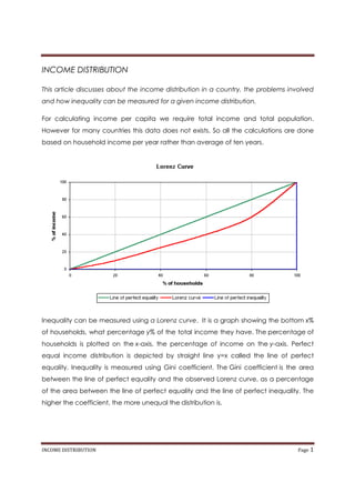
- 1. INCOME DISTRIBUTION This article discusses about the income distribution in a country, the problems involved and how inequality can be measured for a given income distribution. For calculating income per capita we require total income and total population. However for many countries this data does not exists. So all the calculations are done based on household income per year rather than average of ten years. Inequality can be measured using a Lorenz curve. It is a graph showing the bottom x% of households, what percentage y% of the total income they have. The percentage of households is plotted on the x-axis, the percentage of income on the y-axis. Perfect equal income distribution is depicted by straight line y=x called the line of perfect equality. Inequality is measured using Gini coefficient. The Gini coefficient is the area between the line of perfect equality and the observed Lorenz curve, as a percentage of the area between the line of perfect equality and the line of perfect inequality. The higher the coefficient, the more unequal the distribution is. INCOME DISTRIBUTION Page 1
- 2. The impact of economic development on income distribution is then analyzed. The data for income should be after taxes and it should include contributions by government. This type of data will show greater level of inequality in developing countries. This reduction in the inequality raises real income per capita. Also the distribution by longer term average income shows less reduction in inequality than do the distributions by annual incomes. The income inequality in the early phases of economic growth when there is transition from pre industrial to industrial civilization is more rapid; then becomes stable for a while; and then narrowing in the later phases. The hypothesis that income inequality first rises and then falls with development is known as inverted U hypothesis. It was given by Simon Kuznet in 1955. He observed this inequality in Germany, United Kingdom and United States. In these countries the distribution in agriculture was more equal than the distribution of income in urban areas, so as the development and urbanization took place, overall inequality rises. The decline in inequality in later phases was due to better adaptation of children of rural- urban migration to city economic life and growing political power of urban rural income groups to enact legislation favoring their interests. Montek Ahluwalia took sample of 60 countries and found that income share of all groups except top 20% first decreases and then increases where as in case of top 20% inverse happens. Kuznets inter-sectoral explanation of changes in income inequality, were later formalized by Robinson 1976. Knight 1976 and Fields 1979, in their framework, the rural–urban income differential is constant but the share of the population in the agricultural sector changes with development, producing the familiar inverted U-shape for evolution of income inequality over time. This is known as RKF model. The assumptions of this model are based on the studies of less developed countries. INCOME DISTRIBUTION Page 2
- 3. In 1960 rural-urban migration in the LDCs was found to be a symptom of and a contributing factor to underdevelopment. In LDC wages for skilled labour tend to be higher in formal urban jobs than in rural jobs. These studies formed the basis of Todaro (1969) and Harris-Todaro (1970) models which provided a widely accepted theoretical framework for explaining the urban unemployment in many LDCs3. Rural-Urban migration primarily as an economic phenomenon, the Harris-Todaro model (HT) demonstrates that, in certain parametric ranges, an increase in urban employment may actually result in higher levels of urban unemployment and even reduced national product. The paradox is due to the assumptions that in choosing between labor markets, risk-neutral agents consider expected wages; that the probability of obtaining urban employment is approximated by the ratio of urban jobs to the urban labor force; and that the urban wage rate is considerably and consistently higher than the rural wage rate. Under these assumptions, inter-labor market (rural-urban) equilibrium mandates urban unemployment. This unemployment ensures that the expected urban wage is equal to the rural wage (which is assumed constant throughout). In LDC upon migration some rural migrants immediately obtain jobs in formal sector while others get employed in small businesses and self employment i.e. informal sector. Thus we have three classes of wage earners: rural (agricultural) workers, urban formal sector workers, urban informal sector workers. Thus the size and income of these three groups define the inequality during the course of development. Robinson was challenged by James Rauch all individuals would prefer to be in the sector with higher average income , and that once the need for migration equilibrium is taken into account the cause of the inverted-U path of income inequality completely INCOME DISTRIBUTION Page 3
- 4. changes.In Rauch’s model Rauch supposes that individuals are indifferent in equilibrium between earning the agricultural income with certainty or taking their chances in urban sector, where they earn a high income if they are lucky and find a formal sector job and a low income if they are unlucky and get stuck in the informal-sector under informal employment. The main source of inequality in the Rauch’s model is inequality within the urban sector between informally and formally employed workers. As urbanization increases the urban sector gains greater weight in the determination of overall es inequality, causing it to rise, but at the same time the share of the underemployed in the urban population falls, eventually causing inequality within the urban sector and overall inequality to fall. Therefore the inverted U in the income inequality is closely related to the growth and decline of the proportion of the population that falls into the poorest class, the underemployed. So Rauch’s result for overall income inequality is similar to Kuznets’s original Hypothesis. The inverted U curve The next section is impact of income distribution on economic development. The dominant view for many years was that income inequality promoted savings and therefore promoted savings. The studies by Alberto Alesina and Dani Rodrick has shown that income inequality and inequality of land ownership are negatively associated with INCOME DISTRIBUTION Page 4
- 5. per capita income growth during during the periods 1960-85 and 1970-85 for the countries with available data. From that result they found that the impact of inequality on development is negative. It was found, the key intervening variable in this mechanism is political instability, so income inequality hypothesized to cause political instability, which in turn is hypothesized to reduce investment, so it will be difficult to sustain development. Two case studies from Taiwan and Brazil has been discussed that show the impact of govt. policies on income distribution and the impacts of income distribution on the economy. The following graphics show the time line data of the two countries & their economic conditions. CASE STUDY: TAIWAN INCOME DISTRIBUTION Page 5
- 6. CASE STUDY: BRAZIL CONCLUSION The report aims at highlighting the crucial points about income distribution and the economy and the chain of factors linking them. Though in real life there is a plethora of factors that affect the economic development and income distribution but the above subject do form the theoretical base for the same. INCOME DISTRIBUTION Page 6