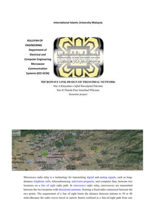
1. International Islamic University Malaysia
KULLIYAH OF
ENGINEERING
Department of
Electrical and
Computer Engineering
Microwave
Communication
Systems (ECE 6234)
MICROWAVE LINK DESIGN OF TRESSTRIAL NETWORK
Site A Khayaban e Iqbal Rawalpind Pakistan
Site B Thanda Pani Islambad PAkistan
Semester project
Student Name:-Syed Absar Kazmi
Matric No: G1220119
Phone number: 0182391572
Email address: engrabsarkazmi@gmail.com
Introduction
Microwave radio relay is a technology for transmitting digital and analog signals, such as long-
distance telephone calls, teleconferencing ,television programs, and computer data, between two
locations on a line of sight radio path. In microwave radio relay, microwaves are transmitted
between the two locations with directional antennas, forming a fixed radio connection between the
two points. The requirement of a line of sight limits the distance between stations to 30 or 40
miles.Because the radio waves travel in narrow beams confined to a line-of-sight path from one

2. antenna to the other , they don't interfere with other microwave equipment, and nearby microwave
links can use the same frequencies. Antennas used must be highly directional, these antennas are
installed in elevated locations such as large radio towers in order to be able to transmit across long
distances. Typical types of antenna used in radio relay link installations areparabolic antennas,
dielectric lens, and horn-reflector antennas, which have a diameter of up to 4 meters. For my case
am using 1.2m.Highly directive antennas permit an economical use of the available frequency
spectrum, despite long transmission distances.
Some of the basic briefing regarding to microwave link plan , budget and basic understanding ot
microwave link design including microwave spectrum , merits and short comings of point to point
links.
Microwave
Microwaves are shorter than radio waves with wavelengths measured in centimeters.
We use microwaves to cook food, transmit information, and in radar that helps to
predict the weather. Microwaves are useful in communication because they can
penetrate clouds, smoke, and light rain. The universe is filled with cosmic microwave
background radiation that scientists believe are clues to the origin of the universe they
call the Big Bang.
Communication (from Latin commūnicāre, meaning "to share”) is a purposeful activity of
exchanging information and meaning across space and time using various technical or natural
means, whichever is available or preferred.
Communication requires a sender, a message, a medium and a recipient, although the receiver
does not have to be present or aware of the sender's intent to communicate at the time of
communication; thus communication can occur across vast distances in time and space.
Communication requires that the communicating parties share an area of communicative
commonality. The communication process is complete once the receiver understands the sender's
message.
What is Microwave Communication
A communication system that utilizes the radio frequency band spanning 2 to 60 GHz.
As per IEEE, electromagnetic waves between 30 and 300 GHz are called millimeter waves
(MMW) instead of microwaves as their wavelengths are about 1 to 10mm.Small capacity systems
generally employ the frequencies less than 3 GHz while medium and large capacity systems
utilize frequencies ranging from 3 to 15 GHz. Frequencies > 15GHz are essentially used for short-
haul transmission.

3. Electromagnetic Spectrum
Electromagnetic waves are a form of energy waves that have both an electric and
magnetic field. Electromagnetic waves are different from mechanical waves in that
they can transmit energy and travel through a vacuum.
Electromagnetic waves are classified according to their frequency. The different types
of waves have different uses and functions in our everyday lives.
Figure . (1)
Merits of Microwave Radio
Significant advantages of microwave link towards fix-network media
 Less affected by natural calamities
 Less prone to accidental damage
 Links across mountains and rivers are more economically feasible
 Single point installation and maintenance

4.  Single point security
 They are quickly deployed
 Rapid installation
 Cost effective
 Low planning costs
 Insensitive towards unplanned disruptions
 High degree of flexibility as a result of being able to de-install and re-install at other location
Significant demerits of Microwave techbology towards line based media
 Limited transmission capacity
 Certain topographical conditions must be observed and require in certian circumstances the
erection of special structures (pylons)
 Relay stations necessary for long distances
 Disrupiton can be caused by weather
This section covers the basic technical elements that provide a foundation for understanding
line-of-sight radio frequency systems. The topics include:
 Frequency
 Wavelength
 Free-space Loss
 Precipitation Loss
 Antenna Gain
 Antenna Beam-width
 Transmit Power
 Multipath Interference
 Fresnel zones
 Effective Isotropic Radiated Power
 System Operating Margin
 Receive Signal Level
 Receiver Sensitivity
 Phase Relationships
 Multi-path Reflections
 Atmospheric Refraction
 Earth Bulge
 Signal-to-Noise Ratio
These elements must be clearly understood before attempting to undertake the design of a mission
critical line-of-sight microwave radio link.
Multipath Interference

5. When signals arrive at a remote antenna after being reflected off the ground or refracted back to
earth from the sky (sometimes called ducting), they will subtract (or add) to the main signal and
cause the received signal to be weaker (or stronger) throughout the day.
Signal-to-Noise Ratio
Signal-to-noise ratio (SNR) is the ratio (usually measured in dB) between the signal level received
and the noise floor level for that particular signal. The SNR is really the only thing receiver
demodulators really care about. Unless the noise floor is extremely high, the absolute level of the
signal or noise is not critical.
Figure 2 illustrates that weaker signals are larger negative numbers. It also graphically shows how
the SNR is computed.
Figure . (2)
Signal-to-
Noise Ratio
(SNR)
System
Operating
Margin
System
operating
margin (SOM)
is the difference (measured in dB) between the nominal signal level received at one end of a radio
link and the signal level required by that radio to assure that a packet of data is decoded without
error.
In other words, SOM is the difference between the signal received and the radio’s specified
receiver’s sensitivity. SOM is also referred to as link margin or fade margin.
Figure .
(3)System
Operating
Margin (SOM)
Effective
Isotropic
Radiated Power
Effective

6. isotropic radiated power (EIRP) is the actual RF power as measured in the main lobe (or focal
point) of an antenna. It is equal to the sum of the transmit power into the antenna (in dBm) added
to the dBi gain of the antenna. Since it is a power level, the result is measured in dBm.
Figure (4) shows how +24 dBm of power (250 mW) can be “boosted” to +48 dBm or 64 Watts of
radiated power.
Figure . (4) Effective Isotropic Radiated Power (EIRP)
Transmit Power
The transmit power is the RF power coming out of the antenna port of a transmitter. It is measured
in dBm, Watts or milliWatts and does not include the signal loss of the coax cable or the gain of
the antenna.
Receive Signal Level (RSL)
Receive signal level is the actual received signal level (usually measured in negative dBm)
presented to the antenna port of a radio receiver from a remote transmitter.
Receiver Sensitivity
Receiver sensitivity is the weakest RF signal level (usually measured in negative dBm) that a
radio needs receive in order to demodulate and decode a packet of data without errors.
3.1 Frequency

7. Frequency is measured in terms of the number of events in a given time duration. It is interesting
to note that low frequency sounds tend to propagate in a less directional manner than high
frequency sounds, as evidenced by the low frequency “boom, boom” we can hear (or feel) from a
high-powered audio system three cars away at a signal light. High frequency sounds tend to
propagate in a more directional or “line-of-sight” manner than lower frequencies, and they are,
therefore, attenuated to a larger degree by obstructions.
3.2 Wavelength
To be able to solve radio system engineering problems, you need to understand wavelength.
Wavelength is related to system frequencies and is an important factor in determining free space
loss, antenna gain, and Fresnel Zone boundaries—as well as the phase relationship between two
signals.
Electromagnetic waves propagate at the speed of light (in free-space or a vacuum), or
300,000,000 meters per second. As a result, wavelength in meters can be calculated by dividing
the number 300 by the frequency in MHz. To derive wavelength in inches, one can divide 11811
(the number of inches in 300 meters) by the frequency in MHz. From a practical standpoint, the
results of these formulae are approximate, since real-world electromagnetic waves propagate
through a medium, whether it’s the atmosphere, a conductor, or some other transmission medium.
Our atmosphere consists of numerous gases and water vapor, each of varying density. These
materials slow the propagation of radio waves to approximately 99.97% of their speed in a
vacuum or free space. Coaxial cable slows the signal down even more. For example, Times
Microwave LMR 400 coaxial cable, which is commonly used in RF antenna systems, has a
velocity factor of 85%. This means that the RF signal transmitted through that particular cable is
slowed to 85% of its free-space velocity.
3.3 Free Space Loss
Free space attenuation, commonly referred to as path loss, and is dependent upon the frequency of
the system involved and the length of the signal path. Free space attenuation (or loss) increases as
frequency goes up, for a given unit of distance. This occurs because higher frequencies have
shorter wavelengths, and to cover a given distance; they must complete many more cycles than
lower frequency signals, which have longer wavelength. During each cycle (wavelength) the
signals propagate, some of their energy is “spent.” Consequently, the higher the frequency (and
shorter the wavelength), the more rapidly the signals weaken as they propagate. Although the
formula for computing free space attenuation assumes signal propagation in a vacuum (outer
space), the attenuation through the atmosphere is reasonably similar.
The amount of free space attenuation can be computed using the following formula:
36.6 + 20 Log (F) + 20 Log (D)

8. Where:
F = Frequency in MHz
D = Distance in Miles
Example: A 2.4 GHz 5 mile path
Log (2400) = 3.380211 (x20) = 67.604225
Log (5) = 0.698970 (x20) = 13.979400
Path Loss = (36.6 + 67.604225 + 13.979400) = 118.183625 dB
3.4 Precipitation Loss
Frequency and wavelength are also affected by precipitation, which comes in many forms. The
detrimental effects of precipitation vary according to the physical properties of its form, as well as
its wavelength relationship to that of the particular frequency involved.
As explained earlier, wavelength is directly related to frequency, and one can determine the
approximate wavelength of a frequency in free space. To determine the wavelength in inches, we
simply divide 11811 by the frequency in MHz, as shown in the following calculations:
11811/5800 = 2.036, with ¼ wavelength then being approximately 0.509 inches.
11811/23000 = 0.514, with ¼ wavelength then being approximately 0.128 inches
Basically, when an object’s physical properties approach ¼ wavelength of a particular frequency,
they become highly reflective at that frequency. As shown in the two examples above, raindrops
can easily attain a dimension of 1/8 inch or more, effectively becoming multiple reflectors (or
more accurately stated, deflectors) in the path of a 23-GHz signal, while having much less impact
on a 5.8 GHz signal.
3.5 Antenna Gain
Antenna gain is directly related to frequency and the antenna signal-capture area. The number of
wavelengths in its signal-capture area determines gain of an antenna. Therefore, antenna gain will
go up in either of these two situations—if frequency goes up (allowing more, shorter wavelengths)
or if the size of signal-capture area goes up (also allowing more wavelengths).
Although there are many types of antennas, most point-to-point microwave systems utilize
parabolic antennas in order to achieve the required gain and reduce interference. The standard
formula for computing parabolic antenna gain assumes 55% illumination efficiency of the
antenna’s capture area. The term “illumination efficiency” refers to the percentage of power being
radiated by the source at the antenna’s focal point that illuminates the antenna reflector surface.
This formula is shown below.

9. 7.5 + 20 Log (F) + 20 Log (D)
A brief example will illustrates the antenna gain in further simpler form.
F = Frequency in GHz
D = Diameter in Feet
Example: A 2.4 GHz, 6 foot diameter, parabolic antenna
Log (2.4) = 0.380211 (x20) = 7.6
Log (6) = 0.778151 (x20) = 15.56
Parabolic Antenna Gain = (7.5 + 7.6 + 15.56) = 30.66 dBi
3.6 Antenna Beam-width
Antenna beam-width is another important antenna parameter, which is closely related to the
forward gain of an antenna. Since antenna gain results from redirecting available radiated energy
in a given direction, the higher the antenna gain of an antenna in its forward direction, the lower
its gain in other directions. That’s why larger antennas with higher gain are more directional.
Consequently, they are often used to solve interference problems when the interference source
may be located off-azimuth from the affected system path.
The beam-width of a parabolic antenna can be approximated with the following formula:
70/F x D
Where:
F = Frequency in GHz
D = Parabola diameter in feet
3.7 The Fresnel Zones
Creating “RF line-of-sight” for a microwave path requires more clearance over path obstructions
than is required to establish a visual “line-of-sight.” The extra clearance is needed to establish an
unobstructed propagation path boundary for the transmitted signal, based on its wavelength.
These boundaries are referred to as “Fresnel zones.” which are concentric areas surrounding the
direct path of the signal beam between the two antennas.
To establish “RF line-of-sight,” it is necessary to clear 60% of the 1st Fresnel zone boundary, from
the signal beam centerline outwards, across the entire signal path. Failure to do so will result in
additional signal loss caused by diffraction; the amount of loss will depend on the degree of
Fresnel zone encroachment.Although we are primarily concerned with clearing 60% of the 1
Fresnel zone radius to avoid signal diffraction loss, it is important to realize that Fresnel zones are

10. infinite in number. Each succeeding Fresnel zone has an exact ½ wavelength relationship to the
previous one, and the distance separating each Fresnel zone diminishes as the Fresnel zone
number increases.
These boundaries can be calculated with the following formula:
Where:
F1 = First Fresnel zone radius in feet
d1 = Distance from one end of path to reflection point in miles
d2 = Distance from reflection point to opposite end of path in miles
D = Total length of path in miles
f = Frequency in GHz
Figure . (5) Fresnel zone
3.8 Phase and Its Relationships
Phase can be described either in terms of degrees or radians (1 radian being approximately 57.3
degrees). A cyclede is fines as: an interval of time during which a sequence of a recurring
succession of events is completed.”
The drawing below represents one complete cycle, depicted in red, which is equivalent to 360
degrees—or one wavelength. If this drawing were extended, the next cycle would be identical to
the previous one, and so on. Phase can be used to identify the state of progress within a cycle.
Accordingly, one-half of a wavelength corresponds to 180 degrees of phase; one-quarter of a
wavelength corresponds to 90 degrees of phase; and so on. Phase relationships are important in
radio communications, since radio signals propagate through the atmosphere in analog form, with
an amplitude voltage that varies much like the drawing below, at the rate of the system frequency.

11. In the following example, however, the red and blue signals have a 180-degree phase (or
opposing) relationship with one another. This relationship frequently occurs in the case of a multi-
path reflected signal, causing the signals to cancel each other. The degree of signal cancellation
depends on the degree of phase opposition and the relative amplitude of the two signals.
Figure . (6)
Obviously, these illustrations present extreme cases, but the results always follow the same
principle. Just as in-phase vectors add, opposing ones subtract.
3.9 Multi-Path Reflections
Multi-path reflections occur when the reflection point for a given path has a reflective surface that
can be seen by both antennas. Multi-path reflected signals frequently cause problems in wireless
systems that have been implemented without proper path engineering. When people don’t
understand path engineering, they often believe that providing a “line-of-sight” path between the
two antennas is the only requirement. To avoid path obstructions, they simply install the antennas
as high as possible, hoping to overcome any obstacles, while avoiding the cost of system
engineering. Sometimes this approach works, but far more frequently, it produces systems with
unpredictable multi-path outages and susceptibility to interference from other systems in the area.
The path survey report is a very important part of the microwave system engineering, and is
prepared by the field engineer who carefully verifies and documents antenna coordinates, path
obstacles, terrain topology, and surface characteristics. The resulting report provides crucial
information that is required by the system engineer in order to perform reflection, link, and
reliability analysis of the system design.
3.10 The Reflected Signal
The nature of point-to-point terrestrial line-of-sight microwave systems causes most reflected
signals to occur at small angles, primarily due to the high ratio of path length versus antenna
height above a specific reflection point. This has the following negative effects:

12. 1. The antenna’s primary signal beam-width is usually broad enough to illuminate the reflection
point with the full signal power of the antenna’s primary beam.
2. Reflections occurring at small angles result in an inversion of the signal.
The following sketch depicts what occurs to a signal during the reflection process, as the reflected
signal becomes inverted. This results in a reflected signal that is 180 degrees out of phase with
respect to any direct path signal that has not been reflected.
Figure . (7)
3.11 Atmospheric Refraction
Earth is a living source of the gases, vapors, and water molecules that make up our atmosphere,
which decreases as it dissipates outward from the earth’s surface. Atmospheric content and
density varies significantly with local geophysical characteristics and time of day and season. The
only thing one can say for sure is that the atmosphere changes dynamically and is never constant.
Keep this principle in mind, as we discuss the effects of atmospheric refraction, which
significantly affects radio signal propagation.
These differences in propagation velocity result in refraction of a signal propagated through the
atmosphere, as shown in the following example.
Figure . (8)

13. In “normal” atmosphere near the earth’s surface, propagation velocity is approximately 99.997%
of that in free space. Under normal circumstances, atmospheric density decreases linearly with
altitude, resulting in a propagation velocity differential between the top and bottom of a wave
front. Since the upper part of the wave front propagates through less dense atmosphere than the
lower part to which it is coupled, it propagates faster than the lower part. The result is a signal
path that normally tends to follow earth curvature, but to a lesser to a degree. The bending of the
radio signal path caused by differences in atmospheric density is referred to as atmospheric
refraction.
“the K factor,is reffered as atmospheric refraction in microwave engineering, which describes the
type and amount of refraction.
Cases for K atmospheric refraction
A K factor of 1 describes a condition where there is no refraction of the signal, and it propagates
in a straight line.
A K factor of less than 1 describes a condition where the refracted signal path deviates from a
straight line, and it arcs in the direction opposite the earth curvature.
A K factor greater than 1 describes a condition where the refracted signal path deviates from a
straight line, and it arcs in the same direction as the earth curvature.
3.12 Physical Earth Bulge
Line-of-sight radio system engineering must deal with the effects of earth curvature, or Earth
Bulge. This term can reflect two different forms, so usage must be specific. The first form,
physical earth bulge,refers only to the effects of physical earth curvature. The second, “effective
earth bulge,” includes both the effects of physical earth curvature and the effects of atmospheric
refraction.
Earth bulge describes the effect of physical earth curvature along a direct path between two points
on the earth’s surface. The earth surface appears to “bulge upwards” in the path, with the peak of
the bulge occurring at mid-path.
In path profiling design you will see the addition of earth curvature to adjust the antenna
heights,the effects of physical “earth bulge” must be added to the terrain topology profile. The
amount of physical “earth bulge” along a path can be calculated from the following formula:

14. The data
3.13 Effective Earth Bulge
Effective earth bulge represents the effects of atmospheric refraction, or K, combined with
physical earth bulge. Any discussion of effective earth bulge must begin with an understanding of
the following rules. Otherwise, it is easy to become confused about K factors and earth bulge.
1. K factor represents the amount and type of atmospheric signal refraction.
2. A K factor of 1 represents the absence of any refraction effects and results in an “effective
earth bulge profile” that is identical to the “physical earth bulge profile.”
3. A K factor value other than 1 results in an “effective earth bulge profile” that differs from
the “physical earth bulge profile” by an amount equal to the atmospheric refraction effects.
Microwave signals propagated through normal atmospheric conditions do not travel in a straight-
line. Instead, they “normally” propagate in an arc with a radius approximately 1.33 (4/3) times
that of true earth radius. Therefore, we refer to this condition as K=4/3, or “normal earth.” This
refers to the amount of “earth bulge” that would normally result under these “standard”
atmospheric conditions. Because the signal arc of a propagated signal path through “normal
atmosphere” follows earth curvature, to a degree, this curvature effectively reduces the amount of
“earth bulge”—making it less than it is, when considered in strictly physical terms. When the
effects of atmospheric refraction are combined with “physical earth bulge,” a modified profile is
produced, known as “effective earth bulge.” Keep the following four rules in mind, since they are
true under all conditions.
When K=1, there is no refractive effect, and the signal path is a straight line. Under
1.these conditions “effective earth bulge” will be equal to “physical (or true) earth bulge.”
2. When K is less than 1, the refractive signal path arc is inverted (opposite) relative to physical
earth curvature, and “effective earth bulge” will be greater than “physical earth bulge.”
3. When K equals a number greater than 1, the refractive signal path is an arc in the same
direction as earth curvature, but may vary significantly from earth curvature,
thereby reducing “effective earth bulge” to something less than “physical earth bulge.”
4. When K = infinity, the refractive signal path arc follows earth curvature exactly, totally
canceling any “earth bulge” effect, making the earth appear “flat”. Since the propagated signal arc
follows earth curvature exactly regardless of path length, it can be stated that the relationship
between the two arcs remains constant for infinity.
5. When K = Negative, the refractive signal path is an arc that exceeds physical earth curvature
(beyond K = infinity), and effectively reverses the curvature of the earth with respect to the signal
path, making its surface appear like a “bowl”.

15. The following formula can be used to compute “effective earth bulge,” in feet, at any data point
in a path. It includes the effects of the applicable K factor:
Improving the Microwave System
 Hardware Redundancy
1. Hot standby protection
2. Multichannel and multiline protection
 Diversity Improvement
1. Space Diversity
2. Angle Diversity
3. Frequency Diversity
4. Crossband Diversity
5. Route Diversity
6. Hybrid Diversity
7. Media Diversity
MICROWAVE LINK DESIGN
The engineering of this system has to be tackled in a holistic way from site selection through to

16. the detailed design of a hop.The performance standard set has a dramatic impact on sytem
design.An attempt has been influence on the overall design simply to summarise the major
issues involved in achieving a cost effective high quality digital radiovsystem suitable for a
strategic utility environments. The initial phase of the system design involves a map study in order
to detennine the most likely connection DTM points of new sites into the network. The
(Digital Terrain Model) -A national database of pixel co-ordinates and corresponding average
pixel - is used in conjunction with some analysis altitudes
software in order to quickly ascertain whether the sites have “line-of-sight” clearence for the
given line with in that terrain range.
Microwave Link Design Process
The whole process is iterative and may go through many redesign phases before the required
quality and availability are achieved
Figure . (9)
Section A:
To design and generate the path profile , I will follow the procedure of Fully Linear Method the
steps needed:

17. 1. Coordinates of the transmitter site A
For the SITE A the transmitter is nominally plan as per aquisition survey to be at errected at
Khiyanban e Iqbal , Pirwadhai Rawalpindi Pakistan with the following coordinates:
Latitude: 33.635711°
Longitude: 73.039213°
Azmith angle: 83°
Altitude Sea Level (A.S.L): 508m
Picture
Figure . (10)
Coordinates of the reciever site B
For the SITE B the reciever is nominally plan as per aquisition survey to be at errected at Thanda
Pani Islamabad ,Pakistan with the following coordinates: in figure (11).
with the following coordinates:
Latitude: 33.654242°
Longitude: 73.220929°

18. Azmith angle:263°
Altitude Sea Level (A.S.L): 523 m
Figure . (11)
2. Transmitter and Receiver Separation:
The Transmitter and Receiver are 17 km apart. A straight line is drawn between
them as below:

19. Figure . (12)
2.1 Physical survey
Physical is necessary to verify the several parameters specifically the obsticles along
the path and the physibility of the link base on sites, towers and obstacles.Team
members are at both sites to make sure the clearence of link.
Tools required for surveys
1- mirror
2-GPS
3- Range finder
4-Compass
5-Binocouler
6-Camera
7-Walkie Talkie
Process to conduct line of sight survey
1- site cordinates
2- Azmith angle

20. 3- LOS conduction
Site cordinates
Site cordinates we can easily get by the map where our requirement is to deployed the
microwave link and it helps the team to reach that location by GPS
Azmith angle
In microwave link desgin as they are point ot point link so after planning the nominal
when it is to be surveid we are supposed to know the azimith angle to see the
obstacles physically on location fot that case I used software just by putting the values
of cordinates of both sides and elevation we can get the one azmith angle if angle is
less then 180 degree the other side member is supposed to see to first site with adding
angle achieved with addictional 180 deg so they can see each other or can have
several test to conducted to verfy LOS clearecne
Site A -B = 83 degree
By adding 180 degree ot this we cann achieved the other azmith
Site B- A = 263 degree
2.1.1 LOS conduction
Line of sght can be conducted by several mean based on site situation wether its new
site already established site.
1- Baloon test
2-Mirror test
3-terrain map software
4-physically moving along the path using GPS
After doing survey based on physically need to take the snaps as avidence to generate

21. report or on digital terrain map need to identify obstacles.
3. Obstacles Identification
The table below provides the data about obstacles along the path that should be taken into account
in the design process.
S/No Distance/Site A,
Khayaban-e-Iqbal (Km)
Altitude (m) On Ground (m) Nature
1 500 514 5 Town
2 570 509 3 Vegetation
3 800 500 0 Catarian Canal
4 1200 510 0 Catarian Canal
5 1.44 512 6 Town
6 2.31 517 5 Residence sector
7 3.1 524 12 Khana Plaza
8 5.18 517 5 Houses
9 6.18 485 0 Bharma canals
10 11 505 0 Open Land
11 13.5 535 5 Houses
12 14.100 538 4 Modern village
13 16.200 534 5 Modern village
Table . (1)
Table (1) shows the necessary data of obstacle along the path of path with different elevations
and distance from sita A and site B with their heights to make clearance margin in link.
4. Determination of Median value for K-Factor
The atmospheric refractivity for the worst month of atmosphere in Pakistan was obtained from
ITU-R.P.435.Then the surface refractivity is calculated using this formula:
With Next we use
the empirical
formula from technical note NBS-101[National Bureau of Standards, 1966] which connects / to
the surface refractivity :
For this case the K value
is assigned which is
given below
K = 2/3 =0.667

22. 5. Clearance Criteria
Recommendation ITU-R P.530 recommends using the following clearance criteria for climetic
region as Pakistan .The first Fresnel zone RF1 for the highest obstacle is obtained by:
The highest obstacle is located
at
d1 =14.100km from the transmitter
d2 = 2.900 km from the receiver.
The value of speed of light and frequency is given we can get lemmenda easily
C=3 x 108
F=14 GHz
Lemmeda = λ = C = 0.0214
f

23. Figure(13.1)
The radius of freznel zone can be computed once we get the values of lemmenda and d
RF1 = 7.174
Half power beam width gain an far field effective area for for frequency 14GHz and 1.2 m antenna
is given by following methametical model and simulator
Earth curvature = h = d1 x d2 where K = 2/3 = 0.667
12.75 x K
6. Path terrain from Site A to Site B particularly focusing on dominant obsticle throghout the
hope designated by A,B,C,D and E

24. Figure . (13)
Figure . (14)
Figure (14)show the overview of link in geo context software.
7. Figure show the Path profile with significant obstructions
Obstacles D1[km] D2[km] 0.6 x Rf1 Earth Curvature Total Height
A 0.500 16.50 1.933 0.98 2.913
B 5.18 11.82 4.009 7.199 11.208
C 13.5 3.5 3.522 5.550 9.072
D 14.100 2.90 3.276 4.808 8.084
E 16.200 0.80 1.844 1.523 3.367
Table . (1) Path profile data base
Table (1) presents the most prominent obsticles along the path of link and the distances of

25. obsticles from site A and site B,freznel zone clearence ,earth curvature and the total heights to take
counter measure to achieve the optimized link.
Figure . (15)
Figure (15) shows the obtacle B in google earth map along with the elevation profile which
provides a very obvious vision to terreain profile of the link to point out the obsticle to verify the
clearance margin.
Figure . (16)
Figure (16) shows the obtacle C in google earth map along with the elevation profile which
provides a very clear sight to terreain data which uses the STRM digital maps of the link to point

26. out the obsticle to identify and verify the clearence.
Figure . (17)
Figure (17 ) shows the obtacle D in google earth map along with the elevation profile which at 538
m elevation including the obsticle in modern village area provides a very obvious vision to
terreain profile of the link to point out the obsticle to verify the clearance margin.

27. Figure (17 a)
Figure . (17)
Figure (17) shows the obtacle E in front of side B wth elevation of 523 m in google earth map

28. along with the elevation profile which enhaces the visibility by the assistacne of software a very
clear analysis of terrain to achieve the clearance .
7. Antenna heights and reflection zone
The transmitter and receive antenna heights are computed by plotting the clearance margin and
earth curvature values from Table 2 for each critical point shown in figure (13) to achieve the final
elvation at antenna heights by considering two cases to investigate about reflection region .
Path Profile for SITE A to SITE B
The first Fresnel zone is derived from the transmit Site A situated at Rawalpindi,Pakistan with an
elevation of 508 m and the most prominent obstacle D with a total height of 8.084 m sum of
clearances summation with 542 m(elevation) to produce the 550.084 m. Yielding the following
Fresnel zone:

29. Figure . (18) Fresnel zone from Site A to B
From this figure(19) the height of the transmit antenna is 543 m (the reading from figure 18) -
508m (Site A elevation) = 35m and the height of receive antenna is 573m (the reading from figure
18) 523m (Site B elevation) = 50 m. However, the second Fresnel zone obtained from site B
located at Thanda Pani , Islamabad Pakistanis as follow:
Path Profile for SITE B to SITE A
Figure . (19) Fresnel zone from Site B to A
From this figure . (19) the height of the transmitter antenna is 593 m with 508m (Site A elevation)
= 85m and the height of receive antenna is 568m (the reading from figure 19) 523m (Site B
elevation) = 45m.

30. The complexity in this section is to choose the path profile design among both model these two
fisilibilities aforementioned. However, one of the solution among both will lead us to to select the
minimal refelctionn zonal link to be established as reflection is a major root cause of multipath
fading.
Figure . (20)Reflection point Nanogram
In path profile, I have defined the transmitter tower heights as hA for Site A and hB for the
receiver site B, and coomputing the ratio hA /hB , to take the corressponding values X axis .Figure
(20) On the y-axis two values of n are taken, the first for K= infinity and the second for
K=grazing. n1*D and n2*D from the shorter tower.
Case 1
For this case the ha antenna height is 35m and for the hB antenna height is 50m.By the given
formula the ration is computed to get the reflection area range.
hA = 35 = 0.7 Thus from figure (20) n1 , n2 and D1 , D2 are given below
hB 50
n1*D = 0.41 x 17km D1= 6.97 km
n2*D = 0.45 x 17 km D2= 7.65 km
This range from D1 to D2 and figure illustrates the range of reflection from Site A to Site B.

31. Reflection Zone
Figure . (21) Reflection zone from site A to B
Case 2
For this case the antenna height hB is 35m and for the hA antenna height is 50m.By the given
formula the ration is computed to get the reflection area range.
Case 2 = hA = 0.52
hB
n1*D = 0.34 x 17km D1= 5.78 km
n2*D = 0.42 x 17 km D2= 7.14

32. Reflection Zone
Figure ( 22) Reflection zone from site B to A
Ground reflections are the root cause of multipath fading. These reflections can be reduced or
rectified by adjustment of tower heights, effectively moving the reflection point from an area
along the path of greater reflectivity (such as a body of water) to one of lesser reflectivity (such as
an area of heavy forest) [1]. Consequently in my case I will choose the case 1 with a reflection
zone being in the Modern village area and a small reflection area compared to case 2 with a large
reflection zone in an open area. The average altitude of the zone of reflection being 73 m and the
altitude of the antennas known at the two ends, we can calculate the spacing of the interference
fringes using relation with the following values:
Space Diversity
In the case of space diversity, which is carried out in the vertical plane in line-of-sight links, the

33. spacing between the main and diversity antennas will thus have to be such that when on is located
in a zone of minimal field, the other is in a zone of maximum field; this condition is obtained
when the spacing between the antennas at station B, is equal to an odd multiple of the half half-
interference fringe
Case 1
F = GHz
D = path length in miles
Ht = height of antenna in in feets
= Diversity spacing at h2 end
Ht=h1 x d12
/2
H1= antenna height- reflection zone =543-485=58m
H1 in feets = 190.24
Antenna to reflection zone distance d1= 6.939
Now d1 in feets = 4.336 in miles
So ht = 190.24 x 4.3362
/2 = 1789 feets
= 2.2 x 103
x 10.625 = 0.9332 feet
14 x 1789
Case 2
= 1.3 x 103
x D
F x ht
= 0.5514
The above formention formulas gives the relation of spacing between antennas in order to ger the
optimize space diversity
station B antennas should be appart with 0.5514 as it obtained least among both cases so we
considered this as our solution to reflection as opmized link considring to derived spacing for
antennas as our site B area is open area is to overcome this issue we will deployed this technique
to prevent losses.

34. Figure ( 23)
Section 2
Using information from part 1, design a microwave link from site A to B such specification
 The availability is 99.999%,
 The transmitted power is 35dBm,
 The antenna is a parabolic dish with diameter 1.2 m, and 55% efficiency.
LINK BUDGET:
The link budget is the summation of all gains and losses in the radio communication link [4]. The
link margin can be computed by adding the transmit power in dBm(or dBw) with all of the
relevant link gains and losses in dB and then subtracting the required received signal level in
dBm(or dBw). The robustness of the link is then determined by the link margin. Links with small
margins are not likely to be very robust unless all of the gains and losses are very well understood
and modeled [5]. Some of the losses in a link budget are based on availability requirements, and
therefore the actual losses are not always exit . Availability requirements can drive some of the
fade margins that are included in the link budget. Therefore, losses that are frequently present
along the path such as the attenuation due to rain or other precipitation should be accounted in
order to ensure that the link is in fact available the required percentage of time. It is important that
the required fade margin be preserved if the true desired availability is going to be maintained.
Some of significant steps for the computation of link budget is as follow:
2.1- Effective Isotropic Radiated Power (EIRP)
The Effective Isotropic Radiated Power is the transmit power plus the antenna gain, subtracted
rest of loses like waveguide and/or radome losses.
EIRP [dB] = PTx [dBm] + GTx [dB] + Lwg [dB] + Lr[dBm]

35. EIRP =35dBm+42.32 dB-2dB - 1.5dB = 73.82 dB
The Power Transmitted is given by:
Where as ,
The operating frequency is 14 GHz, yields
GTx = 10 Log [0.55 x( Pi x 1.2 )2
= 42.32
0.0214
The transmitted power PTx = 35dBm
2.2- Free Space Loss
The free space loss model is shown below and can compute the value of FSL by the parameter of
frequency and distance
FSL = 32.45 + 20log (14000) + 20log(17)
FSL = 139.98

36. Figure .(24)
Knife Edge Diffraction Loss

37. Figure .(25)
2.3- Rain Attenuation
The link availability is 99.999%; the unavailability is then 0.001%. The rain fade exceeded 0.01%
must be calculated as reference using the ITU-R Rec. PN.530 model. Following steps needs to
consider to atain the rain attenuation parameter.
Step 1: The values of regression coefficients are o obtained using the recommendation ITU-
R P.838-3 with respect to the operating frequency. With
F = 14GHz, αV = 1.0646 and KV= 0.04126
Step 2: The value for the rain rate R(in mm/h) can be obtain using the Rec. ITU-R P.837-4, which
gives the rain rate. since the link is to be implemented in Pakistan therefore it should be the
same region which is K.
R = 20 mm/h
Step 3: the specific attenuation that gives the excess attenuation per kilometer is calculated as

38. follow:
= 0.04126 (20 )1.0646
Specific attenuation per kilometer = 1.001
Step 4: Computing the effective path length Deff . This is achieved by multiplying the actual path
length (in km) by a reduction factor r.
A first estimate to calculate r is given as
For R0.01<= 20 mm/hr ,
d0 = 35 e -0.015 x R0.01
, yields d0 = 25.9
Now by subtututing the values of do in r eqation can obtained the reduction parameter value.
r = 0.60
To obtained the effective path length the hope length should be multiplied with the reduction
factor and path length = 17 km
deff = d x r = 17 x 0.60
deff = 10.26
Step 5: Calculate the total path attenuation exceeded 0.01% of the time
A0.01= 1.001 x 10.26
A0.01 = 10.270 dB
Step 6: Attenuation exceeded for other percentages of time can calculated using the following
power law:
Ap = (.12 x .
001^-0.546+0.43 x
log (.001)) =10 log( 2.14 )= 3.30
A0.01

39. Ap = A0.01 + 3.30 = 10.270 +3.30 = 13.57
After manupulating all it is concluded that the attenuation at A0.001 = 13.57 dB
2.4-Atmospheric Absorption
Total absorption by atmospheric gases on a terrestrial radio link of length d is given
The specific attenuations due to
oxygen and water vapor can be obtained from the ITU-R Recommendation P.676 at a given
frequency. For our case with f=14 GHz,
Aa = 0.02 + 0.015 = 0.595 dB
2.5-Receiver Gain
The receiver gain is equal to the antenna gain less any radome loss, cable or waveguide
loss (receiver loss), polarization loss, and pointing loss.[6]
GR [dB] = GRX [dB] - LRadome [dB] - Lwg [dB] - Lpol [dB] - Lpt [dB]
GR [dB] = 42.32 -2-2 -0.2-1 =
The net received gain is then,
GR [dB]= 37.12
2.6. Unfaded Receive Signal Level (RSL):
In order to get unfaded RSL signal the reciever antenna gain and path loss will be subtracted from
the effective istropic radiated power.
RSL = EIRP _ PL - GRdb
RSL = 73.82 -139.98+37.12 = -29.04
2.7 Antenna Tilting

40. The Link Budget for the above is as follow:
Parameters SITE A SITE B
Latitude 33.635711° 33.654242°
Longitude 73.039213° 73.220929°
Frequency 14 GHz 14 GHz
Wavelength -0.0124 -0.0124
Antenna 1.2 m 1.2m
Parameters SITE A SITE B
Antenna Tilting 0.013 0.216
Polarization Vertical Vertical
Link Distance 17km 17km
Azmith Angle 83° 263°
Transmission Power 35dBm 35dBm
Transmission Loss -1.5dB -1.5dB
Transmission Antenna Gain 42.32 42.32

41. Radome Loss 2 2
EIRP 73.82 73.82
Path Loss (FSL) -139.98 -139.98
Transmission Pointing Error -1.0 dB -1.0 dB
RainLoss(99.999% availability) -12.59 dB -12.59 dB
Multipath -2.0dB -2.0dB
Atmospheric Loss 0.595 0.595
Total Path Losses -142.595 -142.595
Radome Loss -2 dB -2 dB
Receiver Antenna Gain 42.32dB 42.32dB
Polarization Loss -0.2dB -0.2dB
Receiver Loss -2dB -2dB
Receiver Pointing Error -1dB -1dB
Total Receiver Gain 37.12dB 37.12dB
Unfaded RSL -29.04 -29.04
Interference margin -1.0dB -1.0dB
Receiver Noise Figure 7dB 7dB
Noise Bandwidth 2.0 MHz 2.0 MHz
Total Noise Power -140.0dB -140.0dB
Unfaded Signal to Noise Ratio 104.19 104.19
Fademarginfor99.999%of time 40 40
C/N ratio 104.19 104.19
SD improvement factor 200.00 200.00
0.01% rain rate (mm/hr) 42.00 42.00
Threshold -80 -80
Net margin 24 24
Conclusion:
By going through all crtical analysis to verify the clearence for the first fresnel zone and by
maximum obstacle consideration to achieve the optimize antena heights takeing in consideration
relections.Space diversity is 1+0 due to open area.Once LOS report provides clearence margin
with all aspects the several parameters of link budgets are computed in order to get all parameters

42. which are emperical to systems some of the parameters are assumed based on pakistan’s
functional link budgets and tried to assume purely nearest assumptions to achieve realistic
values.In pakistan the antenna heights standard are 30.35.45.65,and 85 so need to decide within
this range as per fisibilities.For calculations standard formulas and softwares are used to compute
all parameters. The availibility is considered as 99.999% time availability would require a 40-dB
margin. This depict us that with the minimum unfaded C/N for the link calculated as 104
dB, the link would require104dB+40dB or a C/N=144 dB (unfaded) to meet the objective of
99.999% time availabilityPermitting the validation of the pure Rayleigh assumption, the
unavailability of the link is 1-0.99999 or 0.00001. A year has 8760 h or 8760x60 min. Ultimately
the total time for the year is 8760 hrs and in mins it will be 525600 minites so compute the outage
it will be C/N would be less than 104dB would be 0.00001x8760x60 or 5.256 min.
References:

43. Radio System Design for Telecommunication, Third Edition Roger L. Freeman, p48.
Microwave Engineering Land & Space Radiocommunications Gérard Barué p169.
Microwave Engineering Land & Space Radiocommunications Gérard Barué p190.
Seybold J.S. Introduction to RF Propagation 2005, p79
Fundamentals of Radio Link Engineering
© 1999 J. Frank Jimenez
Planning a Microwave Radio Link , By Michael F. Young President and CTO ,YDI Wireless
An introduction to link desgin by SAF
ITU-R recommendations
www.googleearth.com
For elevation and obstacles identifcation
www.Geocontext.com
To make path profile as per our planned sites
www.rankstel.com
www.isitwireless.com
www.n9zia.ampr.org/distance.main.cgi
www.n9zia.ampr.org/tilt.cgi