Sub-Saharan-African-Eurobond-yields--What-really-mat_2018_Review-of-Developm.pdf

1. Available online at www.sciencedirect.com
ScienceDirect
HOSTED BY
Review of Development Finance 8 (2018) 49–62
Sub-Saharan African Eurobond yields: What really matters beyond global
factors?夽
Christian Sengaa,∗, Danny Cassimona, Dennis Essersa,b
a Institute of Development Policy (IOB), University of Antwerp, Belgium
b Economics and Research Department, National Bank of Belgium, Belgium
Available online 24 May 2018
Abstract
This study explores the drivers of secondary market yields of Sub-Saharan African (SSA) sovereign Eurobonds from 2008 to mid-2017. Our
results indicate that, beyond global ‘push’ factors, country-specific ‘pull’ factors such as inflation and GDP growth matter too for SSA Eurobond
performance. A panel error-correction analysis suggests large heterogeneity in the short-term influence of our global and country variables across
countries. We find no significant effect of bond-specific factors on yields when push and pull factors are accounted for. By emphasizing the
prominence of country variables, reflecting the quality of countries’ macroeconomic management and their economic performance, our results
qualify the common view that SSA countries have little control over their market borrowing costs.
© 2018 Africagrowth Institute. Production and hosting by Elsevier B.V. This is an open access article under the CC BY-NC-ND license
(http://creativecommons.org/licenses/by-nc-nd/4.0/).
JEL classification: F34; G15; H63
Keywords: Public debt; International bonds; Bond yields; Sub-Saharan Africa
1. Introduction
During the 1980s and 1990s many Sub-Saharan African
(SSA) countries saw an unsustainable build-up of external pub-
lic debt, due to a toxic combination of commodity boom-bust
cycles, easy lending by official creditors and international banks,
bad domestic policy and, in some cases, civil war (Brooks et al.,
1998; Easterly, 2002; Thomas and Giugale, 2015). Debt relief
by creditors was initially limited to non-concessional reschedul-
ings, allowing debtor countries only to postpone repayment.
夽 Funding: This work was financially supported by the Academic Research
Organisation for Policy Support (ACROPOLIS) initiative of the Belgian Devel-
opment Cooperation (DGD) in the framework of the Belgian policy research
group on Financing for Development (BeFinD) consortium. We are grateful for
the comments received from participants in the 2017 CSAE Annual Conference
in Oxford. The views expressed in this paper, as well as any remaining errors,
are those of the authors only and should not be ascribed to DGD, the National
Bank of Belgium, or the Eurosystem.
∗ Corresponding author.
E-mail addresses: christian.senga@uantwerpen.be (C. Senga),
danny.cassimon@uantwerpen.be (D. Cassimon), dennis.essers@uantwerpen.be
(D. Essers).
Gradually, however, it was acknowledged that debt problems
transcended temporary liquidity concerns and more extensive
debt service and debt stock relief was granted (Cassimon and
Essers, 2017). A watershed event was the 1996 Heavily Indebted
Poor Countries (HIPC) initiative which aimed at reducing even
the worst debt burdens to manageable levels, subject to policy
reforms. The HIPC initiative was later deepened and comple-
mented with the Multilateral Debt Relief Initiative (MDRI) in
2005 to result in well over US$100 billion of debt cancellation
for 30 SSA countries. Merotto et al. (2015) show that the public
debt to GDP ratio of the average SSA HIPC came down from
over 100% prior to HIPC decision points to below 30% just
after HIPC/MDRI completion. Also a number of non-HIPCs,
most notably Nigeria, have enjoyed large debt relief (Dijkstra,
2013).
Faced with huge infrastructure and other needs, SSA coun-
tries have been filling up again the ‘clean slates’ debt relief
provided them with by borrowing from a wide range of domestic
and external creditors (Prizzon and Mustapha, 2014; Cassimon
et al., 2015; Merotto et al., 2015). This paper looks at one chan-
nel of external borrowing by SSA sovereigns that has attracted
relatively much attention from policymakers, i.e., the issuance
https://doi.org/10.1016/j.rdf.2018.05.005
1879-9337/© 2018 Africagrowth Institute. Production and hosting by Elsevier B.V. This is an open access article under the CC BY-NC-ND license
(http://creativecommons.org/licenses/by-nc-nd/4.0/).

2. 50 C. Senga et al. / Review of Development Finance 8 (2018) 49–62
of international bonds in the Eurodollar market (henceforth:
Eurobonds) (Mecagni et al., 2014; UNCTAD, 2016).1
Starting in 2006, no less than 16 SSA governments (exclud-
ing South Africa) have issued Eurobonds, most of them for the
first time ever, in what te Velde (2014) has called a ‘beauty con-
test’. Taken together, they have raised about US$29 billion in 35
issuances between September 2006 and June 2017.2 Notwith-
standing potential benefits from debt diversification, Eurobond
issuance holds a number of risks for SSA countries. First of
all, the US dollar denomination of these bonds exposes their
issuers to exchange rate risks. Because the required princi-
pal repayments are concentrated, typically in a single ‘bullet’
installment, Eurobonds also involve greater redemption risks
than amortizing loans. In contrast to the syndicated bank loans
that dominated the commercial debt of African countries during
the 1980s, Eurobonds are marked by a much more diffused and
diverse set of creditors (Bertin, 2016). Moreover, it is widely
believed that investor appetite for SSA bonds has been fueled
by record-low interest rates in advanced economies and com-
modity price recovery in the aftermath of the global financial
crisis, trends that have now reversed or could reverse in the near
future (Masetti, 2015; Standard and Poor’s, 2015; Sy, 2015).
Indeed, a recent study by Presbitero et al. (2016) finds that
low-income developing countries are more likely to issue inter-
national bonds when US interest rates are low and commodity
prices high, particularly so for SSA sovereigns, and that issuance
occurs at higher spreads in times of market uncertainty. But next
to global factors, domestic fundamentals seem to matter too at
issuance. Presbitero et al. (2016) show that low-income coun-
tries’propensitytoissueEurobondsriseswitheconomicsizeand
development, lower external debt and higher government effec-
tiveness, and that issue spreads are lower for countries with a
stronger current account balance, lower public debt, faster eco-
nomic growth and an effective government. Olabisi and Stein
(2015) demonstrate that, even after controlling for such global
and domestic variables, SSA sovereigns pay a premium on their
bonds at the moment of issuance, relative to other regions.
This paper takes the analysis of SSA Eurobonds beyond the
primary market by studying the drivers of the secondary market
yields of these bonds. Whereas changes in secondary market
yields have no immediate impact on the interest costs of exist-
ing fixed-rate securities, they do reflect the marginal cost of
new borrowing through similar instruments. Concentrating on
secondary market yields allows one to exploit important within-
country variation, a dimension which is typically very limited
in the primary market. It should therefore not come as a sur-
prise that most of the literature on emerging market borrowing
takes secondary rather than primary market yields/spreads as the
object of study. Given our focus on SSA, where most countries
1 The term ‘Eurobond’ generally refers to an international bond denominated
in a currency other than that of the issuer or of the place where it is issued. In
parallel to issuing Eurobonds, SSA countries have also begun to develop their
domestic bond markets. For more details, see Dafe et al. (2018), Essers et al.
(2016), Berensmann et al. (2015) and Mu et al. (2013).
2 Not all of this constituted additional funds, however, as some bonds were
(partly) issued to roll-over or exchange older debt titles.
have so far issued only a few bonds each (usually separated by
multiple years), the choice for secondary market yields makes
much sense, we believe.
Apart from Senga and Cassimon (2018) who investi-
gate spillover effects among SSA Eurobonds, Gevorkyan and
Kvangraven (2016) is, to the best of our knowledge, the only
paper to date that attempts to explain the variation in the sec-
ondary market yields of a larger set of SSA Eurobonds.3 With
monthly data for nine countries (Republic of Congo, Côte
d’Ivoire, Gabon, Ghana, Namibia, Nigeria, Rwanda, Senegal
and Zambia) over December 2007 – February 2014, the authors
find that yields in SSA are driven by commodity prices, global
financial market uncertainty and US interest rates. We build and
improve upon Gevorkyan and Kvangraven (2016) in several
ways. First of all, we extend the sample to 14 countries, dis-
carding the Republic of Congo and adding Angola, Cameroon,
Ethiopia, Kenya, Mozambique and Tanzania, and update the
time span to June 2017, thereby incorporating the latest oil price
bust and recovery, and the start of monetary policy tightening
by the US Federal Reserve. Second, next to global factors, we
include in our empirical models a broad set of country-level vari-
ables, such as international reserves, public debt, GDP growth
and inflation. Except for reserves, these variables are absent from
the analysis by Gevorkyan and Kvangraven (2016). Including
domestic macroeconomic fundamentals enables us to capture
the domestic ‘pull’ factors that may drive SSA Eurbond yields,
besides common international ‘push’ factors. Where possible,
we also examine the influence on yields of bond-specific charac-
teristics; among other, the size and maturity of individual bonds,
the redemption schedule, and whether or not proceeds are used to
fundinfrastructure.Toevaluatetherelativeimportanceofglobal,
domestic and bond-specific variables more formally, we per-
form a dominance analysis using the methodology of Azen and
Budescu (2003). Third, relative to Gevorkyan and Kvangraven
(2016), this paper employs a larger variety of estimators, in line
with key studies in the emerging market bond spreads literature
(see e.g., Dailami et al., 2008; Gonzalez-Rozada and Yeyati,
2008; Bellas et al., 2010; Kennedy and Palerm, 2014). To dis-
tinguish between long- and short-run dynamics, we formulate a
panel error-correction model, which we estimate with the Pooled
Mean Group (PMG) estimator of Pesaran et al. (1999).
To preview our main conclusions, we find that, beyond global
push factors, country-specific pull variables, including infla-
tion and GDP growth, also affect SSA Eurobond yields. Our
panel error-correction results suggest large heterogeneity in the
short-term influence of global and country explanatory vari-
ables across countries. Bond-specific factors such as bond size
and maturity generally enter our regressions with the expected
signs but are not statistically significant once global and coun-
try variables are taken into account. The importance of country
variables as drivers of yield is confirmed by our dominance
analysis. Hence, the common view that market borrowing costs
3 Some other studies have incorporated a handful of SSA countries in their
bond samples, usually as constituents of the JP Morgan Emerging Market Bond
Index (EMBI) Plus or Global.

3. C. Senga et al. / Review of Development Finance 8 (2018) 49–62 51
are outside the span of control of SSA countries needs to be
qualified.
The remainder of the paper is structured as follows. Section 2
summarizes the relevant literature on emerging and developing
country bond yields/spreads. Section 3 describes our SSA sam-
ple and outlines the estimation strategy. Our results are presented
and discussed in Section 4. Section 5 concludes.
2. Literature review
We look into the existing literature on emerging market bond
yields to inform our choice of global factors and country fun-
damentals to be considered as determinants of SSA sovereign
bond yields. For instance, Hong-Ghi et al. (2003) distinguish
three categories of variables in their study on emerging market
bond spreads, i.e., liquidity and solvency variables, macroeco-
nomic fundamentals, and external shocks. In the first category
they group variables such as exports, imports, ratios of debt
and foreign reserves to GDP, GDP growth, the current account
balance, and the debt service to export ratio. The second cate-
gory is made up of variables such as inflation (as a proxy of the
quality of macroeconomic management), the terms of trade, and
the real exchange rate. Finally, US Treasury bill rates and the
real oil price are considered as external shocks. The results of
Hong-Ghi et al. (2003) indicate that, taken together, liquidity and
solvency variables and fundamentals explain most of the spread
variations in the 11 emerging market economies they consider
during the 1990s. Changes in the US interest rate too appear to
affect emerging market spreads. Similar variable categorizations
have been used by other studies and their results converge to the
importance of some or all of the above variables in determining
bond yields and/or spreads (see e.g., Haque et al., 1996; Genberg
and Sulstarova, 2008; Jaramillo and Tejada, 2011; Maltritz et al.,
2012; Jahjah et al., 2013; Maltritz and Molchanov, 2013, 2014).
Other, related literature elaborates on the factors affecting
capital flows between advanced and emerging economies. With
theLucasparadox4 havingbeenempiricallyinvalidatedinrecent
studies (Reinhardt et al., 2013), most researchers now agree that
capital flows are driven by both ‘push’ factors that emanate from
the countries where lenders reside and ‘pull’ factors originat-
ing in the borrowing countries (Fratzscher, 2012; Suttle et al.,
2013; Gueye and Sy, 2015). A simple but intuitive descrip-
tion of these factors is provided by Suttle et al. (2013), who
refer to very loose monetary policy and the prospect of low
returns in advanced economies, and higher growth and interest
rates in emerging markets as respectively push and pull factors
driving the flow of capital between these economies. A more
comprehensive view is adopted by Fratzscher (2012). He takes
an international diversification perspective and considers com-
mon shocks as push factors, and idiosyncratic, country-specific
determinants as pull factors in his analysis on the drivers of cap-
ital flows from 2005 to 2010. He argues that push factors were
4 The Lucas paradox or the Lucas puzzle is the observation that capital does
not flow from developed countries to developing countries despite the fact that
developing countries have lower levels of capital per worker (Lucas, 1990).
the most important drivers of net capital flows in 2005-2007
and during the 2007-2008 global financial crisis, while pull fac-
tors dominate in explaining capital flows to emerging market
economies in the recovery period thereafter. A similar view is
also taken by Gueye and Sy (2015), who estimate the cost of bor-
rowing by African countries from a model including prevailing
push and pull factors.
Interestingly, the foregoing frameworks allow to test the
market discipline hypothesis, since the significance of macroe-
conomic fundamentals (pull factors) can be interpreted as
evidence of markets’ ability to discriminate between countries
based on their respective economic performance. For example,
Bellas et al. (2010) find that fundamentals influence emerging
market bond spreads in the long run while financial market
volatility is only important in the short run using data on 14
JPMorgan Emerging Market Bond Index (EMBI) constituents
from 1997 to 2009. Dailami et al. (2008) consider 17 EMBI
countries from 1991 to 2004 and their results indicate a signif-
icant, non-linear impact of US interest rate policy on emerging
market bond spreads, with countries having moderate debt levels
suffering less from increases in US interest rates.
Besides push and pull factors, a notable study by Feyen et al.
(2015) sheds light on the importance of bond-specific charac-
teristics in the determination of international bond yields of
emerging and developing economies on the primary market (i.e.,
at issuance). Using a sample of 71 countries over 2000–2014
and controlling for global and country-level factors, Feyen et al.
(2015) find a statistically significant positive impact of bond
maturity on primary market yields, but no independent effect of
bond size.
Also the relatively recent move of SSA countries into inter-
national markets has caught the interest of researchers and
policymakers. Sy (2013) believes that the record-low interest
rates in the US and other advanced economies are the main
(push) motive for investors’ purchases of SSA Eurobonds. On
the pull side, he cites promising GDP growth supported by
stronger policy frameworks, improved governance, and sharply
reduced debt burdens. However, Sy (2013) draws a pessimist
picture of the sustainability of SSA Eurobonds as, according to
him, none of these push or pull factors are expected to continue
over the mid to longer term, given, for example, monetary policy
normalization in advanced economies.
As mentioned above, our analysis complements the work
of Gevorkyan and Kvangraven (2016) by extending the sam-
ple of SSA sovereign bonds to more countries, and to more
than one bond issue per country when available. Along with
this extension, we increase the number of country fundamentals
that are considered and distinguish between short- and long-run
dynamics in our assessment of the association of global and
country-specific factors with bond yields. We also carry out an
analysis at the individual bond level to assess the significance of
bond-specific characteristics in affecting yields.

4. 52 C. Senga et al. / Review of Development Finance 8 (2018) 49–62
3. Methodology and data
3.1. Empirical model specification
ToempiricallyinvestigatethedriversofSSAEurobondyields
in secondary markets, we follow the emerging market bond
spreads literature and start with a basic formulation of the long-
run relationship between yields, global push factors and country
fundamentals/domestic pulls:
yit = αi +
J
j=1
βjGLOBjt +
K
k=1
γkDOMkit + εit (1)
where yit are the log Eurobond yields of country i at time t;
GLOB and DOM are vectors of, respectively, J global and K
domestic variables; β and γ are sets of slope parameters assumed
to be the same for all countries; αi is an intercept that may vary
across countries; and εit are well-behaved error terms. This static
model can be estimated using simple pooled OLS (POLS), the
random effects (RE) estimator, or fixed effects (FE), depending
on the assumptions one makes with respect to αi. In addition,
limiting ourselves to bonds with sufficiently long yield series we
can apply Mean Group (MG) estimation, which averages panel-
specific coefficients estimated using OLS (Pesaran and Smith,
1995).
Since yields are expected to depend on their own lags and on
lags of the independent variables, it makes sense to also consider
a more dynamic specification. Taking heterogeneous parameters
we can reformulate the model as:
yit = δi + ηiyit−1 +
J
j=1
θ1jiGLOBjt +
J
j=1
θ2jiGLOBjt−1
+
K
k=1
λ1kiDOMkit +
K
k=1
λ2kiDOMkit−1 + vit.
(2)
After rearranging we obtain the following panel error-
correction representation:
yit = φi[yit−1 − αi −
J
j=1
βjiGLOBjt −
K
k=1
γkiDOMkit]
−
J
j=1
θ2ji GLOBjt −
K
k=1
λ2ki DOMkit + vit
(3)
where φi = (ηi − 1); αi = δi
1−ηi
; βji =
θ1ji+θ2ji
1−ηi
; and γki =
λ1ki+λ2ki
1−ηi
. The expression in square brackets is the gap between
lagged yields and the determinants of their equilibrium levels,
with βji and γki the long-run (semi-)elasticities of the variables
included in, respectively, GLOBj and DOMk for country i (cf.
Eq. (1)). The coefficients θ2ji and λ2ki represent the short-run
reactions to shocks in global and domestic variables. And error-
correction term φi captures the speed at which countries’ bond
yields will return to their long-run equilibrium (steady state)
after such shocks.
There are again different ways to estimate Eq. (3). First, one
can impose homogeneity in all parameters, except intercepts,
and estimate a dynamic FE model. Alternatively, one could again
fall back on the estimation of separate regressions for each panel
(country)andthenexaminetheaveragesofallcoefficientsacross
panels, i.e., the MG estimator. We prefer the intermediate Pooled
Mean Group (PMG) estimator, first proposed by Pesaran et al.
(1999), which constrains the long-run parameters to be common
across panels (βji=βj and γki=γk), but allows for panel-specific
error-correction terms and other short-run parameters.5
The PMG approach has intuitive appeal for our purposes and
has featured in key studies on emerging market bond spreads
(Dailami et al., 2008; Bellas et al., 2010; Kennedy and Palerm,
2014). As noted in those studies, it can be plausibly argued that
in the long run financial markets hold economies to the same
standards, while in the short run market perceptions of countries’
creditworthiness may react differently to similar shocks (be it in
global or country variables).
In separate regressions, we also investigate the marginal
influence of bond-specific characteristics on secondary market
yields, a dimension which is all but absent from the literature on
emerging and frontier market bonds (with the notable exception
of Feyen et al. (2015), which only considers yields at the time
of issuance). More specifically, we extend specification (1) as
follows:
yit = αi +
J
j=1
βjGLOBjt +
K
k=1
γkDOMkit
+
L
l=1
μlBONDlbi + ωbit (4)
where BONDl is a vector of L bond-specific factors for bond
b of country i. Since all bond characteristics we consider are
time-invariant, we cannot include bond fixed effects. However,
the inclusion of country fixed effects αi in Eq. (4) helps us
separate the influence of bond factors from country-specific
attributes in countries that have issued multiple bonds. We
also use this equation to perform a dominance analysis in the
spirit of Azen and Budescu (2003), whereby the respective
explanatory power of our exogenous variables is assessed. More
specifically, the general dominance of one (or set of) indepen-
dent variable(s) over other regressors is determined based on a
comparison of dominance statistics, computed as the weighted
averagemarginalcontributiontotheoverallfitstatisticthatan(or
set of) independent variable(s) makes across all models in which
it is included.6 Such a dominance analysis further clarifies the
relative importance of global, country-specific and bond-level
factors in explaining the evolution of SSA Eurobond yields.
5 It is well known that, because of the correlation between the lagged depen-
dent variable and the error term, all three estimators will show bias, which
diminishes with longer time series (Nickell, 1981). Since the time dimension of
our sample dominates the cross-sectional dimension we assume that our series
are long enough to mitigate this dynamic panel bias (Gonzalez-Rozada and
Yeyati, 2008).
6 For a more detailed discussion of the dominance analysis, see Budescu
(1993) and Azen and Budescu (2003).

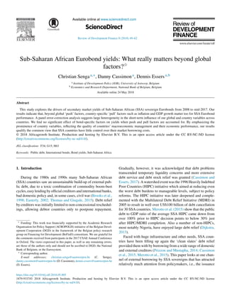
5. C. Senga et al. / Review of Development Finance 8 (2018) 49–62 53
3.2. Our dataset
We have been able to collect secondary market yields-to-
maturity for 31 sovereign Eurobonds of 14 SSA countries from
Thomson Reuters Datastream (see Appendix Table A.1). This
covers the near-universe of non-South African SSA sovereign
Eurobonds issued between September 2006 and September
2016.7 For our first set of yield regressions, in which we focus
on the role of global push versus country pull factors and leave
aside bond specifics, we limit ourselves to one bond per country,
so as to better balance the sample in terms of country observa-
tions. In case a country has issued multiple bonds, we select
for each country the bond with the longest yield series (typ-
ically countries’ debut bonds), in order to maximize the time
dimension of our estimation. After averaging Eurobond yields
at monthly frequency between January 2008 and June 2017, we
end up with an unbalanced panel dataset of 14 countries/bonds
and 795 observations in total. When estimating Eq. (4), which
includes bond characteristics, we make use of the whole sample
of 31 SSA Eurobonds, considering multiple issues per country
where available.
We follow the literature and take the Bloomberg Commod-
ity Index, the VIX and yields on 10-year US Treasury bonds to
capture the influence of, respectively, global commodity prices,
market volatility and liquidity/monetary conditions, i.e., the
push factors in our model. As pull factors, we select the follow-
ing macroeconomic fundamentals: the current account balance,
government debt, primary fiscal balance, foreign reserves, GDP
growth, exchange rate changes, and inflation. All country vari-
ables have been collected at their highest available frequencies
and interpolated to monthly frequency where needed. Appendix
Table A.2 provides the exact definitions and original sources of
our variables.
As concerns bond characteristics, we have constructed (time-
invariant) dummies to distinguish between bonds involving a
single bullet redemption of the principal and bonds with some
amortization; debut and non-debut bonds; bonds with different
sizes (below, equal to, or above US$1 billion) and original matu-
rities (less than, equal to, or more than 10 years); and whether or
not the stated use of proceeds (explicitly) includes an infrastruc-
ture component. The rationale for including the infrastructure
bond dummy is that infrastructure investments are easier to mon-
itor by international investors and may start generating returns
earlier than, say, investments in education or health. This could
instill relatively more trust in infrastructure bonds. All infor-
7 To ensure a minimum time series dimension for yields, we do not include
more recently issued SSA Eurobonds. Bonds for which no or insufficient yield
data could be retrieved from Datastream are the 2006 and 2010 issues of the
Seychelles, the 2007 issue of the Republic of Congo, and the 2010 issue of Côte
d’Ivoire. We do include in our sample a number of bonds that are, strictly speak-
ing, not ‘sovereign Eurobonds’ but have similar characteristics: Angola’s 2012
loan participation notes issued by Northern Lights III, a special purpose vehicle
backed by Russian bank VTB Capital, but with the Angolan government as the
ultimate guarantor; Mozambique’s 2013 government-guaranteed bond, issued
by state-owned tuna fishing company Ematum; and the Tanzanian government’s
2013 privately placed floating rate notes.
Fig. 1. Evolution of yields of selected SSA Eurobonds.
Fig. 2. Boxplots of SSA Eurobond yields.
mation on bond characteristics was sourced from the original
prospectus documents.8
Figs. 1 and Figure 2 show the evolution and dispersion of SSA
Eurobond yields. It is clear that these yields do tend the follow
similar trends, but also that there is quite some heterogeneity
between bonds/countries. Whereas most yields are found in the
5–10% range, within-bond yield variation is substantial. Bonds
like those of Ghana, Zambia and Mozambique have seen yields
exceeding 15% at times. Mozambique in particular appears to
be an outlier in terms of Eurobond yields. This may not come
as a surprise, given the scandals that have developed around
Mozambique’s bonds (and a set of other, undisclosed loans) and
the country’s ultimate default early 2017 (Hanlon, 2016; IMF,
2018). We take the special case of Mozambique into account
when testing the robustness of our econometric results. Sum-
8 For example, in the prospectus of the 2013 Eurobond of Gabon one can
read: “The net proceeds of the Offered Notes will be used to accelerate and sup-
port the infrastructure projects identified by the Schéma directeur national des
infrastructures, including the development of the bypass road in the Owendo
zone, the development of electricity generation and transmission, in particular
the Chutes de l’Impératrice dam, the finalisation of the Libreville-Franceville
road and the South and South-West corridors”. Conversely, the prospectus
of the 2011 Nigerian Eurobond states: “The net proceeds of the issue, after
payment of commissions and expenses, will be used for general budgetary pur-
poses”. Accordingly, we classify the first (second) bond as an infrastructure
(non-infrastructure) bond.

6. 54 C. Senga et al. / Review of Development Finance 8 (2018) 49–62
Table 1
Summary statistics of global and country variables.
Variable Obs. Mean Std. Dev. Min Max
SSA Eurobond yield (YIELD) 1255 0.073 0.026 0.032 0.253
Bloomberg commodity index (BCOM) 3385 374.036 65.539 235.59 509.133
VIX 3385 0.222 0.079 0.124 0.563
10-year US Treasury bond yield (USTB) 3385 0.026 0.007 0.015 0.040
Current account balance to GDP (CABAL) 3385 0.181 6.038 −15.763 29.154
Government gross debt to GDP (DEBT) 3385 36.900 18.126 7.276 115.2
Government fiscal balance to GDP (FISCBAL) 3385 −1.639 3.698 −9.642 12.642
Foreign reserves to GDP (RES) 3385 10.629 6.067 0.016 31.037
GDP growth (GDPGR) 3385 0.004 0.011 −0.026 0.034
Exchange rate change (XRTCH) 3385 0.007 0.036 −0.194 0.350
Inflation (INFL) 3385 0.007 0.008 −0.043 0.098
Log SSA Eurobond yield (LYIELD) 1255 −2.674 0.314 −3.442 −1.373
Log Bloomberg commodity index (LBCOM) 3385 5.908 0.182 5.462 6.233
Log VIX (LVIX) 3385 −1.557 0.307 −2.086 −0.575
Log 10-year US Treasury bond yield (LUSTB) 3385 −3.689 0.283 −4.230 −3.210
Notes: For variable definitions and sources, see Appendix Table A.2.
Table 2
Pairwise correlations between yields and main explanatory variables.
LYIELD LBCOM LVIX LUSTB CABAL DEBT FISCBAL RES GDPGR XRTCH INFL
LYIELD 1.0000
LBCOM −0.4570* 1.0000
LVIX 0.2633* −0.3070* 1.0000
LUSTB −0.0188 0.0417* 0.3266* 1.0000
CABAL −0.3074* 0.1418* 0.1775* 0.1644* 1.0000
DEBT 0.5246* −0.1781* −0.3108* −0.2676* −0.4892* 1.0000
FISCBAL −0.1662* −0.0142 0.1995* 0.1390* 0.4309* −0.3007* 1.0000
RES −0.0142 0.0692* −0.0328 0.0147 0.2198* −0.1442* 0.2479* 1.0000
GDPGR −0.1551* 0.4007* 0.0942* 0.2575* 0.2050* −0.1618* 0.0823* 0.0540* 1.0000
XRTCH 0.0687* −0.0869* 0.0748* −0.0363* −0.0563* 0.0355* −0.0659* −0.0270 −0.1071* 1.0000
INFL 0.3039* −0.0264 0.0034 0.0875* −0.0257 0.0987* −0.1147* 0.1996* −0.0032 0.1001* 1.0000
Notes: For variable definitions and sources, see Appendix Table A.2.
* Significant at 5% level.
mary statistics and pairwise correlations between (log) yields
and the above-described global and country-level variables are
presented in Tables 1 and Table 2. Yields correlate positively
with the VIX, debt to GDP ratio, exchange rate depreciation,
and inflation, and negatively with commodity prices, the current
account balance, primary fiscal balance, and GDP growth. In the
next section we investigate the drivers of yields in a multivariate
setting.
4. Empirical results and discussion
4.1. Push and pull factors
Table 3 presents the results of the estimation of Eq. (1) based
on our one-bond-per-country dataset. The presence of panel
effects is confirmed by the Breusch-Pagan Lagrangian Mul-
tiplier (LM) test, whereas the Hausman test cannot reject the
null hypothesis of non-systematic differences between FE and
RE coefficients at the 10% significance level. Although static,
the results suggest significant correlations of several global and
country variables with secondary market SSA Eurobond yields.
On the push side, the results show, as expected, an inverse rela-
tion between SSA yields and global commodity prices, and a
positive relation between SSA yields and both the VIX and US
Treasury bond yields. On the pull side, we find significant nega-
tive effects of GDP growth on SSA yields and positive influences
of government debt to GDP and inflation. A plausible inter-
pretation is that higher GDP growth and lower debt increase
repayment probabilities and thus investor trust, whereas lower
inflation may signal better macroeconomic management. The
coefficients of the current account balance and reserves to GDP
have the expected negative sign when estimated using RE or
FE, but are not significantly different from zero. The MG esti-
mator, which ignores the panel dimension by just averaging
the coefficients obtained by country-specific estimations, con-
firms the significance of the global factors and of inflation. Debt
and reserves to GDP are also significant, but the coefficients
have counterintuitive signs. Note, however, that MG estimation
may suffer from the still relatively short time series for some
countries/bonds. Therefore, overall, these first static estimations
seem to suggest that, beyond the global environment, investors
also consider country-level conditions and discriminate between
countries accordingly. The right-hand side of Table 3 shows the
outcome of the same estimations when Mozambique’s (Ema-

7. C. Senga et al. / Review of Development Finance 8 (2018) 49–62 55
Table 3
Estimation results for static model specification.
Dep. variable: Full sample Excluding Mozambique
LYIELD OLS RE FE MG OLS RE FE MG
LBCOM −0.524** −0.291* −0.283 −0.614*** −0.650*** −0.418*** −0.411** −0.565***
(0.218) (0.167) (0.166) (0.132) (0.193) (0.138) (0.137) (0.121)
LVIX 0.530*** 0.691*** 0.693*** 0.393*** 0.497*** 0.621*** 0.624*** 0.392***
(0.0703) (0.0646) (0.0642) (0.0586) (0.0654) (0.0449) (0.0457) (0.0631)
LUSTB 0.294*** 0.351*** 0.353*** 0.174*** 0.251*** 0.305*** 0.307*** 0.209***
(0.0623) (0.0432) (0.0426) (0.0580) (0.0597) (0.0341) (0.0339) (0.0608)
CABAL 0.00291 −0.00386 −0.00388 0.0339 −7.11e−05 −0.00456 −0.00461 0.0357
(0.00353) (0.00273) (0.00273) (0.0509) (0.00378) (0.00322) (0.00324) (0.0600)
DEBT 0.00655* 0.00651** 0.00653** −0.00960** 0.00203 0.00255** 0.00264** −0.0117**
(0.00336) (0.00293) (0.00289) (0.00489) (0.00193) (0.00118) (0.00120) (0.00544)
FISCBAL −0.0104 0.0119 0.0129 0.0191 −0.0112 0.00410 0.00450 0.0160
(0.0128) (0.00954) (0.00952) (0.0524) (0.0143) (0.00832) (0.00815) (0.0597)
RES −0.00578 −0.0114 −0.0125 0.0156* −0.00856 −0.00852 −0.00869 0.0162*
(0.00453) (0.00825) (0.00925) (0.00875) (0.00499) (0.00814) (0.00872) (0.00972)
GDPGR −3.072 −3.385** −3.399** 0.574 −0.233 −2.506** −2.552** 0.277
(2.063) (1.437) (1.449) (1.809) (1.701) (1.109) (1.113) (2.026)
XRTCH 0.00782 −0.0933 −0.0977 0.172 0.152 0.0639 0.0624 0.235
(0.207) (0.194) (0.193) (0.214) (0.193) (0.201) (0.200) (0.229)
INFL 5.217** 4.639*** 4.629*** 2.098** 6.200** 4.502*** 4.491*** 1.846*
(2.331) (1.006) (0.994) (0.942) (2.547) (1.258) (1.258) (1.076)
Constant 2.125* 1.412 1.340 2.208* 2.817** 1.943** 1.868** 1.844
(1.161) (0.910) (0.916) (1.256) (1.016) (0.785) (0.786) (1.266)
Observations 776 776 776 776 731 731 731 731
Countries 14 14 14 13 13 13
R2 0.538 0.622 0.622 0.524 0.618 0.618
Breusch-Pagan LM 3386.69*** 2580.36***
Hausman 8.98 6.61
Notes: Estimation results based on Eq. (1). For variable definitions and sources, see Appendix Table A.2. Robust standard errors, clustered at the country level, in
parentheses.
* p 0.1.
** p 0.05.
*** p 0.01.
tum) bond is excluded from the sample (given its peculiar nature
and yield history). The results are qualitatively very similar.
Economically speaking, the influence of commodity prices is
slightly stronger and that of debt to GDP somewhat weaker (in
case of the OLS, RE and FE estimations).
Before moving to a dynamic analysis, we have looked into
the time series characteristics of our variables. Although, as is
often the case, the results are not 100% conclusive, Fisher-type
Augmented Dickey-Fuller tests and Im et al. (2003) panel unit
root tests suggest that the variables in our panel (after applying
log transformations where appropriate) are integrated of order
one at maximum (cf. Gevorkyan and Kvangraven, 2016).9 We
therefore proceed with a panel error-correction model as rep-
resented by Eq. (3) and estimated using the PMG techniques
proposed by Pesaran et al. (1999) and applied by Dailami et al.
(2008), Bellas et al. (2010), Kennedy and Palerm (2014) and
others to similar (non-SSA) bond yield regressions.
The results of our PMG estimation are presented in Table 4.
First of all, we find a significant, negative error-correction term
for all countries. The estimated values of φ vary considerably
9 Results not shown, but available from the authors upon request.
across countries and indicate that between 14% and 65% of the
short-term deviations in bond yields from their long-run equilib-
rium are eliminated over a one month time span. In line with our
previous, static estimates, the common long-term coefficients in
Table 4 show a significant inverse relationship of yields with
commodity prices and GDP growth, and positive associations
with the VIX, US Treasury bond yields and inflation. Addition-
ally, we find a small but statistically significant negative effect
of the current account balance and a positive effect of the fiscal
balanceandexchangeratedepreciation.Whereasthepositivefis-
cal balance coefficient is counterintuitive, a depreciation of the
exchange rate increases the burden of dollar-denominated debt
in local currency terms and may therefore feed into increased
yields. The short-term influence of our explanatory variables on
yields is very heterogeneous across countries; apart from the
downward effect of commodity prices, which is statistically and
economically significant for nearly all countries, we find little
commonality in the magnitude and even direction of the other
short-term coefficients. Of course, given the limited time dimen-
sion of some countries’ bond yields, one needs to be cautious in
interpreting these short-term country-specific coefficients.
Up to this point, our results emphasize the importance of
both push (global commodity prices, market volatility and liq-

8. 56
C.
Senga
et
al.
/
Review
of
Development
Finance
8
(2018)
49–62
Table 4
Estimation results for dynamic model specification.
Dep. variable: Short-term coefficients
LYIELD Angola Came
roon
Côte
d’Ivoire
Ethiopia Gabon Ghana Kenya Mozam
bique
Namibia Nigeria Rwanda Senegal Tanzania Zambia Average Long-term
coeff.
LBCOM −1.132***
0.220 −0.313**
−0.179 −0.529**
−0.658***
−0.384**
−0.264 −0.311**
−0.380*
−0.0819 −0.384**
−0.218 −0.141 −0.340***
−0.231***
(0.335) (0.185) (0.160) (0.160) (0.250) (0.182) (0.168) (0.330) (0.152) (0.204) (0.164) (0.188) (0.368) (0.224) (0.0825) (0.0871)
LVIX 0.0923 −0.408***
−0.141**
−0.0728 −0.138 0.165**
−0.122**
−0.109 −0.0403 −0.0153 −0.0503 0.124*
0.165 0.113 −0.0311 0.698***
(0.117) (0.141) (0.0567) (0.0648) (0.0899) (0.0784) (0.0581) (0.122) (0.0633) (0.0672) (0.0593) (0.0644) (0.115) (0.0741) (0.0419) (0.0525)
LUSTB −0.223*
−0.662***
−0.122 −0.00351 −0.208*
−0.103 0.00317 −0.288**
0.0589 −0.0324 −0.00440 0.140*
0.0366 −0.0902 −0.107**
0.676***
(0.124) (0.112) (0.0811) (0.0700) (0.114) (0.0982) (0.0788) (0.144) (0.0842) (0.0873) (0.0681) (0.0803) (0.146) (0.0913) (0.0531) (0.0478)
CABAL 0.0921**
1.051***
0.427***
−0.0697 −0.316*
2.884***
−0.0558 0.0259**
−1.212 −0.420 4.027 −0.385***
0.432 −0.00499**
(0.0423) (0.359) (0.158) (0.116) (0.176) (0.805) (0.163) (0.0118) (1.233) (0.369) (3.355) (0.120) (0.371) (0.00245)
DEBT −0.00639 0.338**
−0.190***
0.124***
0.00582 1.815***
−0.103***
−0.0682***
−0.0614 0.367 0.0180 −2.365 −0.0237 −0.0107 0.00109
(0.0300) (0.140) (0.0432) (0.0312) (0.0236) (0.606) (0.0260) (0.0192) (0.0577) (0.256) (0.0391) (1.887) (0.0169) (0.225) (0.00179)
FISCBAL 0.0660 −2.439***
0.348 −0.0213 −0.0142 2.947***
0.222***
0.0332 −0.0900*
−0.0681 −0.147 3.192 0.0854 0.294 0.0142**
(0.0856) (0.719) (0.219) (0.0226) (0.0526) (0.926) (0.0530) (0.0369) (0.0528) (0.123) (0.191) (3.322) (0.0520) (0.362) (0.00567)
RES 0.0287*
0.00996 0.0554 0.0355*
−0.0138 −0.0124 0.0224 −0.00405 0.00147 −0.0114 −0.0112 −0.222 −0.0182 0.00920 −0.00930 0.00491
(0.0159) (0.0536) (0.0946) (0.0188) (0.0106) (0.00979) (0.0155) (0.0150) (0.00385) (0.0284) (0.00936) (0.256) (0.0474) (0.00798) (0.0174) (0.00531)
GDPGR 2.215 12.78**
3.191 0.137 1.626 2.974 9.356**
0.465 0.258 0.633 −4.858 −0.0818 3.924 0.496 2.365**
−10.57***
(2.234) (5.010) (1.954) (18.13) (1.767) (1.855) (4.521) (3.011) (2.087) (2.486) (7.397) (2.657) (6.741) (1.955) (1.146) (2.187)
XRTCH 0.877**
0.677 0.0884 −2.281 0.248 0.602***
0.273 −0.0770 −0.131 −0.119 0.185 −0.0701 0.379 0.133 0.0560 0.530**
(0.397) (0.417) (0.232) (3.084) (0.255) (0.201) (0.618) (0.188) (0.116) (0.150) (0.420) (0.222) (0.423) (0.115) (0.198) (0.255)
INFL −4.458 6.399**
−0.302 0.207 −0.0661 0.969 −0.159 −0.798 −0.210 −2.077*
0.242 −0.950 2.402 2.421**
0.258 3.694**
(4.532) (2.880) (1.134) (0.927) (0.816) (2.016) (1.196) (1.904) (1.674) (1.206) (0.781) (1.155) (5.000) (1.173) (0.657) (1.442)
Constant 1.031***
1.876***
0.990***
1.397***
0.697***
0.320**
0.451*
1.459***
0.978***
1.172***
0.669***
0.482***
0.770**
0.519***
0.915***
(0.364) (0.384) (0.281) (0.342) (0.235) (0.130) (0.242) (0.423) (0.297) (0.324) (0.229) (0.184) (0.348) (0.189) (0.119)
Error-correction
(φ)
−0.459***
−0.653***
−0.468***
−0.506***
−0.384***
−0.144***
−0.346***
−0.556***
−0.477***
−0.507***
−0.330***
−0.200***
−0.216*
−0.202***
−0.389***
(0.114) (0.0786) (0.0809) (0.0941) (0.0727) (0.0466) (0.0763) (0.112) (0.0873) (0.0908) (0.0788) (0.0630) (0.112) (0.0622) (0.0413)
Notes: Estimation results based on Eq. (3). For variable definitions and sources, see Appendix Table A.2. For Cameroon and Ethiopia, some short-term coefficients could not be estimated, because of insufficient
variation. The number of observations is 762. Robust standard errors, clustered at the country level, in parentheses.
* p 0.1.
** p 0.05.
*** p 0.01.

9. C. Senga et al. / Review of Development Finance 8 (2018) 49–62 57
Table 5
Estimation results for extended model specification.
Dep. variable: LYIELD (1) (2) (3) (4) (5) (6) (7)
LBCOM −0.945*** −0.796*** −0.788*** −0.771*** −0.770*** −0.788*** −0.781***
(0.102) (0.160) (0.160) (0.153) (0.152) (0.144) (0.142)
LVIX 0.350*** 0.373*** 0.370*** 0.372*** 0.375*** 0.367*** 0.367***
(0.0311) (0.0268) (0.0267) (0.0290) (0.0248) (0.0277) (0.0288)
LUSTB 0.363*** 0.376*** 0.377*** 0.376*** 0.378*** 0.377*** 0.380***
(0.0330) (0.0379) (0.0373) (0.0392) (0.0355) (0.0350) (0.0351)
CABAL −0.00595 −0.00668* −0.00634* −0.00673* −0.00552 −0.00561*
(0.00356) (0.00332) (0.00349) (0.00320) (0.00325) (0.00288)
DEBT 0.0130*** 0.0129*** 0.0121*** 0.0129*** 0.0108*** 0.0104***
(0.00165) (0.00154) (0.00183) (0.00150) (0.00205) (0.00217)
FISCBAL 0.0102 0.00836 0.00847 0.0122 0.0108 0.00967
(0.0109) (0.00960) (0.00979) (0.00870) (0.00930) (0.00975)
RES −0.00674 −0.00879 −0.0100 −0.00965 −0.00692 −0.00654
(0.00565) (0.00615) (0.00621) (0.00594) (0.00734) (0.00707)
GDPGR −2.117* −1.966* −2.156** −1.943** −2.390** −2.658***
(1.035) (0.916) (0.901) (0.786) (0.900) (0.854)
XRTCH 0.0748 0.0761 0.0690 0.0805 0.0673 0.0734
(0.115) (0.116) (0.115) (0.115) (0.117) (0.122)
INFL 2.126** 2.526** 2.453** 2.608*** 2.105* 1.954*
(0.840) (0.846) (0.816) (0.827) (1.029) (0.989)
BULLET −0.123* −0.0989 −0.123* −0.0618 −0.0131
(0.0670) (0.0584) (0.0672) (0.0665) (0.133)
DEBUT −0.0900
(0.0795)
INFRA 0.0722
(0.0418)
SIZE:
US$1 BN −0.0916 −0.0912
(0.147) (0.158)
US$1 BN 0.141 0.0901
(0.122) (0.132)
MATURITY:
10Y 0.0507
(0.118)
10Y 0.140
(0.0852)
Constant 4.507*** 3.614*** 3.657*** 3.711*** 3.579*** 3.684*** 3.649***
(0.533) (0.928) (0.967) (0.979) (0.927) (0.921) (0.922)
Observations 1255 1255 1255 1255 1255 1255 1255
R2 0.692 0.742 0.755 0.767 0.763 0.779 0.782
Wald F 33.57*** 3.35* 1.28 2.98 4.00** 1.36
Country FE Yes Yes Yes Yes Yes Yes Yes
Year FE Yes Yes Yes Yes Yes Yes Yes
Notes: Estimation results based on Eq. (4). For variable definitions and sources, see Appendix Table A.2 and main text. Robust standard errors, clustered at the
country level, in parentheses.
* p 0.1.
** p 0.05.
*** p 0.01.
uidity) and pull factors (GDP growth and inflation) in the long
and/or short run dynamics of SSA sovereign Eurobond yields.
In the next section we investigate whether the inclusion of bond
characteristics alters these findings.
4.2. Bond-specific factors
The effects of bond-specific factors on SSA Eurobond yields
are analyzed by extending our sample to multiple bonds per
country, wherever they exist, and by estimating Eq. (4). To deter-
mine the marginal influences of individual bond characteristics,
we progressively add (sets of) variables to the estimation and
check their contribution to the overall fit of the model using
Wald tests of joint significance. Country and year dummies are
included to purge uncaptured country and time/year-specific
effects from the estimations. Our identification of the effects
of bond characteristics is therefore based on within-country,
within-year variation in Eurobond yields.
The results of our sequence of estimations are presented in
Table 5. Once again, we find that both global push and coun-
try pull factors matter for SSA Eurobond yields. A Wald test
confirms that adding country-specific variables to the global

10. 58 C. Senga et al. / Review of Development Finance 8 (2018) 49–62
Table 6
Estimation results for extended model specification, by variable group.
Dep. variable: LYIELD (1) (2) (3) (4) (5) (6) (7) (8) (9) (10) (11) (12)
LBCOM −0.954***
−0.904***
−0.876***
−0.945***
(0.224) (0.138) (0.203) (0.102)
LVIX 0.373***
0.321***
0.377***
0.350***
(0.0792) (0.0305) (0.0583) (0.0311)
LUSTB 0.211***
0.327***
0.171***
0.363***
(0.0487) (0.0343) (0.0326) (0.0330)
CABAL −0.00167 0.00176 −0.00650***
−0.00827**
(0.00387) (0.00406) (0.00194) (0.00322)
DEBT 0.00806***
0.00853***
0.00530*
0.0138***
(0.00185) (0.00180) (0.00282) (0.00186)
FISCBAL 0.00261 0.000408 0.00491 0.00627
(0.0120) (0.0148) (0.0174) (0.0145)
RES −0.00930 −0.00732 −0.0143 −0.00158
(0.00586) (0.00553) (0.0183) (0.00892)
GDPGR −3.661 −4.748*
−1.817*
−1.436
(2.292) (2.253) (0.879) (1.161)
XRTCH 0.113 0.0818 0.0535 0.128
(0.144) (0.147) (0.0956) (0.121)
INFL 9.493**
7.401**
7.475**
3.336*
(3.299) (2.788) (3.252) (1.787)
BULLET 0.0441 0.0264 0.0999 0.0416
(0.180) (0.174) (0.181) (0.175)
DEBUT −0.121 −0.114 −0.0633 −0.0668
(0.0796) (0.0671) (0.0961) (0.0995)
INFRA 0.0854 0.0586 0.0642 0.0352
(0.0781) (0.0747) (0.0695) (0.0718)
SIZE:
US$1 BN 0.126 0.0782 −0.114 −0.117
(0.0737) (0.0795) (0.150) (0.136)
US$1 BN 0.175 0.144 0.0668 0.0835
(0.131) (0.116) (0.185) (0.172)
MATURITY:
10Y −0.00565 −0.0223 0.0889 0.0652
(0.179) (0.176) (0.160) (0.171)
10Y 0.127 0.0856 0.284*
0.188
(0.117) (0.103) (0.144) (0.122)
Constant 4.366***
−2.983***
−2.779***
4.269***
−2.771***
−2.550***
3.755***
−2.771***
−2.631***
4.507***
−2.958***
−2.545***
(1.177) (0.0792) (0.0989) (0.807) (0.0554) (0.134) (1.025) (0.516) (0.162) (0.533) (0.190) (0.171)
Observations 1255 1255 1255 1255 1255 1255 1255 1255 1255 1255 1255 1255
R2
0.286 0.355 0.157 0.321 0.484 0.325 0.665 0.535 0.525 0.692 0.661 0.668
Country FE No No No No No No Yes Yes Yes Yes Yes Yes
Year FE No No No Yes Yes Yes No No No Yes Yes Yes
Notes: Estimation results based on Eq. (4). For variable definitions and sources, see Appendix Table A.2 and main text. Robust standard errors, clustered at the
country level, in parentheses.
* p 0.1.
** p 0.05.
*** p 0.01.
factors-only model significantly improves the model fit. In this
larger, multiple-bonds-per-country sample the negative associ-
ation of yields with GDP growth and positive association with
the debt to GDP ratio and inflation stand out as pull factor influ-
ences. The coefficients of the current account balance, reserves
to GDP ratio, and exchange rate depreciation have the expected
signs but are not (or only marginally) statistically different from
zero in this model set-up. The inclusion of different sets of bond-
specific factors, i.e., a bullet repayment dummy, debut bond
dummy, infrastructure bond dummy, and bond size and maturity
dummies, leaves these results largely unchanged and does not
contributemuchintermsofabettermodelfit.Thatnotwithstand-
ing, the bond size and maturity coefficients do have the expected
signs; larger and longer-maturity Eurobonds bear higher yields,
but not significantly so in our SSA sample.
4.3. Dominance analysis
The main conclusion of our analysis so far is that SSA
Eurobond yields are driven by global (push), country-specific
(pull) and, to a much lesser degree, bond-specific factors. In this
section we attempt to shed further light on the relative impor-
tance of these three variable groups in explaining the evolution
of yields, motivated by the focus of previous studies on SSA
Eurobonds (Gevorkyan and Kvangraven, 2016, in particular) on
global factors. We start by fitting Eq. (4) with global, coun-
try and bond variables separately (holding the sample constant),
with and without country and/or year fixed effects. Table 6 shows
that, when none of the country or time fixed effects are included,
a model with global variables has an R2 of 28.6%, less than the
35.5% explained variance in the country-variables-only model

11. C. Senga et al. / Review of Development Finance 8 (2018) 49–62 59
Table 7
Dominance analysis, three variable sets.
Dep. variable: LYIELD Dominance statistics Standardized dom. stat. Ranking
Set 1: Global factors, incl. year dummies 0.2504 0.3166 2
Set 2: Country-specific factors, incl. country dummies 0.4494 0.5682 1
Set 3: Bond-specific factors 0.0910 0.1151 3
Overall fit statistic: 0.791
Observations: 1255
Notes: Results based on Eq. (4). For variable definitions and sources, see Appendix Table A.2 and main text.
Table 8
Dominance analysis, five variable sets.
Dep. variable: LYIELD Dominance statistics Standardized dom. stat. Ranking
Set 1: Global factors, excl. year dummies 0.1555 0.1966 3
Set 2: Year dummies 0.1074 0.1358 4
Set 3: Country-specific factors, excl. country dummies 0.1632 0.2063 2
Set 4: Country dummies 0.2861 0.3618 1
Set 5: Bond-specific factors 0.0787 0.0995 5
Overall fit statistic: 0.791
Observations: 1255
Notes: Results based on Eq. (4). For variable definitions and sources, see Appendix Table A.2 and main text.
and substantially more than the 15.7% of the bond-variables-
only model. Adding year fixed effects improves the fit of the
global-variables-only model to a lesser extent than it boosts the
fits of the two other models, due to the fact that time trends
are already partly captured by the global variables. Likewise,
the inclusion of country fixed-effects has a smaller impact on
the country-variables-only model than on the other two models.
Once both country and year fixed effects are accounted for, the
model fit is comparable across the three models, with just a slight
edge of the global-variables-only model (R2 of 69.2%) over the
other two (R2s of 66.1% and 66.8%).
To evaluate the relative importance of each of these sets of
variables somewhat more formally, we also perform a domi-
nance analysis along the lines of Azen and Budescu (2003). As
mentioned in Section 3.1, this approach calculates and com-
pares dominance statistics, i.e., the weighted average marginal
contributions to the overall fit statistic that different set of vari-
ables make across all models in which they are included. We
consider two different categorizations. In the first set-up, we
categorize our potential Eurobond yield determinants in three
groups: global factors, i.e., our proxies for global commodity
prices, market volatility and liquidity, and year dummies (cap-
turing some of the omitted time effects); country factors, i.e., the
earlier-used macroeconomic fundamentals and country dum-
mies (capturing omitted country variation in institutional and
other dimensions); and the bond-specific variables of Section
4.2. In the second set-up, year dummies and country dummies
are regarded as separate categories, so that we end up with five
variable groups.
The results of the dominance analysis with three and five
variable sets are shown in Tables 7 and Table 8, respectively.
Altogether, country factors account for no less than 56.8% of
the explained variance in SSA Eurobond yields, compared to
31.7% for the global factors and 11.5% for the bond-specific
factors. When global and country variables are split into identi-
fied and non-identified factors, it appears that country dummies
explain the largest part of the variance in yields (36.2%), fol-
lowed by country fundamentals (20.6%) and (identified) global
factors (19.7%). Bond-specific factors contribute the least in
terms of explained variance (10%) in our sample. We draw two
conclusions from this exercise. First, global push factors are
indeed key to understand the evolution in SSA Eurobond yields,
but country-specific pulls are at least as important, meaning that
SSA sovereign do have a degree of control over their market bor-
rowing costs. Second, given the dominance of country dummies
over the country fundamentals we selected, more work is needed
in identifying the specific country characteristics that investors
take into account when trading SSA Eurobonds.
5. Concluding remarks
This paper has revisited the drivers of secondary market
SSA Eurobond yields. Covering the near-universe of (non-South
African) SSA sovereign Eurobonds, we have investigated the
global, country and bond-specific determinants of yields, per-
formed a dynamic analysis to distinguish short- and long-term
relations between yields and their key drivers, and formally
tested the relative explanatory power of different variable sets
using dominance analysis. Above all, our results indicate that
beyond the global ‘push’ factors that have already been doc-
umented in previous research, country-specific ‘pull’ factors,
most notably inflation and GDP growth, matter too for SSA
Eurobond performance. A panel error-correction model sug-
gestslargeheterogeneityintheshort-terminfluenceofourglobal
and country variables across countries; only global commodity
prices are found to have a significant short-term association with
yields across the board. Bond characteristics, including bond
size, maturity, redemption schedule and whether bond proceeds

12. 60 C. Senga et al. / Review of Development Finance 8 (2018) 49–62
are used to finance infrastructure, seem to have no significant
bearing on yields in our sample once push and pull factors are
accounted for. Further research may be needed in this area as
more data on multiple bond issues per country becomes avail-
able.
Our dominance analysis confirms that (identified and uniden-
tified) country-specific factors are at least as important as global
factors in explaining the variance in SSA Eurobond yields. Our
results thus qualify the common view that SSA countries have
little control over their market borrowing costs. In line with
the market discipline hypothesis, investors in SSA Eurobonds
seem to discriminate between borrowers based on the quality of
their macroeconomic management and economic performance.
Given the dominance of country dummies over the country fun-
damentals we have explicitly considered in our models, further
research is needed in identifying the country characteristics that
investors pay attention to.
The time period covered by our paper, 2008 to mid-2017,
was characterized by sluggish economic performance in most
advanced economies, following the global financial and Euro-
pean sovereign debt crises. The resumption of positive global
economic prospects in advanced economies since 2017 may
herald the start of an episode of portfolio rebalancing that
could also impact SSA Eurobond performance. The question of
whether this recovery triggers a flight home by advanced coun-
try investors is an interesting avenue for future research on the
influence of global factors on SSA Eurobond yields.
Appendix A.
Table A.1
SSA Eurobonds sample.
Country/issuer Issue date Maturity date Size (US$ millions) ISIN (RegS/144A)
Ghana* 9/27/2007 10/4/2017 750 XS0323760370/US374422AA15
Gabon* 12/6/2007 12/12/2017 1000 XS0333225000/US362420AA95
Senegal 12/15/2009 12/22/2014 200 XS0474859757
Nigeria* 1/21/2011 1/28/2021 500 XS0584435142/US65412AAA07
Senegal* 5/13/2011 5/13/2021 500 XS0625251854/US81720TAA34
Namibia* 10/27/2011 11/3/2021 500 XS0686701953/US62987BAA08
Angola (Northern Lights III)* 8/16/2012 8/16/2019 1000 XS0814512223
Zambia* 9/13/2012 9/20/2022 750 XS0828779594/US988895AA69
Tanzania (floating rate note)* 2/27/2013 2/27/2020 600 XS0896119897
Rwanda* 4/25/2013 5/2/2023 400 XS0925613217/US78347YAA10
Nigeria 7/12/2013 7/12/2018 850 XS0944707651/US65412ACE01
Nigeria 7/12/2013 7/12/2023 500 XS0944707222/US65412ACD28
Ghana 8/7/2013 8/7/2023 1000 XS0956935398/US374422AB97
Mozambique (Ematum)* 9/11/2013 9/11/2020 500 XS0969351450
Gabon 12/12/2013 12/12/2024 1500 XS1003557870/US362420AB78
Zambia 4/14/2014 4/14/2024 1000 XS1056386714/US988895AE81
Kenya* 6/24/2014 6/24/2019 500 XS1028951850/US491798AF18
Kenya 6/24/2014 6/24/2024 1500 XS1028952403/US491798AE43
Côte d’Ivoire* 7/23/2014 7/23/2024 750 XS1089413089
Senegal 7/30/2014 7/30/2024 500 XS1090161875/US81720TAB17
Ghana 9/11/2014 1/18/2026 1000 XS1108847531/US374422AC70
Ethiopia* 12/11/2014 12/11/2024 1000 XS1151974877/US29766LAA44
Côte d’Ivoire 3/3/2015 3/3/2028 1000 XS1196517434
Gabon 6/16/2015 6/16/2025 500 XS1245960684
Zambia 7/30/2015 7/30/2027 1250 XS1267081575/US988895AF56
Ghana 10/14/2015 10/14/2030 1000 XS1297557412/US374422AD53
Namibia 10/29/2015 10/29/2025 750 XS1311099540/US62987BAB80
Angola 11/12/2015 11/12/2025 1500 XS1318576086/US035198AA89
Cameroon* 11/19/2015 11/19/2025 750 XS1313779081/US133653AA31
Mozambique 4/16/2016 1/18/2023 726.5 XS1391003446
Ghana 9/15/2016 9/15/2022 750 XS1470699957
Source: Thomson Reuters Datastream; Eurobond prospectus documents.
Notes: Bonds marked with * are those with longest available yield series per country and are included in the samples of Tables 3 and Table 4.
Table A.2
Global and country variable definitions and sources.
Variable Definition Source
SSA Eurobond yield (YIELD) SSA Eurobond yield to maturity (monthly percentage, averaged
from daily data)
Thomson Reuters Datastream
Bloomberg commodity index
(BCOM)
Bloomberg spot index composed of energy, grain, industrial
metal, precious metal, soft (sugar, coffee, cotton) and livestock
prices (monthly, averaged from daily data)
Thomson Reuters Datastream

13. C. Senga et al. / Review of Development Finance 8 (2018) 49–62 61
Table A.2 (Continued)
Variable Definition Source
VIX Chicago Board Options Exchange (CBOE) volatility index,
based on SP 500 index option prices (monthly, averaged from
daily data)
Thomson Reuters Datastream
10-year US Treasury bond yields
(US10TB)
10 year US Treasury benchmark bond yield to
maturity(monthly percentage, averaged from daily data)
Thomson Reuters Datastream
Current account balance to GDP
(CABAL)
Ratio of current account balance to GDP (monthly, linearly
interpolated from annual data)
IMF World Economic Outlook
Government gross debt to GDP
(DEBT)
Ratio of general government gross debt to GDP (monthly,
linearly interpolated from annual data)
IMF World Economic Outlook
Government fiscal balance to
GDP (FISCBAL)
Ratio of general government primary net lending/borrowing to
GDP (monthly, linearly interpolated from annual data)
IMF World Economic Outlook
Foreign reserves to GDP (RES) Ratio of international reserves (excluding gold) to GDP
(monthly, with GDP linearly interpolated from annual data)
IMF International Financial
Statistics
GDP growth (GDPGR) Change in GDP, expressed in current US$ billions
(month-on-month percentage change, with GDP linearly
interpolated from annual data)
IMF World Economic Outlook
Exchange rate change (XRTCH) Change in exchange rate, expressed as local currency units per
US$. Increase implies exchange rate depreciation
(month-on-month percentage change)
Thomson Reuters Datastream
Inflation (INFL) Change in seasonally-adjusted consumer price index (CPI)
(month-on-month percentage change)
Thomson Reuters Datastream
References
Azen, R., Budescu, D.V., 2003. The dominance analysis approach for comparing
predictors in multiple regression. Psychol. Methods 8 (2), 129–148.
Bellas, D., Papaioannou, M.G., Petrova, I., 2010. Determinants of Emerging
Market Sovereign Bond Spreads: Fundamentals vs Financial Stress, IMF
Working Paper No. 10/281.
Berensmann, K., Dafe, F., Volz, U., 2015. Developing local currency bond mar-
kets for long-term development financing in Sub-Saharan Africa. Oxf. Rev.
Econ. Policy 31 (3–4), 350–378.
Bertin, N., 2016. Economic Risks and Rewards for First-Time Sovereign Bond
Issuers Since 2007, Trésor-Economics No. 186.
Brooks, R., Cortes, M., Fornasari, F., Ketchekmen, B., Metzgen, Y., Powell,
R., Rizavi, S., Ross, D., Ross, K., 1998. External Debt Histories of Ten
Low-Income Developing Countries: Lessons From Their Experience, IMF
Working Paper No. 98/72.
Budescu, D.V., 1993. The dominance analysis: a new approach to the problem
of relative importance of predictors in multiple regression. Psychol. Bull.
114 (3), 542–551.
Cassimon, D., Essers, D., 2017. A chameleon called debt relief: aid modality
equivalence of official debt relief to poor countries. In: Biekpe, N., Cassimon,
D., Mullineux, A. (Eds.), Development Finance: Innovations for Sustainable
Growth. Palgrave Macmillan, Cham, pp. 161–197.
Cassimon, D., Essers, D., Verbeke, K., 2015. What to do After the Clean Slate?
Post-relief Public Debt Sustainability and Management, ACROPOLIS-
BeFinD Working Paper No. 3.
Dafe, F., Essers, D., Volz, U., 2018. Localising sovereign debt: the rise
of local currency bond markets in sub-Saharan Africa. World Economy,
http://dx.doi.org/10.1111/twec.12624 (forthcoming).
Dailami, M., Masson, P.R., Padou, J.J., 2008. Global monetary conditions
versus country-specific factors in the determination of emerging market debt
spreads. J. Int. Money Finance 27 (8), 1325–1336.
Dijkstra, G., 2013. What did US$18 bn achieve? The 2005 debt relief to Nigeria.
Dev. Policy Rev. 31 (5), 553–574.
Easterly, W., 2002. How did heavily indebted poor countries become heav-
ily indebted? Reviewing two decades of debt relief. World Dev. 30 (10),
1677–1696.
Essers, D., Blommestein, H.J., Cassimon, D., Ibarlucea Flores, P., 2016. Local
currency bond market development in Sub-Saharan Africa: a stock-taking
exercise and analysis of key drivers. Emerg. Markets Finance Trade 52 (5),
1167–1194.
Feyen, E., Ghosh, S., Kibuuka, K., Farazi, S., 2015. Global Liquidity and Exter-
nal Bond Issuance in Emerging Markets and Developing Economies, World
Bank Policy Research Working Paper No. 7363.
Fratzscher, M., 2012. Capital flows push versus pull factors and the global
financial crisis. J. Int. Econ. 88 (2), 341–356.
Genberg, H., Sulstarova, A., 2008. Macroeconomic volatility, debt dynamics,
and sovereign interest rate spreads. J. Int. Money Finance 27 (1), 26–39.
Gevorkyan, A.V., Kvangraven, I.H., 2016. Assessing recent determinants of
borrowing costs in Sub-Saharan Africa. Rev. Dev. Econ. 20 (4), 721–738.
Gonzalez-Rozada, M., Levy Yeyati, E., 2008. Global factors and emerging
market spreads. Econ. J. 118 (533), 1917–1936.
Gueye, C.A., Sy, A.N.R., 2015. Beyond aid: how much should African countries
pay to borrow? J. Afr. Econ. 24 (3), 352–366.
Hanlon, J., 2016. Following the donor-designed path to Mozambique’s US$2.2
billion secret debt deal. Third World Q. 38 (3), 753–770.
Haque, N.U., Kumar, M.S., Mark, N., Mathieson, D.J., 1996. The economic
content of indicators of developing country creditworthiness. IMF Staff Pap.
43 (4), 688–724.
Hong-Ghi, M., Duk-Hee, L., Changi, N., Myeong-Cheol, P., Sang-Ho, N., 2003.
Determinants of emerging-market bond spreads: cross-country evidence.
Global Finance J. 14 (3), 271–286.
Im, K.S., Hashem Pesaran, M., Shin, Y., 2003. Testing for unit roots in hetero-
geneous panels. J. Econom. 115 (1), 53–74.
IMF, 2018. Republic of Mozambique: 2017 Article IV consultation – press
release;Staffreport;andstatementbytheExecutiveDirectorfortheRepublic
of Mozambique, IMF Country Report No. 18/56.
Jahjah, S., Wei, B., Yue, V.Z., 2013. Exchange rate policy and sovereign bond
spreads in developing countries. J. Money Credit Bank. 45 (7), 1275–1300.
Jaramillo, L., Tejada, C.M., 2011. Sovereign Credit Ratings and Spreads in
Emerging Markets: Does Investment Grade Matter?, IMF Working Paper
No. 11/44.
Kennedy, M., Palerm, A., 2014. Emerging market bond spreads: the role of
global and domestic factors from 2002 to 2011. J. Int. Money Finance 43,
70–87.
Lucas Jr., R.E., 1990. Why doesn’t capital flow from rich to poor countries. Am.
Econ. Rev. 80 (2), 92–96.
Maltritz, D., Bühn, A., Eichler, S., 2012. Modelling country default risk as a
latent variable: a multiple indicators multiple causes approach. Appl. Econ.
44 (36), 4679–4688.
Maltritz,D.,Molchanov,A.,2013.Analysingdeterminantsofbondyieldspreads
with Bayesian model averaging. J. Bank. Finance 37 (12), 5275–5284.

14. 62 C. Senga et al. / Review of Development Finance 8 (2018) 49–62
Maltritz, D., Molchanov, A., 2014. Country credit risk determinants with model
uncertainty. Int. Rev. Econ. Finance 29, 224–234.
Masetti, O., 2015. African Eurobonds: will the boom continue? Deutsche Bank
Res. Brief., 16 November.
Mecagni, M., Canales Kriljenko, J.I., Gueye, C.A., Mu, Y., Weber, S., 2014.
Issuing International Sovereign Bonds: Opportunities and Challenges for
Sub-Saharan Africa, IMF African Department Paper No. 14/02.
Merotto, D., Stucka, T., Thomas, M.R., 2015. African Debt Since HIPC: How
Clean is the Slate?, World Bank MFM Discussion Paper No. 2.
Mu, Y., Phelps, P., Stotsky, J.G., 2013. Bond markets in Africa. Rev. Dev. Finance
3 (3), 121–135.
Nickell, S., 1981. Biases in dynamic models with fixed effects. Econometrica
49 (6), 1417–1426.
Olabisi, M., Stein, H., 2015. Sovereign bond issues: do African countries pay
more to borrow? J. Afr. Trade 2 (1–2), 87–109.
Pesaran, M.H., Smith, R.P., 1995. Estimating long-run relationships from
dynamic heterogeneous panels. J. Econom. 68 (1), 79–113.
Pesaran, M.H., Shin, Y., Smith, R.P., 1999. Pooled mean group estimation of
dynamic heterogeneous panels. J. Am. Stat. Assoc. 94 (446), 621–634.
Presbitero, A.F., Ghura, D., Adedeji, O.S., Njie, L., 2016. Sovereign bonds in
developing countries: drivers of issuance and spreads. Rev. Dev. Finance 6
(1), 1–15.
Prizzon, A., Mustapha, S., 2014. Debt Sustainability in HIPCs in a New Age of
Choice, ODI Working Paper No. 397.
Reinhardt, D., Ricci, L.A., Tressel, T., 2013. International capital flows and
development: financial openness matters. J. Int. Econ. 91 (2), 235–251.
Senga, C., Cassimon, D., 2018. Spillovers in Sub-Saharan Africa’s Sovereign
Eurobond Yields, ACROPOLIS-BeFinD Working Paper No. 24.
Standard Poor’s, 2015. Sub-Saharan African sovereigns to face increasingly
costly financing. Ratings-Direct, 24 December.
Suttle, P., Huefner, F., Koepke, R., 2013. Capital flows to emerging market
economies. IIF Res. Note, January 22.
Sy, A.N.R., 2015. Trends and Developments in African Frontier Bond Markets,
Brookings Global Views Discussion Paper No. 2015-01.
Sy, A.N.R., 2013. First borrow: a growing number of countries in sub-Saharan
Africa are tapping international capital markets. Finance Dev. 50 (2), 52–54.
te Velde, D.W., 2014. Sovereign Bonds in Sub-Saharan Africa: Good for Growth
or Ahead of time?, ODI Briefing No. 87.
Thomas, M.R., Giugale, M.M., 2015. African debt and debt relief. In: Monga, C.,
Lin, J.Y. (Eds.), The Oxford Handbook of Africa and Economics – Volume
2: Policies and Practices. Oxford University Press, Oxford, pp. 186–203.
UNCTAD, 2016. Economic Development in Africa Report: Debt Dynamics and
Development Finance in Africa. UNCTAD, Geneva.