Ecological Marine Units: A New Public-Private Partnership for the Global Ocean
•Als PPTX, PDF herunterladen•
1 gefällt mir•421 views

Invited keynote for the 2017 Marine GIS User Group meeting held Thursday, May 25th at Stanford’s Hopkins Marine Station, 120 Ocean View Blvd., Pacific Grove, CA. The main web site for this user group is walrus.wr.usgs.gov/MontereyBayMarineGIS. The event page for the talk: https://hopkinsmarinestation.stanford.edu/events/dawn-wright-oregon-state-university-new-public-private-partnership-global-ocean

Empfohlen
Empfohlen
Weitere ähnliche Inhalte
Was ist angesagt?
Was ist angesagt? (20)
Ähnlich wie Ecological Marine Units: A New Public-Private Partnership for the Global Ocean
Ähnlich wie Ecological Marine Units: A New Public-Private Partnership for the Global Ocean (20)
Mehr von Dawn Wright
Mehr von Dawn Wright (20)
Kürzlich hochgeladen
Kürzlich hochgeladen (20)
Ecological Marine Units: A New Public-Private Partnership for the Global Ocean
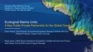
- 1. Ecological Marine Units: A New Public-Private Partnership for the Global Ocean Monterey Bay GIS User Group Stanford U. Hopkins Marine Station Pacific Grove, CA, May 25, 2017 Dawn Wright, Chief Scientist, Environmental Systems Research Institute (aka Esri) Affiliated Professor, Oregon State University Roger Sayre, USGS Senior Scientist for Ecosystems, Climate and Land Use Change Sean Breyer, Esri ArcGIS Content Program Manager
- 2. GEOSS Task EC-01-C1 (2014) / GI-14 GECO (2016) Global Ecosystem Classification and Mapping • Develop a standardized, robust, and practical global ecosystems classification and map for the planet’s terrestrial, freshwater, and marine ecosystems. • Dr. Roger Sayre, USGS, Task Lead • Esri is a partner, engaged in producing and hosting the content • Secretary Sally Jewell at the GEO 2015 Plenary in Mexico City: “The US Geological Survey and Esri will develop a new map of standardized global marine ecosystems”
- 3. Terrestrial Effort: Ecological Land Units (ELUs) Land Cover Lithology Landform Bioclimate Example: Warm Wet Plains on Metamorphic Rock with Mostly Deciduous Forest 48,872 Combinations (Facets) 3,923 Unique Land Units/Colors www.aag.org/global_ecosystems esriurl.com/elu esriurl.com/ecotapestry esriurl.com/landscape
- 4. Ecological Marine Units (EMUs) Who wants one? GEO & GEOSS (GEO BON MBON, GECO) Global Ocean Refuge System (GLORES) IUCN, WWF, CI, Mission Blue Sylvia Earle Alliance FAO and ICES OOI and IOOS/GOOS Essential Ocean Variables community (e.g., World Climate Research Program) Researchers Educators Local agencies who want the global context Natl science agencies Editors of textbooks Why? • Ecosystem Health, Resilience, Ecosystem Goods & Services; Ecosystem Services Valuation • Nature Conservation Reporting • Conservation planning • Ecosystem Classification • Ecosystem Based Management • Fisheries Management • Marine Data Management • Indicating Species Distributions • Explaining and Understanding Nature • Risk Reduction • Context: Local related to Global • System Connectivity
- 5. EMUs: • cover all the ocean • are 3D • are based on best available data • are independent of political, social and economic influence • Promote further understanding of how the environment structures biodiversity (including fisheries, threatened species, etc.) How is this different from what exists? Graphic courtesy of Mark Costello et al., U. of Auckland, New Zealand
- 6. Based on NOAA’s World Ocean Atlas 2013 v. 2 Nitrate Silicate Phosphate Temperature* Salinity Dissolved Oxygen e.g., *Locarnini, R.A., A.V. Mishonov, J.I. Antonov, T.P. Boyer, H.E. Garcia, O.K. Baranova, and others. 2013. World Ocean Atlas 2013 version 2 (WOA13 V2), Volume 1: Temperature. In: NOAA National Centers for Environmental Information S. Levitus, ed, and A. Mishonov, technical ed, NOAA Atlas NESDIS 73, doi:10.7289/V55X26VD, www.nodc.noaa.gov/OC5/woa13/ 0 m 5500 m 100 m 100 m 5 m 10 m 25 m
- 7. EMU 3D Point Mesh Framework UnitTop SurfaceArea 5500 m 100 m 100 m 5 m 10 m 25 m 0 m -5500 m Feature Attributes Depth_Level Temperature Salinity Dissolved Oxygen Nitrate Silicate Phosphate MODIS Ocean Color PointID QuarterID UnitTop (m) UnitMiddle (m) UnitBottom (m) Thickness (m) ThicknessPos (m) EMUID EMU Name GeomorphologyBase GeomorphologyFeatures SurfaceArea Volume, SpecialCases 0 m UnitBottom Unit Middle Thickness Volume World Ocean Atlas EMUPoints • K-means statistical clustering • Backwards stepwise discriminant analysis • Pseudo F-statistic 37 clusters • Canonical discriminant analysis
- 8. EMU 13 Summary Technical Name: • Bathypelagic • Very Cold • Euhaline • Hypoxic • High Nitrate • Medium Phosphate • High Silicate Common Name: • Deep • Very Cold • Normal Salinity • Low Oxygen • High Nitrate • Medium Phosphate • High Silicate
- 9. EMU 13 Summary Technical Name: • Bathypelagic • Very Cold • Euhaline • Hypoxic • High Nitrate • Medium Phosphate • High Silicate Common Name: • Deep • Very Cold • Normal Salinity • Low Oxygen • High Nitrate • Medium Phosphate • High Silicate
- 11. MobileApp App Store (iOS) or Google Play (Android)
- 12. Do Our Depth Findings Support Traditional Ocean Zonation Concepts? Figure courtesy of Paul R. Pinet, Invitation to Oceanography, 5th ed., Jones and Bartlett Publishers
- 13. Paper for peer-reviewed journal Oceanography Full Title: A Three-Dimensional Mapping of the Ocean Based on Environmental Data Short title: A 3D Mapping of the Global Oceans Author List Roger G. Sayre1, Dawn J. Wright2, Sean P. Breyer2, Kevin A. Butler2, Keith Van Graafeiland2, Mark J. Costello3, Peter T. Harris4, Kathleen L. Goodin5, John M. Guinotte6, Zeenatul Basher1, Maria T. Kavanaugh7, Patrick N. Halpin8, Mark E. Monaco9, Noel Cressie10, Peter Aniello2, Charles E. Frye2, and Drew Stephens2. 1Land Change Science Program, United States Geological Survey, Reston, Virginia, United States of America 2Esri, Redlands, California, United States of America 3Institute of Marine Science, University of Auckland, Auckland, New Zealand 4GRID-Arendal, Arendal, Norway 5NatureServe, Arlington, Virginia, United States of America 6United States Fish and Wildlife Service, Denver, Colorado, United States of America 7Woods Hole Oceanographic Institution, Woods Hole, Massachusetts, United States of America 8Nicholas School of the Environment, Duke University, Durham, North Carolina, United States of America 9National Ocean Service, National Oceanic and Atmospheric Administration, Silver Spring, Maryland, United States of America 10National Institute for Applied Statistics Research Australia, University of Wollongong, Wollongong, Australia
- 14. Ecological Marine Units (EMUs) at Depth -400m 0m -1200m -2400m -200m -800m -1800m -3800m
- 17. Dissolved Oxygen
- 18. Ocean Currents Barnier et al. Ocean Dynamics, 56: 543-567, 2006.
- 20. 3D Fence or Curtain Diagrams esriurl.com/3dfence
- 23. Next Stages ADDITIONAL DATA On the Surface OBIS More ocean color In Water Column **Seasonal TEMPORAL WOA data Particulate Organic Carbon OBIS On the Seafloor Reef/Vents features Sediment sizes **In Your Own Study Area with higher-rez data TOOLS Viewer Tools 3D Web Viewer 3D Cross Section (Fence)* Analysis Tools Compare Multiple Locations Multidimensional Range Slider 3D Kriging 3D Geo Enrichment
- 24. Next Set of Global Ecosystem Maps: ECUs and EFUs Ecological Coastal Units (ECUs) Ecological Freshwater Units (EFUs)
- 25. www.esri.com/ecological-marine-units esriurl.com/emudata geonet.esri.com/groups/ecological-marine-units www.aag.org/cs/global_marine_ecosystems Sayre et al., 2017, Oceanography, 30(1): 90-103. Nature News feature, 3 January 2017 Dawn Wright, dwright@esri.com, @deepseadawn esriurl.com/ucocean2017
Hinweis der Redaktion
- The work to produce the map and data was commissioned by the Group on Earth Observations, a mini “United Nations” of sorts consisting of almost 100 nations collaborating to build the Global Earth Observation System of Systems (GEOSS) in 9 Societal Benefit Areas (Agriculture, Biodiversity, Climate, Disasters, Ecosystems, Energy, Health, Water, and Weather). The global ecosystem mapping task, as defined here, is a key program within the GEO Biodiversity Observation Network (GEO BON) and the GEO Ecosystems Initiative (GEO ECO). One impt thing to mention is that the ELUs were released and launched as an earlier contribution to the President's Climate Data Initiative. The ELUs are now on that list of Climate Data Initiative (CDI) resources, and of course are registered on data.gov. Now the EMUs should be considered a similar contribution but for the marine environment. Since Fabien was and is apparently still engaged with the CDI, this is a major hook into White House interest. EMU is now under the new GEO Global Ecosystems initiative (GECO) arising from the GEO 2016 Transitional Workplan. The former Ecosystems Societal Benefit Area and the former Biodiversity Societal Benefit Area have been combined into a new Biodiversity and Ecosystems Sustainability SBA. The GECO is a new task, and it has four pieces to it related to 1) the European Horizon 2020 ECOPOTENTIAL project, 2) the H2020 SWOS (Satellite-based Wetlands Observation System) project, 3) global EMUs, and 4) global EFUs.
- So why do we need a global ecosystem map anyway? Such a map, and more importantly, the data, will provide scientific support for planning and management, and enable understanding of impacts to ecosystems from climate change and other disturbances. The map and data should also prove useful as an ecologically meaningful spatial accounting framework for assessments of the economic and social values of ecosystem goods and services. Should aid in REPEATABLE landscape mgmt - a platform for geo-accounting (instead of reducing so much by national boundaries, we are using real ecological units) A standard repeatable accounting framework A global view of environmental diversity Ecosystems defined by humans for humans as opposed to ecosystem HEALTH, a healthy ecosystem vs a service that the ecosystem provides - the next level to resilient ecosystems rather than ecosystem services Research goal in future? what are the indicators that if merged together in a better way would provide better services; one can still be SICK and provide services Example – indicators may be relative to the status of the fish stock but not indicators as to how the ecosystem is working. Specific needs include: Assessments of Economic and Social Value of Ecosystem Goods and Services Biodiversity Conservation Planning Analysis of Climate Change Impacts to Ecosystems (and other impacts e.g. fire, invasive species, land use, etc.) Resource Management Research Bioclimate, Landform, and Lithology = Drivers of Ecological Character (physical setting) Land Cover = Response to the Physical Setting We found 48,872 unique combinations aggregated to 3923 ELUs. In 2015 106,959 unique combos thanks to the updated land forms and land cover, 2010 epoch, Global Land Cover, v. 1.4 Bioclimate, Landform, and Lithology = Drivers of Ecological Character (physical setting) Land Cover = Response to the Physical Setting Bioclimates - Global Environmental Stratification (GEnS), U. of Edinburgh - 50 year avg of temp/precip from met stations throughout world 30 arc sec raster, down-sampled to 250-m raster Landforms – USGS – 250-m raster, derived from GMTED2010 Surficial Lithology - Global Lithological Map (GLiM), Hamburg University, Vector Polygons converted to 250-m raster Land Cover - GlobCover, 2009, European Space Agency - MARIS satellite, 300 m rez resampled to 250 m Version 2 recently released in 2015 with updated land cover, 2010 epoch, Global Land Cover, v. 1.4 Only layer that we had an option: GlobCover 2009, GlobeLand30 or MDA’s NaturalVue GlobCover 2009 offered a richer, more flexible classification, which is compatible with USGS NLCD NaturalVue was too old. Both had significant quality issues relative to broad audience acceptance Today, there are more options. Globeland30 continues to be improved. MDA has produced BaseVue How did we make the map? Again, we define ecosystems as distinct physical environments and their associated vegetation, so we map ecosystems by first mapping, and then combining in a GIS, global bioclimates, global landforms, global geology, and global land cover. Characterize the principle ecological land components of the terrestrial surface of the earth in a micro-scale, bottom-up, hierarchical classification process. Subdivide the land surface of the earth into macro-scale physiographic (geomorphological) areas in a top-down, hierarchical regionalization process. Combine the physiographic regionalization process with the ecological classification process to develop a hierarchical, ecophysiographic segmentation of the planet. Weightings of 4 layers: 3, 3, 2, 1
- Instead of reflecting JUST researchers perceptions and local experiences, our EMUs provide quantifiable definitions for these such as epipelagic, mesopelagic, bathypelagic, etc.
- Where do we get the best “physical setting” for the ocean, which will in turn drives its ecological character? WOA is probably the best available set of “objectively analyzed climatologies” for the major physical parameters of the world’s oceans (interpolated mean fields at standard depth levels). From NOAA NCEI (formerly NODC), http://www.nodc.noaa.gov/OC5/woa13/ SPATIALLY WOA 2013 at finest rez of ¼ degree (27 km at equator) for all variables save for nutrients at 1 km (subsampled nutrients so there is a slight source of error there) ¼ deg horiz and vertical, 102 depth zones ranging in thickness from 5 m at surface to 500 m in deep ocean TEMPORALLY WOA 2013 has 5 or 6 decadal averages - 1 point in our mesh is the avg of a 57-year period, so it’s an average of an average of the prominent mean over 50 years - trying to conceptualize regions as long-term historical average, possibly stable WOA has seasonal averages – we are not dealing with those – we assume that these are already part of the annual/decadal but this is the next logical step, to do clustering on monthly avgs as part of a later study; once we understand the decadal we can apply to quarterly/seasonal intervals
- NOAA administrator Kathryn Sullivan likens this to a “christmas tree” that we ALL can hang ornaments on now. In GIS-speak this means additional Feature Attributes Step 1 - Build 3-D framework (point mesh), where we extracted the World Ocean Atlas data into a global point mesh framework created from 52,487,233 points, each with at least 6 WOA attributes Step 2 - Attribute mesh points with 6 WOA physical/chemical parameters, in addition to the x, y, and z coordinates (more attributes possible) Step 3 – Used k-means statistical clustering algorithm to identify physically distinct, relatively homogenous, volumetric regions in the water column (EMUs). Backwards stepwise discriminant analysis to determine if all of six variable contributed significantly to the clustering – all six were significant. pseudo F-statistic gave us the optimum # of clusters at 37. Then used canonical discriminant analysis to verify that all 37 clusters were significantly different from one another and they were. Compare/combine surface-occurring EMUs with other sea surface partitioning efforts using ocean color, etc. (e.g., Longhurst, Oliver and Andrew, MBON, Seascapes, etc.) Compare/combine bottom-occurring EMUs with seafloor physiographic regions and features, etc. (e.g., Harris et al.) Assess relationship between physically distinct regions and biotic distributions (e.g., OBIS Biogeographic Realms, etc.), and maybe combine to incorporate biotic dimension into the EMUs [In the weeds: A globally comprehensive subset (25,000 points) of all points was used for the determination of the optimum cluster number using the pseudo F-statistics, yielding an optimum of 37 clusters. For the approach, the approximately 52 million global points were then clustered in a series of sequential iterations where the number of clusters requested ranged from 5 to 500, increasing the cluster number by ten for each successive iteration.]
- Example summary of an EMU. There is one for each of the 37
- You can download this from your seat right now, but especially for you young people, I hope you’ll stay pay attention during the remainder of my talk!
- Most oceanography and marine biology textbooks include diagrams dividing the oceans into depth zones. Although depth boundaries for these regions are largely arbitrary and can vary from text to text, they are meant to describe the ecological variation that is correlated with depth. It is possible that sea temperature and physiographic features (e.g. abyssal plain) create distinct zones differing in environmental conditions with depth, and these conditions may be reflected in different ecological communities. However, this has never been objectively tested using data at a global scale most existing marine maps and zonation systems are derived from supervised classification and thus biased by the experiences and perspective of their authors and the availability of observations in particular regions
- This article now appears in Oceanography, 30(1): 90-103, 2017.
- HORIZONTALLY on the LEFT VERTICALLY on the RIGHT ON THE LEFT: 37 mutually exclusive EMU clusters (shown with ELUs) representing the maximum global horizontal dimensions of the clusters AT SELECTED DEPTHS AND in different colors. While a total of 37 EMUs were statistically determined, a number of them are small, localized, and shallow, and are not discernible in these depth-layer maps. Black indicates regions shallower than the depth at that layer. Major hydrographic features like Northern and Southern Hemisphere gyre systems and coastal upwelling-based westward flow of water from western continental margins are evident, particularly at shallower depths (upper left and right panels). Colors reflect mean EMU temperatures, with pink colors representing warmer EMUs and blue colors representing colder EMUs. ON THE RIGHT: Vertical profile area graph with depth on Y-axis and cell count for each Cluster/area it covers on X-axis. This graph shows the cluster variety at the top of the water column and through the water column we can see how each Cluster either slowly disappears with depth or in some cases deep water clusters become more dominant. It also help illustrate how in some cases the cluster is spread across the CMECS depth terms and we may need a better data-driven depth name for the clusters. Interesting too that there are apparent depths where groups of clusters end -100 to -200m and -500 to -700m and -1400 to -1600m. Our diagram illustrates that there is no simple clear-cut HORIZONTAL boundary for water attributes – an overlay of depth distribution on it will also be informative The two-dimensional global area (km2) at any depth is shown for the 22 EMUs that comprise 99% of the ocean volume. The horizontal boundary lines separating the depth zone classes are as described in the Coastal and Marine Ecosystem Classification Standard (CMECS), the Federal Geographic Data Committee (FGDC) standard for the United States (FGDC, 2012). The EMU number labels are placed at the median unit-middle depth for each EMU. Although the EMUs are not uniformly distributed into the CMECS depth zones, strong vertical separation is evident, with many small EMUs in the upper water column and fewer larger EMUs in the middle and lower water columns. Pink colors indicate warmer EMUs, and blue colors indicate colder EMUs.
- How do we best visualize something that is really continuous and in 3D? One way is to conceptualize the data as columnar stacks of cells whose centroids define the point mesh In live presentation there was a VIDEO flythrough that took us up the US west coast, stopping at Monterey Canyon. As we zoom in, cylinders will pop up, representing data points from NOAA’s World Ocean Atlas, 52 million observations over a span of 50 years about the primary physical and chemical characteristics of the oceans at 105 depth levels: in other words, the key variables that enable life throughout the ocean such as salinity, temperature, dissolved oxygen, phosphate, nitrate, silicate. This is actually a continuous grid of data at the surface and continuous volumes at depth but we are representing the units as columns so that you can see sideways better into the layers at depth. One major point is that nutrient and oxygen distributions in particular not only shape but ARE SHAPED by biological processes (physicochemical). This information will be hugely significant biologically, to be able to see that over a global expanse, where it thins out, where it mixes with other water masses. This is a global framework. Will soon start time slicing into monthly averages, OBIS has not been added to this yet, but that is in progress. It will be exciting to be able to continually populate and improve this with data from any cruise or expedition as we go forward in time. NOAA administrator Kathryn Sullivan likens this to a christmas tree that we ALL can hang ornaments on now, and over time really come to a richer understanding of our ocean, while also helping us to understand what’s the next science data or target we should go after to make this more useful, especially for MPA designation or evaluation and CMSP.
- From the main EMU web site.
- Dissolved oxygen column, south of Tasmania
- We integrated global ocean currents directly into the Ecological Marine Units point mesh. The data came to us courtesy of Bernard Barnier <bernard.barnier@univ-grenoble-alpes.fr> and his colleagues in the DRAKKAR consortium, a scientific and technical coordination between French research teams (LGGE-Grenoble, LPO-Brest, LOCEAN-Paris), MERCATOR-ocean, NOC Southampton, IFM-Geomar Kiel, and other teams in Europe and Canada. They have designed, assessed, and distributed high-resolution global ocean/sea-ice numerical simulations based on the NEMO platform as performed over long periods (five decades or more). The ocean currents were produced by their eddy-permitting ORCA12 model, thus far the highest resolution global realistic model of the DRAKKAR hierarchy (Barnier et al., 2006, Drakkar Group, 2014). The grid size of ORCA12 is 9.25 km at the Equator, 4 km on average in the Arctic, and up to 1.8 km in the Ross and Weddell seas. The model uses 46 vertical levels with a vertical grid spacing finer near the surface (6 m) and increasing with depth to 250 m at the bottom. The model simulation which produced the present ocean currents is part of a series of high resolution model hindcasts aimed at representing the ocean circulation from the 1960s to present (DRAKKAR Group, 2014). It was driven by the DFS4.4 atmospheric forcing that combines satellite observations with ERA40 and ERA interim analytics into a single 6-hourly forcing set for the period 1958-2012 (Dussin et al., 2016), using the methodology developed by Brodeau et al. (2010). The currents within the EMUs are the climatological mean for the period 2000-2012. The original 1/12° resolution currents were interpolated onto the 1/4° standard resolution grid that is the basis for our EMUs. References: Barnier, B., G. Madec, T. Penduff, J.M. Molines, A.M. Treguier, J. Le Sommer, A. Beckmann, A. Biastoch, C. Böning, J. Dengg, C. Derval, E. Durand, S. Gulev, E. Remy, C. Talandier, S. Theetten, M. Maltrud, J. McClean, B. De Cuevas 2006: Impact of partial steps and momentum advection schemes in a global ocean circulation model at eddy permitting resolution. Ocean Dynamics, 56, 543-567, DOI: 10.1007/s10236-006-0082-1. DRAKKAR Group (, B. Barnier, A.T. Blaker, A. Biastoch, C.W. Böning, A. Coward, J. Deshayes, A. Duchez, J. Hirschi, J. Le Sommer, G. Madec, G. Maze, J. M. Molines, A. New, T. Penduff, M. Scheinert, C. Talandier, A.M. Treguier), 2014: DRAKKAR: Developing high resolution ocean components for European Earth system models. CLIVAR Exchanges Newsletter, No.64 (Vol 19, No.1). Madec,G., 2008: NEMO ocean engine, Note du Pole de modelisation, Institut Pierre-Simon Laplace (IPSL), France, No 27 ISSN,1288–1619. Brodeau, L., B. Barnier, A.M. Treguier, T. Penduff, S. Gulev, 2010: An ERA40-based atmospheric forcing for global ocean circulation models. Ocean Modelling, 31, 88-104, doi: 10.1016/j. ocemod.2009.10.005. Dussin, R., B.Barnier and L. Brodeau, 2016. The making of Drakkar forcing set DFS5.DRAKKAR/MyOcean Report 01-04-16, LGGE, Grenoble, France. Akima, H., 1970: A New Method of Interpolation and Smooth Curve Fitting Based on Local Procedures. J. ACM, 17 (4), 589-602, doi: 10.1145/321607.321609.
- From the main EMU web site.
- We can use 3D analysis to create vertical fences as a way of interpolating the water column. In this example points were measurements of oil in seawater after an oil spill with concentrations of the pollutant from the surface down to a certain depth interpolated into a ”fence” or curtain.” This tool is now free, open and available for download at esriurl.com/3dfence. The Parallel Fences option of the tool can generate sets of parallel fences in directions that are related to either longitudes, latitudes, or depths. The Interactive Fences tool can generate fences based on lines digitized on the map GIS deep dive: a free ArcGIS ToolBox called “3D Fences” cuts slices through 3D point data and applies empirical bayesian kriging analysis to the slices (including error surfaces). Internally the tool uses Empirical Bayesian Kriging (EBK) to interpolate values between samples and then converts the EBK output to points for display. The tools provide an option to output either EBK Prediction or EBK Prediction Standard Error as well as options to control minimum fence dimensions, sample points and interpolation resolution. Motivated and curious python savvy users can easily change the interpolation method employed by the tools if input data warrant use of a different method or a Geostatistical Analyst license is unavailable
- Fence diagrams from EMU data across the Puerto Rico Trench (salinity). This is from a demo and not yet released to the public, but coming soon.
- To stay apprised of progress and to interact with the project team further, I strongly encourage you to join the Ecological Marine Units discussion group, a discussion group of the GeoNet community. If not already familiar with the GeoNet community, there are helpful guidelines at https://geonet.esri.com/docs/DOC-9165-what-is-geonet .
- Regarding additional data to be added to EMUs, POC may be useful more as a validation of the clustering rather than as input for wholesale reclustering (POC data are scattered, hard to obtain from Lutz or to compile from NASA, hard to recalculate for entire global water column)
- We plan on holding a kickoff meeting for the ECU component on October 31st as a sidebar meeting within the next Esri Ocean GIS Forum in Redlands – so bookmark http://www.esri.com/events/ocean .
- See the new EMU story map at http://esriurl.com/emustory