Test file for mfpic4ode package: Phase portraits and numerical methods
1. Test file for mfpic4ode package
Robert Maˇ´
rık
April 15, 2009
See the source file demo.tex for comments in the TEX code.
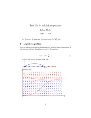
1 Logistic equation
Here we draw a simple picture which describes stability of stationary points of
teh equation and then draw phase portrait of the equation.
x
x =r· 1− x (1)
K
Stability and sign of the right–hand side.
f (x)
x
K
Phase portrait
x
K
t
1
2. 2 Logistic equation with harvesting
Similar to the previous picture, but both pictures are drawn together to see the
relations between them.
x
x =r· 1− x−p (2)
K
x x
K K
f (x)
t
3 Three numerical methods for ODEs
Here we draw solution of ODE using all three available numerical methods. We
use big step to see the difference between Euler, Runge–Kutta and fourth order
Runge–Kutta method.
xn+1 = xn + h
y = x + y3
yn+1 = yn + kh
y(0) = 1
h = 0.2
2
3. 2.4 Exact solution
2.2
RK4
RK
2
1.8
1.6 Euler
1.4
1.2 k1 for second step
k2
1 k
1
0 0.2 0.4
0.8
4 Autonomous systems
We draw the phase portrait of autonomous system, nulclines, invariant set be-
tween nulclines, trajectories. We draw arrows in regular grid and add few more
arrows on nulclines and outside the regular grid.
3
4. y Competing species
a
c
α
β
α a
x
γ b
Pedator prey system with HollingII response function
y
x
4