1. SECTION 1. AERODYNAMICS OF LIFTING SURFACES
THEME 4. THE AERODYNAMIC CHARACTERISTICS OF
WINGS IN A FLOW OF INCOMPRESSIBLE FLUID
The main aerodynamic characteristics of an aircraft moving with Mach numbers
( M ∞ ≤ 0 .4 ) are considered in this lecture.
4.1. Wing lift coefficient
4.1.1. High-aspect-ratio wings
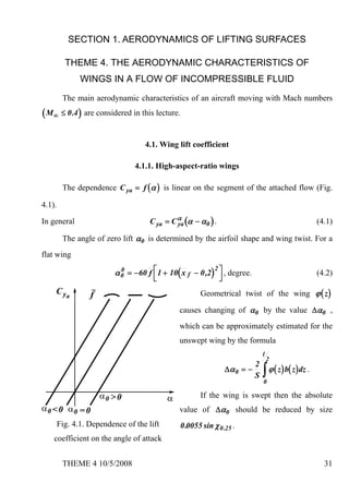
The dependence C ya = f ( α ) is linear on the segment of the attached flow (Fig.
4.1).
In general C ya = C α (α − α0 ) .
ya (4.1)
The angle of zero lift α0 is determined by the airfoil shape and wing twist. For a
flat wing
α 0 = −60 f ⎡ 1 + 10( x f − 0 ,2) ⎤ , degree.
0 2
⎢ ⎥ (4.2)
⎣ ⎦
Geometrical twist of the wing ϕ ( z )
causes changing of α0 by the value Δα0 ,
which can be approximately estimated for the
unswept wing by the formula
l
2
2
Δα 0 = −
S ∫ ϕ ( z) b( z) dz .
0
If the wing is swept then the absolute
value of Δα0 should be reduced by size
Fig. 4.1. Dependence of the lift 0 .0055 sin χ 0 .25 .
coefficient on the angle of attack
THEME 4 10/5/2008 31

2. The derivative C α depends on aspect ratio λ and the sweep angle χ , influence of
ya
taper η on derivative size is weak. The derivative C α does not depend on wing twist.
ya
It is possible to offer the following approximate formula for calculation of value of
Cα :
ya
πλ λ
Cα =
ya , m= (4.3)
α
1+τ + (1 + τ ) 2
+ ( π m)
2 C ya∞ cos χ 0 .5
Here the parameter τ takes into account the wing plan form and depends on η ,
λ , χ 0 .5 . It is possible to assume in the first approximation τ ≈ 0 (in general
τ ≈ 0 ...0 ,24 ),
⎡ ⎤
2 1 ⎥.
τ = 0 ,17 m ⎢η + (4.4)
⎢
⎣ (5η + 1) ⎦
3⎥
Parameter C α
ya∞ is a derivative for the airfoil (wing with λ → ∞ ) and is
calculated by the formula
(
C α = 2π − 1,69 4 c = 2π 1 − 0 ,27 4 c .
ya∞ ) (4.5)
It follows from the formula, that at λ → ∞ C α = C α ∞ cos χ 0 .5 and if in
ya ya
addition χ 0 .5 = 0 , then C α = C α ∞ .
ya ya
It is also possible to use the following formula for calculation C α :
ya
α Cα ∞ λ
ya
C ya = . (4.6)
1 α
pλ + C ya∞
π
Here p is the ratio of half-perimeter of the wing outline in the plan to span (Fig.
4.2). The significance of the last formula is in its universality and capability to apply to
any plan forms and aspect ratios (it is especially useful for wings with curvilinear edges
or edges with fracture).
THEME 4 10/5/2008 32

3. It is possible to define parameter p for
a wing represented in fig. 4.2, by the formula
l1 + l2 + l3 + l4
p= , or in case of tapered
l
wing - by the formula
⎛ 1 1 ⎞ 2
p = 0 .5 ⎜ + ⎟+ .
⎝ cos χ п .к . cos χ з .к . ⎠ λ (η + 1)
Fig. 4.2.
Let's analyze the influence of wing
geometrical parameters on value C α .
ya
1. With increasing of wing aspect ratio
λ the derivative of a lift coefficient on the
angle of attack C α grows (at conditions of
ya
χ = 0 and λ → ∞ the value of a derivative
tends to the airfoil characteristic C α = C α ∞
ya ya
(Fig. 4.3).
Fig. 4.3.
2. With increasing of sweep angle at
half-line chord ( 0 .5 chord line χ 0 .5 ) the
derivative value C α decreases (Fig. 4.4). (It
ya
occurs due to effect of slipping, at condition
of λ → ∞ , the sweep angles on the leading
and trailing edges are identical
χ l .e .≈ χ t .e .= χ , C α = C α ∞ cos χ ).
ya ya
3. The sweep influence on derivative
C α value decreases with decreasing of
ya
Fig. 4.4.
aspect ratio λ (Fig. 4.5) (sweep practically
THEME 4 10/5/2008 33

4. does not influence on value of lift coefficient
derivative on the angle of attack C α at small
ya
values of aspect ratio λ ).
4. The wing taper η influences a little
onto the value of a derivative C α (refer to
ya
formula (4.4), parameter τ ).
Fig. 4.5.
4.1.2. Wings of small aspect ratio
It is necessary to take into account the non-linear effects which occur at flow
about wings of small aspect ratio in dependence of a lift coefficient on the angle of
attack C ya = f ( α ) (Fig. 4.6)
C ya = C ya line + ΔC ya
where C ya line = C α (α − α 0 ) .
ya
It is also possible to define values of
α 0 and C α by the formulae for large aspect
ya
ratio wings at λ ≥ 2 The value of derivative
can be determined by the formula
Fig. 4.6.
Cα = π λ
ya for a wing of extremely small
2
aspect ratio λ < 1 , and the angle of zero lift for the wing with unswept trailing edge is
( )
equal to an angle of the trailing edge deflection α 0 = f ′ x t .e . , z , where y = f ( x , z ) -
∂ f
equation of a surface of a wing, f ′ = , x t .e . is trailing edge coordinate.
∂x
THEME 4 10/5/2008 34

5. The non-linear additive can be calculated by the formula which is fair at any
Mach numbers (the linear theory of subsonic flow refers only to a linear part of the
dependence).
4C α
1 − M ∞ cos 2 χ l .e . ⋅ (α − α 0 )
ya 2 2
ΔC ya = (4.7)
πλ
At a supersonic leading edge ( M ∞ cos χ l .e . > 1 ) the non-linear additive
disappears and ΔC ya = 0 .
With decreasing of λ the derivative C α decreases, and the non-linear additive
ya
ΔC ya grows (Fig. 4.7, 4.8).
Fig. 4.7. Character of changing of the non- Fig. 4.8. Character of changing of the non-
linear additive ΔC ya linear additive ΔC ya
4.2. Maximum lift coefficient.
The maximum lift coefficient is connected with the appearance and development
of flow stalling from the upper wing surface near the trailing edge and depends on many
factors, first of all, on the characteristics of the airfoil ( c , f , x f , nose section shape),
wing plan form ( χ , η ), Reynolds number Re . The λ value does not practically
THEME 4 10/5/2008 35

6. influence onto C ya max for wings of large aspect ratio (Fig. 4.9), at that with χ
decreasing α st increases.
The influence of λ has an effect as follows for wings of small aspect ratio:
C ya max grows with λ growing from 0 up to λ ~ 1 ; and then decreases - with
increasing of λ . Small values of C ya max ( C ya max ≈ 1,0 ...1,1 ) and large values of α st
( α st ≈ 25 o ...40 o ) (fig. 4.10) are characteristic for wings with λ < 3 . A flow stalling
delays in the latter case caused by influence of vortex structures formed on the upper
wing surface.
Fig. 4.9. Dependence C ya = ( α ) for Fig. 4.10. Dependence C ya = ( α ) for
wings of large aspect ratio λ ≥ 4 . wings of small aspect ratio λ < 3
The properties behaviour of curve C ya (α ) in area α st depends on the nose
section shape. The presence of C ya max low values is characteristic for a wing with the
pointed airfoil nose section which do not depend on Reynolds numbers (Fig. 4.11). The
increasing of C ya max (up to certain values) is characteristic for a wing with the rounded
airfoil nose section at increase of Reynolds numbers (Fig. 4.12).
Approximately, value C ya max of large aspect ratio wing ( λ ≥ 4 ) can be
determined by the formula
THEME 4 10/5/2008 36

7. ⎛ 0 .49η + 0 .91 2 ⎞ ⎡ η+2 ⎤
C ya max = C ya max ∞ ⎜ 1 − sin χ 0 .25 ⎟ ≈ C ya max ∞ ⎢1 − sin2 χ 0 .25 ⎥ ,
⎝ η+1 ⎠ ⎢
⎣ 2(η + 1) ⎥
⎦
where C ya max ∞ is the maximum value of an airfoil lift coefficient;
for symmetrical airfoil C ya max ∞ ≈ 35 c exp − 8 c at Reynolds numbers Re ≤ 10 6 and
( )
C ya max ∞ ≈ 39 .3 c exp − 8 c th Re⋅ 10 − 6 at Re ≥ 10 6 .
Fig. 4.11. Dependence C ya = ( α ) for Fig. 4.12. Dependence C ya = ( α ) for
wings with a sharp leading edge wings with a classical airfoil
Number Re is the kinematic factor of similarity describing the ratio of inertial
and viscous forces:
VL
Re = , (4.8)
ϑ
Where V is the characteristic speed; L is the characteristic length; ϑ is the kinematic
factor of viscosity.
THEME 4 10/5/2008 37

8. 4.3. Induced drag.
It is a result of the appearance of a vortex sheet behind a wing, which keeping
demands energy equivalent to work of induced drag force. The computational formulae
for definition of C xi are described below.
4.3.1. Wings of large aspect ratio
The induced drag coefficient of a large aspect ratio wing is determined
C xi = C xi ϕ = 0 + ΔC xiϕ , (4.9)
Where C xi ϕ =0 is the induced drag of a flat wing; ΔC xiϕ is the additive to induced drag
caused by geometrical twist.
We have
1+δ 2 2 1+δ
C xi ϕ = 0 = C ya = AC ya , A = (4.10)
π ⋅λ π ⋅λ
Dependence of induced drag at small angles of attack is approximated by
parabola (Fig. 4.13). The induced drag decreases at increasing of wing aspect ratio λ .
The coefficient δ is determined by the wing plan form and shows to what extent
the distribution of aerodynamic loading differs from the elliptical law, for which δ = 0 .
Generally δ ≈ 0 ...0 .10 . The expression for C xi ϕ =0 is represented as
1 2 1
C xi ϕ = 0 = C ya lately, where e is Osvald number, e = .
πλe 1+δ
Value of ΔC xi ϕ in contrast to C xi ϕ =0 can not be equal to zero in general at
C ya = 0 (because for non-flat wing various wing cross-sections may have lift
coefficients not equal to zero C ya ≠ 0 at total C ya = 0 ).
General expression for ΔC xiϕ looks like this: ΔC xiϕ = BC ya + C , where,
2
B = к 1ϕ w , С = к0ϕ w , ϕ w is the twist angle of tip cross-section; the values of
coefficients к0 and к 1 are also undertaken from the diagrams depending on wing plan
geometry ( λ , χ , η ), and twist law.
THEME 4 10/5/2008 38

9. Fig. 4.14. shows the comparison between induced drag of a flat wing and wing
having twist.
Fig. 4.13. Induced drag of a flat wing Fig. 4.14. Induced drag of a flat wing and
wing with twist
4.3.2. Wings of small aspect ratio
For a geometrically flat wing it is possible to assume:
C xi ϕ = 0 = C ya ⋅ α . (4.11)
This expression can be received if it is assumed that the sucking force is not
realized on the wing leading edge. The formula can be transformed to the following
form if the non-linear additive is neglected ( ΔC ya = 0 ) we have:
C xiϕ = 0 = AC ya , A = 1 C α
2
ya (4.12)
In such form the formula is used in practice (it coincides with the formula for a
flat wing of large aspect ratio)
πλ 2
( For a wing of small aspect ratio λ < 1 , C α =
ya and A = ; comparing
2 πλ
1+δ
with a wing of large aspect ratio A = we shall notice that δ = 1 ).
π ⋅λ
THEME 4 10/5/2008 39

10. 4.4. Wing polar
Polar of the first type is called the dependence between coefficients of
aerodynamic lift and drag force C ya = f (C xa ) . As well as the induced drag coefficient
the polar depends on twist presence on a wing. Therefore we shall separately consider
polar for a flat wing and polar for a wing having twist, and we shall conduct the
qualitative analysis.
4.4.1. Flat wing.
Summing induced drag C xi with profile drag C xp , we shall receive expression
for polar:
2
C xa = C xp + C xi = C xp + AC ya . (4.13)
It can be assumed that the profile drag
C xp does not depend on a lift coefficient C ya
( )
C xp ≠ f C ya . In this case we shall write
2
down C xa = C x 0 + AC ya , where C x0 is the
wing drag coefficient at C ya = 0 (in this case
Fig. 4.15. Dependence of profile drag it coincides with C xp ). It is necessary to note
on lifting force
that in general the profile drag C xp changes
2
by C ya especially at large values of α or C ya , it is approximately proportional to C ya
(Fig. 4.15); in some cases this change is taken into account in parameter A :
2 2 ~ 2 2
C xa = C x0 + aC ya + AC ya = C x0 + AC ya = C x0 + AC ya , (4.14)
~ 1+δ 1+δ 1
Where A = A + a ; for high-aspect-ratio wings A = and a + = ,
πλ πλ π λ ef
THEME 4 10/5/2008 40

11. 0 .95 λ
λ ef = ).
1 + 0 .16 λ tgχ 0 .5
The last polar writing (4.14) is the most
general form, which is fair for any
aerodynamic shapes if not to decipher
parameters C x0 and A . Parameter A has the
name of a polar pull-off coefficient.
∂ C xa
Obviously, that in general A = . Wing
2
∂ C ya
profile drag C xp does not depend on λ and
polar for wings of various aspect ratio λ are
look like as it is shown on fig. 4.16. As it was
Fig. 4.16. Flat wing polar
spoken earlier, the induced drag decreases
with increasing of aspect ratio λ , and consequently the drag C xa for a wing of infinite
aspect ratio λ → ∞ (airfoil) will be equal to profile drag C xp or C x0 .
4.4.2. Non-planar wings (wings with geometrical twist).
A The general form of polar equation for a non-planar wing
2
C xa = C + BC ya + AC ya , where profile drag C xp and part of induced drag caused by
2
wing geometrical twist enter parameter C , i.e. C = C xp + к0 ϕ w . Parameter B is also
determined by wing twist B = к 1ϕ w . The polar pull-off coefficient does not depend on
wing twist.
Polar equation for a wing with geometrical twist is a square parabola with
displaced peak (Fig. 4.17). It is possible to write down
2
B2
C xa =C−
4A
⎛
+ A⎜ C ya +
⎝
B⎞
(
⎟ = C xa min + A C ya − C yam
2 A⎠
)2 , (4.15)
THEME 4 10/5/2008 41

12. B2 B
Where C xa min = C − ; C yam = − .
4A 2A
From comparison of polar for flat and non-planar wings (the Fig. 4.18) it is
possible to reveal the advantages of using of a non-planar wing:
1. At C ya > C 0 twisted wing drag is less than ΔC xa = C xa tw − C xa
ya flat <0
2. The maximum lift-to-drag ratio of a non-planar wing is higher
K max tw > K max flat . (The wing is staying non-planar at mechanization deflection but
K max tw < K max flat ).
Fig. 4.17. Polar for a wing having twist Fig. 4.18. Polar for a flat and non-planar
(for a non-planar wing) wings
In addition, due to geometrical twist it is possible to provide wing balancing
without increase of induced drag (non-planar wing is self-balanced). It is easy to see,
that the advantages of a non-planar wing are shown at condition of B < 0 . In this case
polar peak displaces upwards.
4.5. Lift-to-drag ratio.
The ratio of aerodynamic lift to the drag force obtained by dividing the lift by the
drag is called lift-to-drag ratio K :
THEME 4 10/5/2008 42

13. C ya
K= , (4.16)
C xa
The lift-to-drag ratio is one of the basic characteristics determining efficiency of
an airplane.
C ya
For a flat wing K = . (4.17)
2
C x0 + AC ya
Fig. 4.19 shows the dependence of
K = f ( C ya ) . The lift coefficient and angle of
attack at which maximum lift-to-drag ratio
K max is achieved is called as optimal and
designated as C ya opt and α opt .
Let's define maximum lift-to-drag ratio.
For this purpose we shall differentiate K by
C ya and from the condition
2
∂K C x 0 + AC ya − 2 AC ya
= =0
Fig. 4.19. Dependence K = f ( C ya ) ∂ C ya
( 2 2
C x0 + AC ya )
we shall define values C ya at which the lift-to-drag ratio has extremes:
C x0
C ya opt = .
A
We shall receive the formula for calculation of maximum quality having
C x0
substituted C ya opt = in expression (4.17). We get
A
C x0
A 1
K max = ; K max = .
2 2 AC x 0
⎛ C x0 ⎞
C x0 + A⎜ ⎟
⎝ A ⎠
THEME 4 10/5/2008 43

14. The value of K max is increased with increasing of λ , decreasing of C x0 and δ
(δ = 0 for elliptical distribution of chordwise). We shall notice, that
1
K max ⋅ C ya opt = and does not depend on C x0 .
2A
C ya 1
For a non-planar wing - K = and K max = .
2 2 AC x 0 + B
C x0 + BC ya + AC ya
It is easy to find values of K max , C ya opt , α opt graphically. It follows from fig.
4.20 that it is necessary to conduct a beam tangent to polar from origin of coordinates to
search K max . The values of C ya and α in tangency point will correspond to C ya opt
and α opt .
Fig. 4.20. Dependencies C ya = f ( α ) , K = f ( α ) , C ya = f (C xa ) and connection
between them.
4.6. Distribution of aerodynamic loading along wing span.
Summarizing pressure distribution chordwise, we receive C ya се ÷ = f ( z ) .
Analysing the influence of wing geometrical parameters in planform on distribution of
THEME 4 10/5/2008 44

15. C ya cr .s .
aerodynamic loading spanwise it is convenient to use relative value C ya сr .s . = .
C ya
The function C ya cr .s . = f ( z) depends on λ , χ , η and geometrical twist (refer to
Fig. 3.5). Let's consider a flat wing. The influence of λ , χ , η is shown on the
following diagrams (Figs. 4.21, 4.22, 4.23).
Loading is distributed spanwise more regular with increasing of aspect ratio λ
.At λ = ∞ and for an elliptical wing C ya се ÷ = 1,0 . Refer to fig. 4.21.
The increasing of sweep angle χ causes growth of loading in a tip part and
reduction in root cross-section for a swept-back wing ( χ > 0 ). Refer to fig. 4.22.
The influence of wing taper η is similar to sweep χ effect : there is loading
growth in wing tip cross-sections with taper η increasing. Refer to fig. 4.23.
Distribution of lift along wing span:
Fig. 4.21. Depending on Fig. 4.22. Depending on Fig. 4.23. Depending on
aspect ratio at condition of sweep at condition of taper at condition of
χ = 0 , η = const = 1 λ = const , η = const λ = const , χ = 0
It is possible to write down approximately for a one-profile flat high-aspect-ratio
wing:
THEME 4 10/5/2008 45

16. ⎡ Cα ∞ ⎤ 1− z
2
2 ⎛
( 3 + τ )⎥ ⎜ 1 − cos χ 1 ⎞ ( 1 − z ) ; 0 ≤ z ≤ 1 ,
ya
C ya cr .s . = ⎢ 1 + − ⎟
⎢ πλ ⎥ 3μ + 1 − z 2 b( z ) ⎝ 4⎠
⎣ ⎦
Cα ∞
b( z ) , C α ∞ = 2π − 1,69 4 c , the values of parameter τ = f (λ , χ , η )
ya
Where μ = ya
4λ
are taken from the reference book or calculated.
Chords are distributed spanwise for a tapered wing with straight-line edges as
η − (η − 1) z
follows: b( z ) = 2 .
η+1
⎡ ⎤
⎢η 2 + 1 ⎥, m = λ 1
Approximately τ = 0 .17 m ,η= .
⎢
(5η + 1) 3 ⎥ C α ∞ cos χ 0 .5
ya
η
⎣ ⎦
4.7. Flow stalling.
Different values of C ya cr .s . along wing span are the reason of flow stalling in one
of cross-sections in which the local value C ya max cr .s . is reached. For example, the flow
stalling on a flat rectangular wing occurs at increasing of angles of attack in central
cross-section. It is evidently shown in fig. 4.24., that the true angle of attack in central
cross-section of a rectangular wing is more than at the tip α real 1 > α real 2 , therefore
flow stalling will begin in that place, where the true angle of attack comes nearer to
critical.
Fig. 4.24.
THEME 4 10/5/2008 46

17. In general the position of flow stalling spanwise on a tapered unswept wing can
be determined by the formula z stall ≈ 1 − η , for swept tapered wing the position of
stalling spanwise is determined by the following dependence
1−η + a ( 1 + a ) 2 − (1 − η ) 2
z stall ≈ , a = π η (1 − cos χ 0 .25 ) .
1 + a2
For improvement of wing aerodynamics at high angles of attack it is necessary to
create a condition of simultaneous flow stalling spanwise, i.e. uniform distribution of
loading spanwise It can be achieved by geometrical twist application. It is necessary to
apply wash-in to rectangular wing for the purpose of increasing loading in tip cross-
sections, wash-out is used for unswept wing, in this case tip cross-sections are unload.
(It has be noticed, that for a wing with the elliptical law of chords distribution spanwise
without geometrical twist all cross-sections have an identical C ya cr .s . , because
Vi = const and real angles of attack α real = const are identical for such wing
spanwise).
THEME 4 10/5/2008 47