thesis version before the defense

1. Numerical methods for stochastic systems subject
to generalized L´evy noise
by
Mengdi Zheng
Sc.B. in Physics, Zhejiang University; Hangzhou, Zhejiang, China, 2008
Sc.M. in Physics, Brown University; Providence, RI, USA, 2010
Sc.M. in Applied Math, Brown University; Providence, RI, USA, 2011
A dissertation submitted in partial fulfillment of the
requirements for the degree of Doctor of Philosophy
in The Division of Applied Mathematics at Brown University
PROVIDENCE, RHODE ISLAND
April 2015

2. c Copyright 2015 by Mengdi Zheng

3. This dissertation by Mengdi Zheng is accepted in its present form
by The Division of Applied Mathematics as satisfying the
dissertation requirement for the degree of Doctor of Philosophy.
Date
George Em Karniadakis, Ph.D., Advisor
Recommended to the Graduate Council
Date
Hui Wang, Ph.D., Reader
Date
Xiaoliang Wan, Ph.D., Reader
Approved by the Graduate Council
Date
Peter Weber, Dean of the Graduate School
iii

4. Vitae
Born on September 04, 1986 in Hangzhou, Zhejiang, China.
Education
• Sc.M. in Applied Math, Brown University; Providence, RI, USA, 2011
• Sc.M. in Physics, Brown University; Providence, RI, USA, 2010
• Sc.B. in Physics, Zhejiang University; Hangzhou, Zhejiang, China, 2008
Publications
• M. Zheng, G.E. Karniadakis, ‘Numerical Methods for SPDEs Driven by Multi-
dimensional L´evy Jump Processes’, in preparation.
• M. Zheng, B. Rozovsky, G.E. Karniadakis, ‘Adaptive Wick-Malliavin Approx-
imation to Nonlinear SPDEs with Discrete Random Variables’, SIAM J. Sci.
Comput., revised.
• M. Zheng, G.E. Karniadakis, ‘Numerical Methods for SPDEs with Tempered
Stable Processes’,SIAM J. Sci. Comput., accepted.
• M. Zheng, X. Wan, G.E. Karniadakis, ‘Adaptive Multi-element Polynomial
Chaos with Discrete Measure: Algorithms and Application to SPDEs’,Applied
iv

5. Numerical Mathematics (2015), pp. 91-110. doi:10.1016/j.apnum.2014.11.006
.
v

6. Acknowledgements
I would like to thank my advisor, Professor George Karniadakis, for his great support
and guidance throughout all my years of graduate school. I would also like to thank
my committee, Professor Hui Wang and Professor Xiaoliang Wan for taking the time
to read my thesis.
In addition, I would like to thank the many collaborators I have had the oppor-
tunity to work with on various projects. In particular, I thank Professor Xiaoliang
Wan for his patience in answering all of my questions and for his advice and help
during our work on adaptive multi-element stochastic collocation methods. I thank
Professor Boris Rozovsky for offering his innovative ideas and educational discussions
on our work on the Wick-Malliavin approximation for nonlinear stochastic partial
differential equations driven by discrete random variables.
I would like to gratefully acknowledge the support from the NSF/DMS (grant
DMS-0915077) and the Airforce MURI (grant FA9550-09-1-0613).
Lastly, I thank all my friends, and all current and former members of the CRUNCH
group for their company and encouragement. I would like to thank all of the wonder-
ful professors and staff at the Division of Applied Mathematics for making graduate
school a rewarding experience.
vi

7. Contents
Vitae iv
Acknowledgments vi
1 Introduction 1
1.1 Motivation . . . . . . . . . . . . . . . . . . . . . . . . . . . . . . . . . 2
1.1.1 Computational limitations for UQ of nonlinear SPDEs . . . . 3
1.1.2 Computational limitations for UQ of SPDEs driven by L´evy
jump processes . . . . . . . . . . . . . . . . . . . . . . . . . . 4
1.2 Introduction of TαS L´evy jump processes . . . . . . . . . . . . . . . . 5
1.3 Organization of the thesis . . . . . . . . . . . . . . . . . . . . . . . . 7
2 Simulation of L´evy jump processes 9
2.1 Random walk approximation to Poisson processes . . . . . . . . . . . 10
2.2 KL expansion for Poisson processes . . . . . . . . . . . . . . . . . . . 11
2.3 Compound Poisson approximation to L´evy jump processes . . . . . . 13
2.4 Series representation to L´evy jump processes . . . . . . . . . . . . . . 18
3 Adaptive multi-element polynomial chaos with discrete measure:
Algorithms and applications to SPDEs 20
3.1 Notation . . . . . . . . . . . . . . . . . . . . . . . . . . . . . . . . . . 21
3.2 Generation of orthogonal polynomials for discrete measures . . . . . . 22
3.2.1 Nowak method . . . . . . . . . . . . . . . . . . . . . . . . . . 23
3.2.2 Stieltjes method . . . . . . . . . . . . . . . . . . . . . . . . . . 24
3.2.3 Fischer method . . . . . . . . . . . . . . . . . . . . . . . . . . 25
3.2.4 Modified Chebyshev method . . . . . . . . . . . . . . . . . . . 26
3.2.5 Lanczos method . . . . . . . . . . . . . . . . . . . . . . . . . . 28
3.2.6 Gaussian quadrature rule associated with a discrete measure . 30
3.2.7 Orthogonality tests of numerically generated polynomials . . . 31
3.3 Discussion about the error of numerical integration . . . . . . . . . . 34
3.3.1 Theorem of numerical integration on discrete measure . . . . . 34
vii

8. 3.3.2 Testing numerical integration with on RV . . . . . . . . . . . 41
3.3.3 Testing numerical integration with multiple RVs on sparse grids 42
3.4 Application to stochastic reaction equation and KdV equation . . . . 46
3.4.1 Reaction equation with discrete random coefficients . . . . . . 46
3.4.2 KdV equation with random forcing . . . . . . . . . . . . . . . 48
3.5 Conclusion . . . . . . . . . . . . . . . . . . . . . . . . . . . . . . . . . 56
4 Adaptive Wick-Malliavin (WM) approximation to nonlinear SPDEs
with discrete RVs 58
4.1 Notation . . . . . . . . . . . . . . . . . . . . . . . . . . . . . . . . . . 59
4.2 WM approximation . . . . . . . . . . . . . . . . . . . . . . . . . . . . 59
4.2.1 WM series expansion . . . . . . . . . . . . . . . . . . . . . . . 60
4.2.2 WM propagators . . . . . . . . . . . . . . . . . . . . . . . . . 64
4.3 Moment statistics by WM approximation of stochastic reaction equa-
tions . . . . . . . . . . . . . . . . . . . . . . . . . . . . . . . . . . . . 67
4.3.1 Reaction equation with one RV . . . . . . . . . . . . . . . . . 67
4.3.2 Reaction equation with multiple RVs . . . . . . . . . . . . . . 70
4.4 Moment statistics by WM approximation of stochastic Burgers equa-
tions . . . . . . . . . . . . . . . . . . . . . . . . . . . . . . . . . . . . 72
4.4.1 Burgers equation with one RV . . . . . . . . . . . . . . . . . . 72
4.4.2 Burgers equation with multiple RVs . . . . . . . . . . . . . . . 75
4.5 Adaptive WM method . . . . . . . . . . . . . . . . . . . . . . . . . . 77
4.6 Computational complexity . . . . . . . . . . . . . . . . . . . . . . . . 78
4.6.1 Burgers equation with one RV . . . . . . . . . . . . . . . . . . 79
4.6.2 Burgers equation with d RVs . . . . . . . . . . . . . . . . . . . 82
4.7 Conclusions . . . . . . . . . . . . . . . . . . . . . . . . . . . . . . . . 84
5 Numerical methods for SPDEs with 1D tempered α-stable (TαS)
processes 86
5.1 Literature review of L´evy flights . . . . . . . . . . . . . . . . . . . . . 87
5.2 Notation . . . . . . . . . . . . . . . . . . . . . . . . . . . . . . . . . . 89
5.3 Stochastic models driven by tempered stable white noises . . . . . . . 89
5.4 Background of TαS processes . . . . . . . . . . . . . . . . . . . . . . 91
5.5 Numerical simulation of 1D TαS processes . . . . . . . . . . . . . . . 94
5.5.1 Simulation of 1D TαS processes by CP approximation . . . . 94
5.5.2 Simulation of 1D TαS processes by series representation . . . 97
5.5.3 Example: simulation of inverse Gaussian subordinators by CP
approximation and series representation . . . . . . . . . . . . 97
5.6 Simulation of stochastic reaction-diffusion model driven by TαS white
noises . . . . . . . . . . . . . . . . . . . . . . . . . . . . . . . . . . . 100
5.6.1 Comparing CP approximation and series representation in MC 101
5.6.2 Comparing CP approximation and series representation in PCM102
5.6.3 Comparing MC and PCM in CP approximation or series rep-
resentation . . . . . . . . . . . . . . . . . . . . . . . . . . . . . 108
viii

9. 5.7 Simulation of 1D stochastic overdamped Langevin equation driven by
TαS white noises . . . . . . . . . . . . . . . . . . . . . . . . . . . . . 109
5.7.1 Generalized FP equations for overdamped Langevin equations
with TαS white noises . . . . . . . . . . . . . . . . . . . . . . 110
5.7.2 Simulating density by CP approximation . . . . . . . . . . . . 115
5.7.3 Simulating density by TFPDEs . . . . . . . . . . . . . . . . . 116
5.8 Conclusions . . . . . . . . . . . . . . . . . . . . . . . . . . . . . . . . 118
6 Numerical methods for SPDEs with additive multi-dimensional
L´evy jump processes 121
6.1 Literature review of generalized FP equations . . . . . . . . . . . . . 122
6.2 Notation . . . . . . . . . . . . . . . . . . . . . . . . . . . . . . . . . . 124
6.3 Diffusion model driven by multi-dimensional L´evy jump process . . . 124
6.4 Simulating multi-dimensional L´evy pure jump processes . . . . . . . . 127
6.4.1 LePage’s series representation with radial decomposition of
L´evy measure . . . . . . . . . . . . . . . . . . . . . . . . . . . 128
6.4.2 Series representation with L´evy copula . . . . . . . . . . . . . 130
6.5 Generalize FP equation for SODEs with correlated L´evy jump pro-
cesses and ANOVA decomposition of joint PDF . . . . . . . . . . . . 141
6.6 Heat equation driven by bivariate L´evy jump process in LePage’s rep-
resentation . . . . . . . . . . . . . . . . . . . . . . . . . . . . . . . . . 148
6.6.1 Exact moments . . . . . . . . . . . . . . . . . . . . . . . . . . 148
6.6.2 Simulating the moment statistics by PCM/S . . . . . . . . . . 150
6.6.3 Simulating the joint PDF P(u1, u2, t) by the generalized FP
equation . . . . . . . . . . . . . . . . . . . . . . . . . . . . . . 154
6.6.4 Simulating moment statistics by TFPDE and PCM/S . . . . . 156
6.7 Heat equation driven by bivariate TS Clayton L´evy jump process . . 157
6.7.1 Exact moments . . . . . . . . . . . . . . . . . . . . . . . . . . 157
6.7.2 Simulating the moment statistics by PCM/S . . . . . . . . . . 161
6.7.3 Simulating the joint PDF P(u1, u2, t) by the generalized FP
equation . . . . . . . . . . . . . . . . . . . . . . . . . . . . . . 163
6.7.4 Simulating moment statistics by TFPDE and PCM/S . . . . . 164
6.8 Heat equation driven by 10-dimensional L´evy jump processes in LeP-
age’s representation . . . . . . . . . . . . . . . . . . . . . . . . . . . . 166
6.8.1 Heat equation driven by 10-dimensional L´evy jump processes
from MC/S . . . . . . . . . . . . . . . . . . . . . . . . . . . . 166
6.8.2 Heat equation driven by 10-dimensional L´evy jump processes
from PCM/S . . . . . . . . . . . . . . . . . . . . . . . . . . . 168
6.8.3 Simulating the joint PDF P(u1, u2, ..., u10) by the ANOVA de-
composition of the generalized FP equation . . . . . . . . . . 170
6.8.4 Simulating the moment statistics by 2D-ANOVA-FP with di-
mension d = 4, 6, 10, 14 . . . . . . . . . . . . . . . . . . . . . . 182
6.9 Conclusions . . . . . . . . . . . . . . . . . . . . . . . . . . . . . . . . 184
7 Summary and future work 188
ix

10. 7.1 Summary . . . . . . . . . . . . . . . . . . . . . . . . . . . . . . . . . 189
7.2 Future work . . . . . . . . . . . . . . . . . . . . . . . . . . . . . . . . 191
x

11. List of Tables
4.1 For gPC with different orders P and WM with a fixed order of P =
3, Q = 2 in reaction equation (4.23) with one Poisson RV (λ = 0.5,
y0 = 1, k(ξ) = c0(ξ;λ)
2!
+ c1(ξ;λ)
3!
+ c2(ξ;λ)
4!
, σ = 0.1, RK4 scheme with
time step dt = 1e − 4), we compare: (1) computational complexity
ratio to evaluate k(t, ξ)y(t; ω) between gPC and WM (upper); (2) CPU
time ratio to compute k(t, ξ)y(t; ω) between gPC and WM (lower).We
simulated in Matlab on Intel (R) Core (TM) i5-3470 CPU @ 3.20 GHz. 69
4.2 Computational complexity ratio to evaluate u∂u
∂x
term in Burgers equa-
tion with d RVs between WM and gPC, as C(P,Q)d
(P+1)3d : here we take the
WM order as Q = P − 1, and gPC with order P, in different dimen-
sions d = 2, 3, and 50. . . . . . . . . . . . . . . . . . . . . . . . . . . . 83
5.1 MC/CP vs. MC/S: error l2u2(T) of the solution for Equation (5.1)
versus the number of samples s with λ = 10 (upper) and λ = 1
(lower). T = 1, c = 0.1, α = 0.5, = 0.1, µ = 2 (upper and lower).
Spatial discretization: Nx = 500 Fourier collocation points on [0, 2];
temporal discretization: first-order Euler scheme in (5.22) with time
steps t = 1 × 10−5
. In the CP approximation: RelTol = 1 × 10−8
for integration in U(δ). . . . . . . . . . . . . . . . . . . . . . . . . . . 102
xi

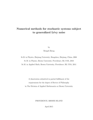
12. List of Figures
2.1 Empirical CDF of KL Expansion RVs Y1, ..., YM with M = 10 KL
expansion terms, for a centered Poisson process (Nt − λt) of λ =
10, Tmax = 1, with s = 10000 samples, and N = 200 points on the
time domain [0, 1]. . . . . . . . . . . . . . . . . . . . . . . . . . . . . 13
2.2 Exact sample path vs. sample path approximated by the KL ex-
pansion: when λ is smaller, the sample path is better approximated.
(Brownian motion is the limiting case for a centered poisson process
with very large birth rate.) . . . . . . . . . . . . . . . . . . . . . . . . 14
2.3 Exact mean vs. mean by KL expansion: when λ is larger, the KL
representation seems to be better. . . . . . . . . . . . . . . . . . . . . 14
2.4 Exact 2nd moment vs. 2nd moment by KL expansion with sampled
coefficients. The 2nd moments are not as well approximated as the
mean. . . . . . . . . . . . . . . . . . . . . . . . . . . . . . . . . . . . 14
3.1 Orthogonality defined in (3.27) with respect to the polynomial order
i up to 20 with Binomial distributions. . . . . . . . . . . . . . . . . . 32
3.2 CPU time to evaluate orthogonality for Binomial distributions. . . . . 33
3.3 Minimum polynomial order i (vertical axis) such that orth(i) is greater
than a threshold value. . . . . . . . . . . . . . . . . . . . . . . . . . . 34
3.4 Left: GENZ1 functions with different values of c and w; Right: h-
convergence of ME-PCM for function GENZ1. Two Gauss quadrature
points, d = 2, are employed in each element corresponding to a degree
m = 3 of exactness. c = 0.1, w = 1, ξ ∼ Bino(120, 1/2). Lanczos
method is employed to compute the orthogonal polynomials. . . . . . 42
3.5 Left: GENZ4 functions with different values of c and w; Right: h-
convergence of ME-PCM for function GENZ4. Two Gauss quadrature
points, d = 2, are employed in each element corresponding to a degree
m = 3 of exactness. c = 0.1, w = 1, ξ ∼ Bino(120, 1/2). Lanczos
method is employed for numerical orthogonality. . . . . . . . . . . . . 43
3.6 Non-nested sparse grid points with respect to sparseness parameter
k = 3, 4, 5, 6 for random variables ξ1, ξ2 ∼ Bino(10, 1/2), where the
one-dimensional quadrature formula is based on Gauss quadrature rule. 44
3.7 Convergence of sparse grids and tensor product grids to approximate
E[fi(ξ1, ξ2)], where ξ1 and ξ2 are two i.i.d. random variables associated
with a distribution Bino(10, 1/2). Left: f1 is GENZ1 Right: f4 is
GENZ4. Orthogonal polynomials are generated by Lanczos method. . 45
xii

13. 3.8 Convergence of sparse grids and tensor product grids to approximate
E[fi(ξ1, ξ2, ..., ξ8)], where ξ1,...,ξ8 are eight i.i.d. random variables asso-
ciated with a distribution Bino(10, 1/2). Left: f1 is GENZ1 Right: f4
is GENZ4. Orthogonal polynomials are generated by Lanczos method. 45
3.9 p-convergence of PCM with respect to errors defined in equations
(3.54) and (3.55) for the reaction equation with t = 1, y0 = 1. ξ is
associated with negative binomial distribution with c = 1
2
and β = 1.
Orthogonal polynomials are generated by the Stieltjes method. . . . . 47
3.10 Left: exact solution of the KdV equation (3.65) at time t = 0, 1.
Right: the pointwise error for the soliton at time t = 1 . . . . . . . . 49
3.11 p-convergence of PCM with respect to errors defined in equations
(3.67) and (3.68) for the KdV equation with t = 1. a = 1, x0 = −5
and σ = 0.2, with 200 Fourier collocation points on the spatial domain
[−30, 30]. Left: ξ ∼Pois(10); Right: ξ ∼ Bino(n = 5, p = 1/2)). aPC
stands for arbitrary Polynomial Chaos, which is Polynomial Chaos
with respect to arbitrary measure. Orthogonal polynomials are gen-
erated by Fischer’s method. . . . . . . . . . . . . . . . . . . . . . . . 50
3.12 h-convergence of ME-PCM with respect to errors defined in equations
(3.67) and (3.68) for the KdV equation with t = 1.05, a = 1, x0 = −5,
σ = 0.2, and ξ ∼ Bino(n = 120, p = 1/2), with 200 Fourier collocation
points on the spatial domain [−30, 30], where two collocation points
are employed in each element. Orthogonal polynomials are generated
by the Fischer method (left) and the Stieltjes method (right). . . . . 51
3.13 Adapted mesh with five elements with respect to Pois(40) distribution. 52
3.14 p-convergence of ME-PCM on a uniform mesh and an adapted mesh
with respect to errors defined in equations (3.67) and (3.68) for the
KdV equation with t = 1, a = 1, x0 = −5, σ = 0.2, and ξ ∼
Pois(40), with 200 Fourier collocation points on the spatial domain
[−30, 30]. Left: Errors of the mean. Right: Errors of the second
moment. Orthogonal polynomials are generated by the Nowak method. 53
3.15 ξ1, ξ2 ∼ Bino(10, 1/2): convergence of sparse grids and tensor product
grids with respect to errors defined in equations (3.67) and (3.68) for
problem (3.69), where t = 1, a = 1, x0 = −5, and σ1 = σ2 = 0.2,
with 200 Fourier collocation points on the spatial domain [−30, 30].
Orthogonal polynomials are generated by the Lanczos method. . . . 54
3.16 ξ1 ∼ Bino(10, 1/2) and ξ2 ∼ N(0, 1): convergence of sparse grids and
tensor product grids with respect to errors defined in in equations
(3.67) and (3.68) for problem (3.69), where t = 1, a = 1, x0 = −5,
and σ1 = σ2 = 0.2, with 200 Fourier collocation points on the spatial
domain [−30, 30]. Orthogonal polynomials are generated by Lanczos
method. . . . . . . . . . . . . . . . . . . . . . . . . . . . . . . . . . . 55
3.17 Convergence of sparse grids and tensor product grids with respect to
errors defined in in equations (3.67) and (3.68) for problem (3.70),
where t = 0.5, a = 0.5, x0 = −5, σi = 0.1 and ξi ∼ Bino(5, 1/2), i =
1, 2, ..., 8, with 300 Fourier collocation points on the spatial domain
[−50, 50]. Orthogonal polynomials are generated by Lanczos method. 56
xiii

14. 4.1 Reaction equation with one Poisson RV ξ ∼ Pois(λ) (d = 1): errors
versus final time T defined in (4.34) for different WM order Q in
equation (4.27), with polynomial order P = 10, y0 = 1, λ = 0.5. We
used RK4 scheme with time step dt = 1e − 4; k(ξ) = c0(ξ;λ)
2!
+ c1(ξ;λ)
3!
+
c2(ξ;λ)
4!
, σ = 0.1(left); k(ξ) = c0(ξ;λ)
0!
+ c1(ξ;λ)
3!
+ c2(ξ;λ)
6!
, σ = 1 (right). . . 68
4.2 Reaction equation with five Poisson RVs ξ1,...,5 ∼Pois(λ) (d = 5):
error defined in (4.34) with respect to time, for different WM order
Q, with parameters: λ = 1, σ = 0.5, y0 = 1, polynomial order P =
4, RK2 scheme with time step dt = 1e − 3, and k(ξ1, ξ2, ..., ξ5, t) =
5
i=1 cos(it)c1(ξi) in equation (4.23). . . . . . . . . . . . . . . . . . . 70
4.3 Reaction equation with one Poisson RV ξ1 ∼Pois(λ) and one Binomial
RV ξ2 ∼ Bino(N, p) (d = 2): error defined in (4.34) with respect to
time, for different WM order Q, with parameters: λ = 1, σ = 0.1,
N = 10, p = 1/2, y0 = 1, polynomial order P = 10, RK4 scheme with
time step dt = 1e − 4, and k(ξ1, ξ2, t) = c1(ξ1)k1(ξ2) in equation (4.23). 71
4.4 Burgers equation with one Poisson RV ξ ∼Pois(λ) (d = 1, ψ1(x, t) =
1): l2u2(T) error defined in (6.62) versus time, with respect to dif-
ferent WM order Q. Here we take in equation (4.32): polynomial
expansion order P = 6, λ = 1, ν = 1/2, σ = 0.1, IMEX (Crank-
Nicolson/RK2) scheme with time step dt = 2e − 4, and 100 Fourier
collocation points on [−π, π]. . . . . . . . . . . . . . . . . . . . . . . 73
4.5 P-convergence for Burgers equation with one Poisson RV ξ ∼Pois(λ)
(d = 1, ψ1(x, t) = 1): errors defined in equation (6.62) versus poly-
nomial expansion order P, for different WM order Q, and by prob-
abilistic collocation method (PCM) with P + 1 points with the fol-
lowing parameters: ν = 1, λ = 1, final time T = 0.5, IMEX (Crank-
Nicolson/RK2) scheme with time step dt = 5e − 4, 100 Fourier collo-
cation points on [−π, π], σ = 0.5 (left), and σ = 1 (right). . . . . . . 73
4.6 Q-convergence for Burgers equation with one Poisson RV ξ ∼Pois(λ)
(d = 1, ψ1(x, t) = 1): errors defined in equation (6.62) versus WM
order Q, for different polynomial order P, with the following param-
eters: ν = 1, λ = 1, final time T = 0.5, IMEX(RK2/Crank-Nicolson)
scheme with time step dt = 5e − 4, 100 Fourier collocation points on
[−π, π], σ = 0.5 (left), and σ = 1 (right). The dashed lines serve as a
reference of the convergence rate. . . . . . . . . . . . . . . . . . . . . 74
4.7 Burgers equation with three Poisson RVs ξ1,2,3 ∼Pois(λ) (d = 3): error
defined in equation (6.62) with respect to time, for different WM order
Q, with parameters: λ = 0.1, σ = 0.1, y0 = 1, ν = 1/100, polynomial
order P = 2, IMEX (RK2/Crank-Nicolson) scheme with time step
dt = 2.5e − 4. . . . . . . . . . . . . . . . . . . . . . . . . . . . . . . . 76
4.8 Reaction equation with P-adaptivity and two Poisson RVs ξ1,2 ∼Pois(λ)
(d = 2): error defined in (4.34) with two Poisson RVs by comput-
ing the WM propagator in equation (4.27) with respect to time by
the RK2 method with: fixed WM order Q = 1, y0 = 1, ξ1,2 ∼
Pois(1), a(ξ1, ξ2, t) = c1(ξ1; λ)c1(ξ2; λ), for fixed polynomial order
P (dashed lines), for varied polynomial order P (solid lines), for
σ = 0.1 (left), and σ = 1 (right). Adaptive criterion values are:
l2err(t) ≤ 1e − 8(left), and l2err(t) ≤ 1e − 6(right). . . . . . . . . . . 77
xiv

15. 4.9 Burgers equation with P-Q-adaptivity and one Poisson RV ξ ∼Pois(λ)
(d = 1, ψ1(x, t) = 1): error defined in equation (6.62) by comput-
ing the WM propagator in equation (4.32) with IMEX (RK2/Crank-
Nicolson) method (λ = 1, ν = 1/2, time step dt = 2e − 4). Fixed
polynomial order P = 6, σ = 1, and Q is varied (left); fixed WM
order Q = 3, σ = 0.1, and P is varied (right). Adaptive criterion
value is: l2u2(T) ≤ 1e − 10 (left and right). . . . . . . . . . . . . . . 78
4.10 Terms in Q
p=0
P
i=0 ˆui
∂ˆuk+2p−i
∂x
Ki,k+2p−i,p for each PDE in the WM
propagator for Burgers equation with one RV in equation (4.38) are
denoted by dots on the grids: here P = 4, Q = 1
2
, k = 0, 1, 2, 3, 4. Each
grid represents a PDE in the WM propagator, labeled by k. Each dot
represents a term in the sum Q
p=0
P
i=0 ˆui
∂ˆuk+2p−i
∂x
Ki,k+2p−i,p . The
small index next to the dot is for p, x direction is the index i for ˆui,
and y direction is the index k + 2p − i in
∂ˆuk+2p−i
∂x
. The dots on the
same diagonal line have the same index p. . . . . . . . . . . . . . . . 81
4.11 The total number of terms as ˆum1...md
∂
∂x
ˆuk1+2p1−m1,...,kd+2pd−md
Km1,k1+2p1−m1,p1
...Kmd,kd+2pd−md,pd
in the WM propagator for Burgers equation with d
RVs, as C(P, Q)d
: for dimensions d = 2 (left) and d = 3 (right). Here
we assume P1 = ... = Pd = P and Q1 = ... = Qd = Q. . . . . . . . . . 83
5.1 Empirical histograms of an IG subordinator (α = 1/2) simulated via
the CP approximationat t = 0.5: the IG subordinator has c = 1,
λ = 3; each simulation contains s = 106
samples (we zoom in and plot
x ∈ [0, 1.8] to examine the smaller jumps approximation); they are
with different jump truncation sizes as δ = 0.1 (left, dotted, CPU time
1450s), δ = 0.02 (middle, dotted, CPU time 5710s), and δ = 0.005
(right, dotted, CPU time 38531s). The reference PDFs are plotted in
red solid lines; the one-sample K-S test values are calculated for each
plot; the RelTol of integration in U(δ) and bδ
is 1 × 10−8
. These runs
were done on Intel (R) Core (TM) i5-3470 CPU @ 3.20 GHz in Matlab. 99
5.2 Empirical histograms of an IG subordinator (α = 1/2) simulated via
the series representationat t = 0.5: the IG subordinator has c = 1,
λ = 3; each simulation is done on the time domain [0, 0.5] and con-
tains s = 106
samples (we zoom in and plot x ∈ [0, 1.8] to examine
the smaller jumps approximation); they are with different number of
truncations in the series as Qs = 10 (left, dotted, CPU time 129s),
Qs = 100 (middle, dotted, CPU time 338s), and Qs = 1000 (right,
dotted, CPU time 2574s). The reference PDFs are plotted in red
solid lines; the one-sample K-S test values are calculated for each
plot. These runs were done on Intel (R) Core (TM) i5-3470 CPU @
3.20 GHz in Matlab. . . . . . . . . . . . . . . . . . . . . . . . . . . . 99
5.3 PCM/CP vs. PCM/S: error l2u2(T) of the solution for Equation (5.1)
versus the number of jumps Qcp (in PCM/CP) or Qs (in PCM/S)
with λ = 10 (left) and λ = 1 (right). T = 1, c = 0.1, α = 0.5,
= 0.1, µ = 2, Nx = 500 Fourier collocation points on [0, 2] (left
and right). In the PCM/CP: RelTol = 1 × 10−10
for integration
in U(δ). In the PCM/S: RelTol = 1 × 10−8
for the integration of
E[((
αΓj
2cT
)−1/α
∧ ηjξ
1/α
j )2
]. . . . . . . . . . . . . . . . . . . . . . . . . . 107
xv

16. 5.4 PCM vs. MC: error l2u2(T) of the solution for Equation (5.1) versus
the number of samples s obtained by MC/CP and PCM/CP with
δ = 0.01 (left) and MC/S with Qs = 10 and PCM/S (right). T = 1
, c = 0.1, α = 0.5, λ = 1, = 0.1, µ = 2 (left and right). Spatial
discretization: Nx = 500 Fourier collocation points on [0, 2] (left and
right); temporal discretization: first-order Euler scheme in (5.22) with
time steps t = 1 × 10−5
(left and right). In both MC/CP and
PCM/CP: RelTol = 1 × 10−8
for integration in U(δ). . . . . . . . . 109
5.5 Zoomed in density Pts(t, x) plots for the solution of Equation (5.2)
at different times obtained from solving Equation (5.37) for α = 0.5
(left) and Equation (5.42) for α = 1.5 (right): σ = 0.4, x0 = 1, c = 1,
λ = 10 (left); σ = 0.1, x0 = 1, c = 0.01, λ = 0.01 (right). We have
Nx = 2000 equidistant spatial points on [−12, 12] (left); Nx = 2000
points on [−20, 20] (right). Time step is t = 1 × 10−4
(left) and
t = 1 × 10−5
(right). The initial conditions are approximated by δD
20
(left and right). . . . . . . . . . . . . . . . . . . . . . . . . . . . . . 114
5.6 Density/CP vs. PCM/CP with the same δ: errors err1st and err2nd
of the solution for Equation (5.2) versus time obtained by the density
Equation (5.36) with CP approximation and PCM/CP in Equation
(5.55). c = 0.5, α = 0.95, λ = 10, σ = 0.01, x0 = 1 (left); c = 0.01,
α = 1.6, λ = 0.1, σ = 0.02, x0 = 1 (right). In the density/CP: RK2
with time steps t = 2 × 10−3
, 1000 Fourier collocation points on
[−12, 12] in space, δ = 0.012, RelTol = 1 × 10−8
for U(δ), and initial
condition as δD
20 (left and right). In the PCM/CP: the same δ = 0.012
as in the density/CP. . . . . . . . . . . . . . . . . . . . . . . . . . . 116
5.7 TFPDE vs. PCM/CP: error err2nd of the solution for Equation (5.2)
versus time with λ = 10 (left) and λ = 1 (right). Problems we are
solving: α = 0.5, c = 2, σ = 0.1, x0 = 1 (left and right). For
PCM/CP: RelTol = 1 × 10−8
for U(δ) (left and right). For the TF-
PDE: finite difference scheme in (5.47) with t = 2.5 × 10−5
, Nx
equidistant points on [−12, 12], initial condition given by δD
40 (left and
right). . . . . . . . . . . . . . . . . . . . . . . . . . . . . . . . . . . . 118
5.8 Zoomed in plots for the density Pts(x, T) by solving the TFPDE (5.37)
and the empirical histogram by MC/CP at T = 0.5 (left) and T = 1
(right): α = 0.5, c = 1, λ = 1, x0 = 1 and σ = 0.01 (left and
right). In the MC/CP: sample size s = 105
, 316 bins, δ = 0.01,
RelTol = 1 × 10−8
for U(δ), time step t = 1 × 10−3
(left and
right). In the TFPDE: finite difference scheme given in (5.47) with
t = 1 × 10−5
in time, Nx = 2000 equidistant points on [−12, 12]
in space, and the initial conditions are approximated by δD
40 (left and
right). We perform the one-sample K-S tests here to test how two
methods match. . . . . . . . . . . . . . . . . . . . . . . . . . . . . . 119
6.1 An illustration of the applications of multi-dimensional L´evy jump
models in mathematical finance. . . . . . . . . . . . . . . . . . . . . 127
6.2 Three ways to correlate L´evy pure jump processes. . . . . . . . . . . 128
6.3 The L´evy measures of bivariate tempered stable Clayton processes
with different dependence strength (described by the correlation length
τ) between their L1 and L2 components. . . . . . . . . . . . . . . . . 133
xvi

17. 6.4 The L´evy measures of bivariate tempered stable Clayton processes
with different dependence strength (described by the correlation length
τ) between their L++
1 and L++
2 components (only in the ++ corner).
It shows how the dependence structure changes with respect to the
parameter τ in the Clayton family of copulas. . . . . . . . . . . . . . 134
6.5 trajectory of component L++
1 (t) (in blue) and L++
2 (t) (in green) that
are dependent described by Clayton copula with dependent structure
parameter τ. Observe how trajectories get more similar when τ in-
creases. . . . . . . . . . . . . . . . . . . . . . . . . . . . . . . . . . . . 137
6.6 Sample path of (L1, L2) with marginal L´evy measure given by equation
(6.14), L´evy copula given by (6.13), with each components such as
F++
given by Clayton copula with parameter τ. Observe that when τ
is bigger, the ’flipping’ motion happens more symmetrically, because
there is equal chance for jumps to be the same sign with the same
size, and for jumps to be the opposite signs with the same size. . . . 139
6.7 Sample paths of bivariate tempered stable Clayton L´evy jump pro-
cesses (L1, L2) simulated by the series representation given in Equa-
tion (6.30). We simulate two sample paths for each value of τ. . . . . 140
6.8 An illustration of the three methods used in this paper to solve the
moment statistics of Equation (6.1). . . . . . . . . . . . . . . . . . . 140
6.9 An illustration of the three methods used in this paper to solve the
moment statistics of Equation (6.1). . . . . . . . . . . . . . . . . . . 147
6.10 An illustration of the three methods used in this paper to solve the
moment statistics of Equation (6.1). . . . . . . . . . . . . . . . . . . 148
6.11 PCM/S (probabilistic) vs. MC/S (probabilistic): error l2u2(t) of the
solution for Equation (6.1) with a bivariate pure jump L´evy process
with the L´evy measure in radial decomposition given by Equation
(6.9) versus the number of samples s obtained by MC/S and PCM/S
(left) and versus the number of collocation points per RV obtained
by PCM/S with a fixed number of truncations Q in Equation (6.10)
(right). t = 1 , c = 1, α = 0.5, λ = 5, µ = 0.01, NSR = 16.0%
(left and right). In MC/S: first order Euler scheme with time step
t = 1 × 10−3
(right). . . . . . . . . . . . . . . . . . . . . . . . . . . 151
6.12 PCM/series rep v.s. exact: T = 1. We test the noise/signal=variance/mean
ratio to be 4% at T = 1. . . . . . . . . . . . . . . . . . . . . . . . . . 152
6.13 PCM/series d-convergence and Q-convergence at T=1. We test the
noise/signal=variance/mean ratio to be 4% at t=1. The l2u2 error is
defined as l2u2(t) =
||Eex[u2(x,t;ω)]−Enum[u2(x,t;ω)]||L2([0,2])
||Eex[u2(x,t;ω)]||L2([0,2])
. . . . . . . . . . 153
6.14 MC v.s. exact: T = 1. Choice of parameters of this problem: we
evaluated the moment statistics numerically with integration rela-
tive tolerance to be 10−8
. With this set of parameter, we test the
noise/signal=variance/mean ratio to be 4% at T = 1. . . . . . . . . . 153
6.15 MC v.s. exact: T = 2. Choice of parameters of this problem: we
evaluated the moment statistics numerically with integration rela-
tive tolerance to be 10−8
. With this set of parameter, we test the
noise/signal=variance/mean ratio to be 10% at T = 2. . . . . . . . . 154
xvii

18. 6.16 FP (deterministic) vs. MC/S (probabilistic): joint PDF P(u1, u2, t)
of SODEs system in Equation (6.59) from FP Equation (6.41) (3D
contour plot), joint histogram by MC/S (2D contour plot on the x-
y plane), horizontal (subfigure) and vertical (subfigure) slices at the
peaks of density surface from FP equation and MC/S. Final time is
t = 1 (left, NSR = 16.0%) and t = 1.5 (right). c = 1, α = 0.5,
λ = 5, µ = 0.01. In MC/S: first-order Euler scheme with time step
t = 1×10−3
, 200 bins on both u1 and u2 directions, Q = 40, sample
size s = 106
. In FP: initial condition is given by MC data at t0 = 0.5,
RK2 scheme with time step t = 4 × 10−3
. . . . . . . . . . . . . . . . 155
6.17 TFPDE (deterministic) vs. PCM/S (probabilistic): error l2u2(t) of
the solution for Equation (6.1) with a bivariate pure jump L´evy pro-
cess with the L´evy measure in radial decomposition given by Equation
(6.9) obtained by PCM/S in Equation (6.64) (stochastic approach)
and TFPDE in Equation (6.41) (deterministic approach) versus time.
α = 0.5, λ = 5, µ = 0.001 (left and right). c = 0.1 (left); c = 1 (right).
In TFPDE: initial condition is given by δG
2000 in Equation (6.67), RK2
scheme with time step t = 4 × 10−3
. . . . . . . . . . . . . . . . . . 156
6.18 Exact mean, variance, and NSR versus time. The noise/signal ratio
is 10% at T = 0.5. . . . . . . . . . . . . . . . . . . . . . . . . . . . . . 160
6.19 PCM/S (probabilistic) vs. MC/S (stochastic): error l2u2(t) of the so-
lution for Equation (6.1) driven by a bivariate TS Clayton L´evy pro-
cess with L´evy measure given in Section 1.2.2 versus the number of
truncations Q in the series representation (6.32) by PCM/S (left) and
versus the number of samples s in MC/S with the series representation
(6.30) by computing Equation (6.59) (right). t = 1 , α = 0.5, λ = 5,
µ = 0.01, τ = 1 (left and right). c = 0.1, NSR = 10.1% (right). In
MC/S: first order Euler scheme with time step t = 1 × 10−2
(right). 162
6.20 Q-convergence (with various λ) of PCM/S in Equation (6.64):α = 0.5,
µ = 0.01, RelTol of integration of moments of jump sizes is 1e-8. . . . 162
6.21 FP (deterministic) vs. MC/S (probabilistic): joint PDF P(u1, u2, t)
of SODE system in Equation (6.59) from FP Equation (6.40) (three-
dimensional contour plot), joint histogram by MC/S (2D contour plot
on the x-y plane), horizontal (left, subfigure) and vertical (right, sub-
figure) slices at the peak of density surfaces from FP equation and
MC/S. Final time t = 1 (left) and t = 1.5 (right). c = 0.5, α = 0.5,
λ = 5, µ = 0.005, τ = 1 (left and right). In MC/S: first-order Eu-
ler scheme with time step t = 0.02, Q = 2 in series representation
(6.30), sample size s = 104
. 40 bins on both u1 and u2 directions
(left); 20 bins on both u1 and u2 directions (right). In FP: initial
condition is given by δG
1000 in Equation (6.67), RK2 scheme with time
step t = 4 × 10−3
. . . . . . . . . . . . . . . . . . . . . . . . . . . . . 164
6.22 TFPDE (deterministic) vs. PCM/S (stochastic): error l2u2(t) of the
solution for Equation (6.1) driven by a bivariate TS Clayton L´evy pro-
cess with L´evy measure given in Section 1.2.2 versus time obtained by
PCM/S in Equation (6.81) (stochastic approach) and TFPDE (6.40)
(deterministic approach). c = 1, α = 0.5, λ = 5, µ = 0.01 (left and
right). c = 0.05, µ = 0.001 (left). c = 1, µ = 0.005 (right). In
TFPDE: initial condition is given by δG
1000 in Equation (6.67), RK2
scheme with time step t = 4 × 10−3
. . . . . . . . . . . . . . . . . . 165
xviii

19. 6.23 S-convergence in MC/S with 10-dimensional L´evy jump processes:difference
in the E[u2
] (left) between different sample sizes s and s = 106
(as a
reference). The heat equation (6.1) is driven by a 10-dimensional jump
process with a L´evy measure (6.9) obtained by MC/S with series rep-
resentation (6.10). We show the L2 norm of these differences versus
s (right). Final time T = 1, c = 0.1, α = 0.5, λ = 10, µ = 0.01, time
step t = 4 × 10−3
, and Q = 10. The NSR at T = 1 is 6.62%. . . . . 167
6.24 Samples of (u1, u2) (left) and joint PDF of (u1, u2, ..., u10) on the
(u1, u2) plane by MC (right) : c = 0.1, α = 0.5, λ = 10, µ = 0.01,dt =
4e − 3 (first order Euler scheme), T = 1, Q = 10 (number of trunca-
tions in the series representation), and sample size s = 106
. . . . . . 167
6.25 Samples of (u9, u10) (left) and joint PDF of (u1, u2, ..., u10) on the
(u9, u10) plane by MC (right) : c = 0.1, α = 0.5, λ = 10, µ = 0.01,dt =
4e − 3 (first order Euler scheme), T = 1, Q = 10 (number of trunca-
tions in the series representation), and sample size s = 106
. . . . . . . 168
6.26 First two moments for solution of the heat equation (6.1) driven by a
10-dimensional jump process with a L´evy measure (6.9) obtained by
MC/S with series representation (6.10) at final time T = 0.5 (left) and
T = 1 (right) by MC : c = 0.1, α = 0.5, λ = 10, µ = 0.01, dt = 4e − 3
(with the first order Euler scheme), Q = 10, and sample size s = 106
. 169
6.27 Q-convergence in PCM/S with 10-dimensional L´evy jump processes:difference
in the E[u2
] (left) between different series truncation order Q and
Q = 16 (as a reference). The heat equation (6.1) is driven by a
10-dimensional jump process with a L´evy measure (6.9) obtained by
MC/S with series representation (6.10). We show the L2 norm of these
differences versus Q (right). Final time T = 1, c = 0.1, α = 0.5, λ =
10, µ = 0.01. The NSR at T = 1 is 6.62%. . . . . . . . . . . . . . . . 169
6.28 MC/S V.s. PCM/S with 10-dimensional L´evy jump processes:difference
between the E[u2
] computed from MC/S and that computed from
PCM/S at final time T = 0.5 (left) and T = 1 (right). The heat equa-
tion (6.1) is driven by a 10-dimensional jump process with a L´evy
measure (6.9) obtained by MC/S with series representation (6.10).
c = 0.1, α = 0.5, λ = 10, µ = 0.01. In MC/S, time step t = 4×10−3
,
Q = 10. In PCM/S, Q = 16. . . . . . . . . . . . . . . . . . . . . . . . 170
6.29 The function in Equation (6.82) with d = 2 (left up and left down)
and the ANOVA approximation of it with effective dimension of two
(right up and right down). A = 0.5, d = 2. . . . . . . . . . . . . . . . 173
6.30 The function in Equation (6.82) with d = 2 (left up and left down)
and the ANOVA approximation of it with effective dimension of two
(right up and right down). A = 0.1, d = 2. . . . . . . . . . . . . . . . 173
6.31 The function in Equation (6.82) with d = 2 (left up and left down)
and the ANOVA approximation of it with effective dimension of two
(right up and right down). A = 0.01, d = 2. . . . . . . . . . . . . . . 174
xix

20. 6.32 1D-ANOVA-FP V.s. 2D-ANOVA-FP with 10-dimensional L´evy jump processes:the
mean (left) for the solution of the heat equation (6.1) driven by a 10-
dimensional jump process with a L´evy measure (6.9) computed by
1D-ANOVA-FP, 2D-ANOVA-FP, and PCM/S. The L2 norms of dif-
ference in E[u] between these three methods are plotted versus final
time T (right). c = 1, α = 0.5, λ = 10, µ = 10−4
. In 1D-ANOVA-FP:
t = 4 × 10−3
in RK2, M = 30 elements, q = 4 GLL points on
each element. In 2D-ANOVA-FP: t = 4 × 10−3
in RK2, M = 5
elements on each direction, q2
= 16 GLL points on each element. In
PCM/S: Q = 10 in the series representation (6.10). Initial condition
of ANOVA-FP: MC/S data at t0 = 0.5, s = 1 × 104
, t = 4 × 10−3
.
NSR ≈ 18.24% at T = 1. . . . . . . . . . . . . . . . . . . . . . . . . 175
6.33 1D-ANOVA-FP V.s. 2D-ANOVA-FP with 10-dimensional L´evy jump processes:the
second moment (left) for the solution of heat equation (6.1) driven by
a 10-dimensional jump process with a L´evy measure (6.9) computed
by 1D-ANOVA-FP, 2D-ANOVA-FP, and PCM/S. The L2 norms of
difference in E[u2
] between these three methods are plotted versus
final time T (right). c = 1, α = 0.5, λ = 10, µ = 10−4
. In 1D-ANOVA-
FP: t = 4 × 10−3
in RK2, M = 30 elements, q = 4 GLL points
on each element. In 2D-ANOVA-FP: t = 4 × 10−3
in RK2, M = 5
elements on each direction, q2
= 16 GLL points on each element. Ini-
tial condition of ANOVA-FP: MC/S data at t0 = 0.5, s = 1 × 104
,
t = 4×10−3
. In PCM/S: Q = 10 in the series representation (6.10).
NSR ≈ 18.24% at T = 1. . . . . . . . . . . . . . . . . . . . . . . . . 176
6.34 Evolution of marginal distributions pi(xi, t) at final time t = 0.6, ..., 1.
c = 1 , α = 0.5, λ = 10, µ = 10−4
. Initial condition from MC:
t0 = 0.5, s = 104
, dt = 4 × 10−3
, Q = 10. 1D-ANOVA-FP : RK2
with time step dt = 4 × 10−3
, 30 elements with 4 GLL points on each
element . . . . . . . . . . . . . . . . . . . . . . . . . . . . . . . . . . 177
6.35 Showing the mean E[u] at different final time by PCM (Q = 10) and
by solving 1D-ANOVA-FP equations. c = 1 , α = 0.5, λ = 10,
µ = 1e − 4. Initial condition from MC: s = 104
, dt = 4−3
, Q = 10.
1D-ANOVA-FP : RK2 with dt = 4 × 10−3
, 30 elements with 4 GLL
points on each element. . . . . . . . . . . . . . . . . . . . . . . . . . 178
6.36 The mean E[u2
] at different final time by PCM (Q = 10) and by
solving 1D-ANOVA-FP equations. c = 1 , α = 0.5, λ = 10, µ = 1e−4.
Initial condition from MC: s = 104
, dt = 4 × 10−3
, Q = 10. 1D-
ANOVA-FP : RK2 with dt = 4 × 10−3
, 30 elements with 4 GLL
points on each element. . . . . . . . . . . . . . . . . . . . . . . . . . 179
6.37 The mean E[u2
] at different final time by PCM (Q = 10) and by
solving 2D-ANOVA-FP equations. c = 1 , α = 0.5, λ = 10, µ = 10−4
.
Initial condition from MC: s = 104
, dt = 4 × 10−3
, Q = 10. 2D-
ANOVA-FP : RK2 with dt = 4 × 10−3
, 30 elements with 4 GLL
points on each element. . . . . . . . . . . . . . . . . . . . . . . . . . 180
6.38 Left: sensitivity index defined in Equation (6.87) on each pair of
(i, j), j ≥ i. Right: sensitivity index defined in Equation (6.88) on
each pair of (i, j), j ≥ i. They are computed from the MC data at
t0 = 0.5 with s = 104
samples. . . . . . . . . . . . . . . . . . . . . . 182
xx

21. 6.39 Error growth by 2D-ANOVA-FP in different dimension d:the error growth
l2u1rel(T; t0) in E[u] defined in Equation (6.91) versus final time T
(left); the error growth l2u2rel(T; t0) in E[u2
] defined in Equation
(6.92) versus T (middle); l2u1rel(T = 1; t0) and l2u2rel(T = 1; t0)
versus dimension d (right). We consider the diffusion equation (6.1)
driven by a d-dimensional jump process with a L´evy measure (6.9)
computed by 2D-ANOVA-FP, and PCM/S. c = 1, α = 0.5, µ = 10−4
(left, middle, right). In Equation (6.49): t = 4 × 10−3
in RK2,
M = 30 elements, q = 4 GLL points on each element. In Equation
(6.50): t = 4 × 10−3
in RK2, M = 5 elements on each direction,
q2
= 16 GLL points on each element. Initial condition of ANOVA-FP:
MC/S data at t0 = 0.5, s = 1 × 104
, t = 4 × 10−3
, and Q = 16. In
PCM/S: Q = 16 in the series representation (6.10). NSR ≈ 20.5%
at T = 1 for all the dimensions d = 2, 4, 6, 10, 14, 18. These runs were
done on Intel (R) Core (TM) i5-3470 CPU @ 3.20 GHz in Matlab. . . 184
7.1 Summary of thesis . . . . . . . . . . . . . . . . . . . . . . . . . . . . 189
xxi

22. Chapter One
Introduction

23. 2
1.1 Motivation
Stochastic partial differential equations (SPDEs) are widely used for stochastic mod-
eling in diverse applications from physics, to engineering, biology and many other
fields, where the source of uncertainty includes random coefficients and stochastic
forcing. Our work is motivated by two things: application and shortcomings of past
work.
The source of uncertainty, practically, can be any non-Gaussian process. In many
cases, the random parameters are only observed at discrete values, which implies
that a discrete probability measure is more appropriate from the modeling point of
view. More generally, random processes with jumps are of fundamental importance in
stochastic modeling, e.g., stochastic-volatility jump-diffusion models in finance [171],
stochastic simulation algorithms for modeling diffusion, reaction and taxis in biol-
ogy [41], fluid models with jumps [158], quantum-jump models in physics [35], etc.
This serves as the motivation of our work on simulating SPDEs driven by discrete
random variables (RVs). Nonlinear SPDEs with discrete RVs and jump processes are
of practical use, since sources of stochastic excitations including uncertain parame-
ters and boundary/initial conditions are typically observed at discrete values. Many
complex systems of fundamental and industrial importance are significantly affected
by the underlying fluctuations/variations in random excitations, such as stochastic-
volatility jump-diffusion model in mathematical finance [12, 13, 24, 27, 28, 171],
stochastic simulation algorithms for modeling diffusion, reaction and taxis in biol-
ogy [41], truncated Levy flight model in turbulence [85, 106, 121, 158], quantum-jump
models in physics [35], etc.
An interesting source of uncertainty is L´evy jump processes, such as tempered

24. 3
α stable (TαS) processes. TαS processes were introduced in statistical physics to
model turbulence, e.g., the truncated L´evy flight model [85, 106, 121], and in math-
ematical finance to model stochastic volatility, e.g., the CGMY model [27, 28]. The
empirical distribution of asset prices is not always in a stable distribution or a nor-
mal distribution. The tail is heavier than a normal distribution and thinner than a
stable distribution [20]. Therefore, the TαS process was introduced as the CGMY
model to modify the Black and Scholes model. More details of white noise the-
ory for L´evy jump processes with applications to SPDEs and finance can be found
in [18, 120, 96, 97, 124]. Although one-dimensional (1D) jump models are constructed
in finance with L´evy processes [14, 86, 100], many financial models require multi-
dimensional L´evy jump processes with dependent components [33], such as basket
option pricing [94], portfolio optimization [39], and risk scenarios for portfolios [33].
In history, multi-dimensional Gaussian models are widely applied in finance because
of the simplicity in the description of dependence structures [134], however in some
applications we must take jumps in price processes into account [27, 28].
This work is constructed on previous work on the field of uncertainty quan-
tification (UQ), which includes the generalized polynomial chaos method (gPC),
multi-element generalized polynomial chaos method (MEgPC), probabilistic collo-
cation method (PCM), sparse collocation method, analysis of variance (ANOVA),
and many other variants (see, e.g., [8, 9, 50, 52, 58, 156] and references therein).
1.1.1 Computational limitations for UQ of nonlinear SPDEs
Numerically, nonlinear SPDEs with discrete processes are often solved by gPC in-
volving a system of coupled deterministic nonlinear equations [169], or probabilistic
collocation method (PCM) [50, 170, 177] involving nonlinear corresponding PDEs

25. 4
obtained at the collocation points. For stochastic processes with short correlation
length, the number of RVs required to represent the processes can be extremely large.
Therefore, the number of equations involved in the gPC propagator for a nonlinear
SPDE driven by such a process can be very large and highly coupled.
1.1.2 Computational limitations for UQ of SPDEs driven by
L´evy jump processes
For simulations of L´evy jump processes as TαS, we do not know the distribution of in-
crements explicitly [33], but we may still simulate the trajectories of TαS processes by
the random walk approximation [10]. However, the random walk approximation does
not identify the jump time and size of the large jumps precisely [139, 140, 141, 142].
In the heavy tailed case, large jumps contribute more than small jumps in functionals
of a L´evy process. Therefore, in this case, we have mainly used two other ways to
simulate the trajectories of a TαS process numerically: compound Poisson (CP) ap-
proximation [33] and series representation [140]. In the CP approximation, we treat
the jumps smaller than a certain size δ by their expectation, and treat the remaining
process with larger jumps as a CP process [33]. There are six different series represen-
tations of L´evy jump processes. They are the inverse L´evy measure method [44, 82],
LePage’s method [92], Bondesson’s method [23], thinning method [140], rejection
method [139], and shot noise method [140, 141]. However, in each representation,
the number of RVs involved is very large (such as 100). In this work, for TαS pro-
cesses, we will use the shot noise representation for Lt as a series representation
method because the tail of L´evy measure of a TαS process does not have an explicit
inverse [142]. Both the CP and the series approximation converge slowly when the
jumps of the L´evy process are highly concentrated around zero, however both can

26. 5
be improved by replacing the small jumps via Brownian motions [6]. The α-stable
distribution was introduced to model the empirical distribution of asset prices [104],
replacing the normal distribution. In the past literature, the simulation of SDEs or
functionals of TαS processes was mainly done via MC [128]. MC for functionals of
TαS processes is possible after a change of measure that transform TαS processes
into stable processes [130].
1.2 Introduction of TαS L´evy jump processes
TαS processes were introduced in statistical physics to model turbulence, e.g., the
truncated L´evy flight model [85, 106, 121], and in mathematical finance to model
stochastic volatility, e.g., the CGMY model [27, 28]. Here, we consider a symmet-
ric TαS process (Lt) as a pure jump L´evy martingale with characteristic triplet
(0, ν, 0) [19, 143] (no drift and no Gaussian part). The L´evy measure is given by [33]
1
:
ν(x) =
ce−λ|x|
|x|α+1
, 0 < α < 2. (1.1)
This L´evy measure can be interpreted as an Esscher transformation [57] from that
of a stable process with exponential tilting of the L´evy measure. The parameter
c > 0 alters the intensity of jumps of all given sizes; it changes the time scale of
the process. Also, λ > 0 fixes the decay rate of big jumps, while α determines the
relative importance of smaller jumps in the path of the process2
. The probability
density for Lt at a given time is not available in a closed form (except when α = 1
2
3
).
1
In a more generalized form, L´evy measure is ν(x) = c−e−λ−|x|
|x|α+1 Ix<0 + c+e−λ+|x|
|x|α+1 Ix>0. We may
have different coefficients c+, c−, λ+, λ− on the positive and the negative jump parts.
2
In the case when α = 0, Lt is the gamma process.
3
See inverse Gaussian processes.

27. 6
The characteristic exponent for Lt is [33]:
Φ(s) = s−1
log E[eisLs
] = 2Γ(−α)λα
c[(1 −
is
λ
)α
− 1 +
isα
λ
], α = 1, (1.2)
where Γ(x) is the Gamma function and E is the expectation. By taking the deriva-
tives of the characteristic exponent we obtain the mean and variance:
E[Lt] = 0, V ar[Lt] = 2tΓ(2 − α)cλα−2
. (1.3)
In order to derive the second moments for the exact solutions of Equations (5.1) and
(5.2), we introduce the Itˆo isometry. The jump of Lt is defined by Lt = Lt − Lt− .
We define the Poisson random measure N(t, U) as [71, 119, 123]:
N(t, U) =
0≤s≤t
I Ls∈U , U ∈ B(R0), ¯U ⊂ R0. (1.4)
Here R0 = R{0}, and B(R0) is the σ-algebra generated by the family of all Borel
subsets U ⊂ R, such that ¯U ⊂ R0; IA is an indicator function. The Poisson random
measure N(t, U) counts the number of jumps of size Ls ∈ U at time t. In order
to introduce the Itˆo isometry, we define the compensated Poisson random measure
˜N [71] as:
˜N(dt, dz) = N(dt, dz) − ν(dz)dt = N(dt, dz) − E[N(dt, dz)]. (1.5)
The TαS process Lt (as a martingale) can be also written as:
Lt =
t
0 R0
z ˜N(dτ, dz). (1.6)
For any t, let Ft be the σ-algebra generated by (Lt, ˜N(ds, dz)), z ∈ R0, s ≤ t. We
define the filtration to be F = {Ft, t ≥ 0}. If a stochastic process θt(z), t ≥ 0, z ∈ R0

28. 7
is Ft-adapted, we have the following Itˆo isometry [119]:
E[(
T
0 R0
θt(z) ˜N(dt, dz))2
] = E[
T
0 R0
θ2
t (z)ν(dz)dt]. (1.7)
1.3 Organization of the thesis
In Chapter 2, we discuss four methods to simulate L´evy jump processes preliminar-
ies and background information to the reader: 1. random walk approximation; 2.
Karhumen-Loeve expansion; 3. compound Poisson approximation; 4. series repre-
sentation.
In Chapter 3, The methods of generating orthogonal polynomial bases with re-
spect to discrete measures are presented, followed by a discussion about the error of
numerical integration. Numerical solutions of the stochastic reaction equation and
Korteweg- de Vries (KdV) equation, including adaptive procedures, are explained.
Then, we summarize the work. In the appendices, we provide more details about
the deterministic KdV equation solver, and the adaptive procedure.
In Chapter 4, we define the WM expansion and derive the Wick-Malliavin prop-
agators for a stochastic reaction equation and a stochastic Burgers equation. We
present several numerical results for SPDEs with one RV and multiple RVs, in-
cluding an adaptive procedure to control the error in time. We also compare the
computational complexity between gPC and WM for stochastic Burgers equation
with the same level of accuracy. Also, we provide an iterative algorithm to generate
coefficients in the WM approximation.
In Chapter 5, we compare the CP approximation and the series representation

29. 8
of a TαS process. We solve a stochastic reaction-diffusion with TαS white noise via
MC and PCM, both with CP approximation or series representation of the TαS pro-
cess. We simulate the density evolution for an overdamped Langevin equation with
TαS white noise via the corresponding generalized FP equations. We compare the
statistics obtained from the FP equations and MC or PCM methods. We conclude.
Also, we provide algorithms of the rejection method and simulation of CP processes.
We also provide the probability distributions to simplify the series representation.
In Chapter 6, by MC, PCM and FP, we solve the moment statistics for the solu-
tion of a heat equation driven by a 2D L´evy noise in LePage’s series representation.
By MC, PCM and FP, we solve the moment statistics for the solution of a heat equa-
tion driven by a 2D L´evy noise described by L´evy copula as. By MC, PCM and FP,
we solve the moment statistics for the solution of the heat equation driven by a 10D
L´evy noise in LePage’s series representation, where the FP equation is decomposed
by the unanchored ANOVA decomposition. We also exam the error growth versus
the dimension of the L´evy process. We conclude. Also, we show how we simplify the
multi-dimensional integration in FP equations into the 1D and 2D integrals.
In Chapter 7, lastly, we summarize the scope of SPDEs, the scope of stochastic
processes, and the methods we have experimented so far. We summarize the compu-
tational cost and accuracy in our numerical experiments. We suggest feasible future
works on methodology and applications.

30. Chapter Two
Simulation of L´evy jump processes

31. 10
In general there are three ways to generate a L´evy process [140]: random walk ap-
proximation, series representation and compound Poisson (CP) approximation. The
random walk approximation approximate the continuous random walk by a discrete
random walk on a discrete time sequence, if the marginal distribution of the process is
known. It is often used to simulate L´evy jump processes with large jumps, but it does
not identify the jump time and size of the large jumps precisely [139, 140, 141, 142].
We attempt to simulate a non-Gaussian process by Karhumen-Lo`eve (KL) expansion
here as well by computing the covariance kernel and its eigenfunctions. In the CP
approximation, we treat the jumps smaller than a certain size by their expectation
as a drift term, and the remaining process with large jumps as a CP process [33].
There are six different series representations of L´evy jump processes. They are the in-
verse L´evy measure method [44, 82], LePage’s method [92], Bondesson’s method [23],
thinning method [140], rejection method [139], and shot noise method [140, 141].
2.1 Random walk approximation to Poisson pro-
cesses
For a L´evy jump process Lt, on a fixed time grid [t0, t1, t2, ..., tN ], we may approximate
Lt by Lt = N
i=1 XiI{t < ti}. When the marginal distribution of Lt is known,
the distribution of Xi is known to be Lti−ti−1
. Therefore, on the fixed time grid,
we may generate the RVs Xi by sampling from the known distribution. When Lt
is composed of large jumps with low intensity (or rate of jumps), this can be a
good approximation. However, we are mostly interested in L´evy jump processes
with infinite activity (with high rates of jumps), therefore this will not be a good
approximation for the kind of processes we are going to consider, such as tempered

32. 11
α stable processes.
2.2 KL expansion for Poisson processes
Let us first take a Poisson process N(t; ω) with intensity λ on a computational time
domain [0, T] as an example. We mimic the KL expansion for Gaussian processes to
simulate non-Gaussian processes as Poisson processes.
• First we calculate the covariance kernel (assuming t > t).
Cov(N(t; ω)N(t ; ω)) = E[N(t; ω)N(t ; ω)] − E[N(t; ω)]E[N(t ; ω)]
= E[N(t; ω)N(t; ω)] + E[N(t; ω)]E[N(t − t; ω)] − E[N(t; ω)]E[N(t ; ω)]
= λt, t > t,
(2.1)
Therefore, the covariance kernel is
Cov(N(t; ω)N(t ; ω)) = λ(t t ) (2.2)
• The eigenvalues and eigenfunctions for this kernel would be:
ek(t) =
√
2sin(k −
1
2
)πt (2.3)
and
λk =
1
(k − 1
2
)2π2
(2.4)
where k=1,2,3,...
• The stochastic process Nt approximated by finite number of terms in the KL

33. 12
expansion can be written as:
˜N(t; ω) = λt +
M
i=1
λiYiei(t) (2.5)
where
1
0
e2
k(t)dt = 1 (2.6)
and
T
0
e2
k(t)dt = T −
sin[T(1 − 2k)π]
π(1 − 2k)
(2.7)
and they are orthogonal.
• The distribution of Yk can be calculated by the following. Given a sample path
ω ∈ Ω,
< N(t; ω) − λt, ek(t) >=
Yk
√
λ
π(k − 1
2
)
< ek(t), ek(t) >
= 2Yk
√
λ[
T(2k − 1)π − sin((2k − 1)πT)
π2(2k − 1)2
]
=< N(t; ω), ek(t) > −
√
2λ
π2
[−2πTcos(πT/2) + 4sin(πT/2)].
(2.8)
Therefore,
Yk =
π2
(2k − 1)2
[< N(t; ω), ek(t) > −
√
2λ
π2 [−2πTcos(πT/2) + 4sin(πT/2)]]
2
√
λ[T(2k − 1)π − sin((2k − 1)πT]
.
(2.9)
From each sample path each sample path ω, we can calculate the value of
Y1, ..., YM . In this way the distribution of Y1, ..., YM can be sampled. Nu-
merically, if we simulate enough number of samples of a Poisson process (by
simulating the jump times and jump sizes separately), we may have the em-
pirical distribution of RVs Y1, ..., YM .
• Now let us see how well the sample paths of the Poisson process Nt are ap-

34. 13
5 4 3 2 1 0 1 2 3 4 5
0
0.1
0.2
0.3
0.4
0.5
0.6
0.7
0.8
0.9
1
Empirical CDF for KL Exp RVs
i
CDF
Figure 2.1: Empirical CDF of KL Expansion RVs Y1, ..., YM with M = 10 KL expansion terms,
for a centered Poisson process (Nt −λt) of λ = 10, Tmax = 1, with s = 10000 samples, and N = 200
points on the time domain [0, 1].
proximated by the KL expansion.
• Now let us see how well the mean of the Poisson process Nt are approximated
by the KL expansion.
• Now let us see how well the second moment of the Poisson process Nt are
approximated by the KL expansion.
2.3 Compound Poisson approximation to L´evy jump
processes
Let us take a tempered α stable process (TαS) as an example here. TαS processes
were introduced in statistical physics to model turbulence, e.g., the truncated L´evy
flight model [85, 106, 121], and in mathematical finance to model stochastic volatility,
e.g., the CGMY model [27, 28]. Here, we consider a symmetric TαS process (Lt) as
a pure jump L´evy martingale with characteristic triplet (0, ν, 0) [19, 143] (no drift

35. 14
0 1 2 3 4 5
100
50
0
50
100
150
200
250
300
Exact and Approx ed Sample Path by KL Exp
time
N(t;0
)
ex sample path
approx ed sample path
10 Exp Terms
=50
T
max
=5
0 1 2 3 4 5
1
0
1
2
3
4
5
6
Exact and Approx ed Sample Path by KL Exp
time
N(t;0
)
exact sample path
approx ed sample path
10 Exp Terms
=1
T
max
=5
Figure 2.2: Exact sample path vs. sample path approximated by the KL expansion: when λ
is smaller, the sample path is better approximated. (Brownian motion is the limiting case for a
centered poisson process with very large birth rate.)
0 1 2 3 4 5
50
0
50
100
150
200
250
300
Mean Rep by KL Exp w/ Sampled Coefficients
time
<N(t;)>
Exact
KL Exp
10 Exp Terms
=50
T
max
=5
200 Samples
0 1 2 3 4 5
6
4
2
0
2
4
6
8
10
Mean Rep by KL Exp w/ Sampled Coefficients
time
<N(t;)>
Exact
KL Exp
10 Exp Terms
=1
T
max
=5
200 Samples
Figure 2.3: Exact mean vs. mean by KL expansion: when λ is larger, the KL representation
seems to be better.
0 1 2 3 4 5
0
1
2
3
4
5
6
7
x 10
4 2nd Moment Rep by KL Exp w/ Sampled Coefficients
time
<N2
(t;)>
Exact
KL Exp
10 Exp Terms
=50
T
max
=5
200 Samples
0 1 2 3 4 5
0
10
20
30
40
50
60
2nd Moment Rep by KL Exp w/ Sampled Coefficients
Time
<N2
(t;)>
Exact
KL Exp
10 Exp Terms
=1
T
max
=5
200 Samples
Figure 2.4: Exact 2nd moment vs. 2nd moment by KL expansion with sampled coefficients. The
2nd moments are not as well approximated as the mean.

36. 15
and no Gaussian part). The L´evy measure is given by [33] 1
:
ν(x) =
ce−λ|x|
|x|α+1
, 0 < α < 2. (2.10)
This L´evy measure can be interpreted as an Esscher transformation [57] from that
of a stable process with exponential tilting of the L´evy measure. The parameter
c > 0 alters the intensity of jumps of all given sizes; it changes the time scale of
the process. Also, λ > 0 fixes the decay rate of big jumps, while α determines the
relative importance of smaller jumps in the path of the process2
. The probability
density for Lt at a given time is not available in a closed form (except when α = 1
2
3
).
The characteristic exponent for Lt is [33]:
Φ(s) = s−1
log E[eisLs
] = 2Γ(−α)λα
c[(1 −
is
λ
)α
− 1 +
isα
λ
], α = 1, (2.11)
where Γ(x) is the Gamma function and E is the expectation. By taking the deriva-
tives of the characteristic exponent we obtain the mean and variance:
E[Lt] = 0, V ar[Lt] = 2tΓ(2 − α)cλα−2
. (2.12)
In the CP approximation, we simulate the jumps larger than δ as a CP process
and replace jumps smaller than δ by their expectation as a drift term [33]. Here
we explain the method to approximate a TαS subordinator Xt (without a Gaussian
part and a drift) with the L´evy measure ν(x) = ce−λx
xα+1 Ix>0 (positive jumps only); this
method can be generalized to a TαS process with both positive and negative jumps.
1
In a more generalized form, L´evy measure is ν(x) = c−e−λ−|x|
|x|α+1 Ix<0 + c+e−λ+|x|
|x|α+1 Ix>0. We may
have different coefficients c+, c−, λ+, λ− on the positive and the negative jump parts.
2
In the case when α = 0, Lt is the gamma process.
3
See inverse Gaussian processes.

37. 16
The CP approximation Xδ
t for this TαS subordinator Xt is:
Xt ≈ Xδ
t =
s≤t
XsI Xs≥δ+E[
s≤t
XsI Xs<δ] =
∞
i=1
Jδ
i It≤Ti
+bδ
t ≈
Qcp
i=1
Jδ
i It≤Ti
+bδ
t,
(2.13)
We introduce Qcp here as the number of jumps occurred before time t. The first
term ∞
i=1 Jδ
i It≤Ti
is a compound Poisson process with jump intensity
U(δ) = c
∞
δ
e−λx
dx
xα+1
(2.14)
and jump size distribution pδ
(x) = 1
U(δ)
ce−λx
xα+1 Ix≥δ for Jδ
i . The jump size random
variables (RVs) Jδ
i are generated via the rejection method [37]. This is the algorithm
of rejection method to generate RVs with distribution pδ
(x) = 1
U(δ)
ceλx
xα+1 Ix≥δ for CP
approximation [37]
The distribution pδ
(x) can be bounded by
pδ
(x) ≤
δ−α
e−λδ
αU(δ)
fδ
(x), (2.15)
where fδ
(x) = αδ−α
xα+1 Ix≥δ. The algorithm to generate RVs with distribution pδ
(x) =
1
U(δ)
ceλx
xα+1 Ix≥δ is [33, 37]:
• REPEAT
• Generate RVs W and V : independent and uniformly distributed on [0, 1]
• Set X = δW−1/α

38. 17
• Set T = fδ(X)δ−αe−λδ
pδ(X)αU(δ)
• UNTIL V T ≤ 1
• RETURN X .
Here, Ti is the i-th jump arrival time of a Poisson process with intensity U(δ).
The accuracy of CP approximation method can be improved by replacing the smaller
jumps by a Brownian motion [6], when the growth of the L´evy measure near zero
is fast. The second term functions as a drift term, bδ
t, resulted from truncating
the smaller jumps. The drift is bδ
= c
δ
0
e−λxdx
xα . This integration diverges when
α ≥ 1, therefore the CP approximation method only applies to TαS processes with
0 < α < 1. In this paper, both the intensity U(δ) and drift bδ
are calculated
via numerical integrations with Gauss-quadrature rules [54] with a specified relative
tolerance (RelTol) 4
. In general, there are two algorithms to simulate a compound
Poisson process [33]: the first method is to simulate the jump time Ti by exponentially
distributed RVs and take the number of jumps Qcp as large as possible; the second
method is to first generate and fix the number of jumps, then generate the jump time
by uniformly distributed RVs on [0, t]. Algorithms for simulating a CP process (the
second kind) with intensity and the jump size distribution in their explicit forms are
known on a fixed time grid [33]. Here we describe how to simulate the trajectories of a
CP process with intensity U(δ) and jump size distribution νδ(x)
U(δ)
, on a simulation time
domain [0, T] at time t. The algorithm to generate sample paths for CP processes
without a drift:
4
The RelTol of numerical integration is defined as |q−Q|
|Q| , where q is the computed value of the
integral and Q is the unknown exact value.

39. 18
• Simulate an RV N from Poisson distribution with parameter U(δ)T, as the
total number of jumps on the interval [0, T].
• Simulate N independent RVs, Ti, uniformly distributed on the interval [0, T],
as jump times.
• Simulate N jump sizes, Yi with distribution νδ(x)
U(δ)
.
• Then the trajectory at time t is given by N
i=1 ITi≤tYi.
In order to simulate the sample paths of a symmetric TαS process with a L´evy
measure given in Equation (5.3), we generate two independent TαS subordinators
via the CP approximation and subtract one from the other. The accuracy of the CP
approximation is determined by the jump truncation size δ.
The numerical experiments for this method will be given in Chapter 5.
2.4 Series representation to L´evy jump processes
Let { j}, {ηj}, and {ξj} be sequences of i.i.d. RVs such that P( j = ±1) = 1/2, ηj ∼
Exponential(λ), and ξj ∼Uniform(0, 1). Let {Γj} be arrival times in a Poisson
process with rate one. Let {Uj} be i.i.d. uniform RVs on [0, T]. Then, a TαS
process Lt with L´evy measure given in Equation (5.3) can be represented as [142]:
Lt =
+∞
j=1
j[(
αΓj
2cT
)−1/α
∧ ηjξ
1/α
j ]I{Uj≤t}, 0 ≤ t ≤ T. (2.16)
Equation (5.14) converges almost surely as uniformly in t [139]. In numerical simu-
lations, we truncate the series in Equation (5.14) up to Qs terms. The accuracy of

40. 19
series representation approximation is determined by the number of truncations Qs.
The numerical experiments for this method will be given in Chapter 5.

41. Chapter Three
Adaptive multi-element
polynomial chaos with discrete
measure: Algorithms and
applications to SPDEs

42. 21
We develop a multi-element probabilistic collocation method (ME-PCM) for arbi-
trary discrete probability measures with finite moments and apply it to solve partial
differential equations with random parameters. The method is based on numeri-
cal construction of orthogonal polynomial bases in terms of a discrete probability
measure. To this end, we compare the accuracy and efficiency of five different con-
structions. We develop an adaptive procedure for decomposition of the parametric
space using the local variance criterion. We then couple the ME-PCM with sparse
grids to study the Korteweg-de Vries (KdV) equation subject to random excitation,
where the random parameters are associated with either a discrete or a continuous
probability measure. Numerical experiments demonstrate that the proposed algo-
rithms lead to high accuracy and efficiency for hybrid (discrete-continuous) random
inputs.
3.1 Notation
µ, ν probability measure of discrete RVs
ξ discrete RV
Pi(ξ) generalized Polynomial Chaos basis function
δij Dirac delta function
S(µ) support of measure µ over discrete RV ξ
N size of the support S(µ)
αi, βi coefficients in the three term recurrence relation of orthogonal polynomial basis
mk the kith moment of RV ξ
Γ integration domain of the discrete RV
Wm,p
(Γ) Sobolev space
h size of element in multi-element integration
Nes number of elements in multi-element integration
d number of quadrature points in Gauss quadrature rule
Bi i-th element in the multi-element integration
σ2
i local variance

43. 22
3.2 Generation of orthogonal polynomials for dis-
crete measures
Let µ be a positive measure with infinite support S(µ) ⊂ R and finite moments at
all orders, i.e.,
S
ξn
µ(dξ) < ∞, ∀n ∈ N0, (3.1)
where N0 = {0, 1, 2, ...}, and it is defined as a Riemann-Stieltjes integral. There
exists one unique [54] set of orthogonal monic polynomials {Pi}∞
i=0 with respect to
the measure µ such that
S
Pi(ξ)Pj(ξ)µ(dξ) = δijγ−2
i , i = 0, 1, 2, . . . , (3.2)
where γi = 0 are constants. In particular, the orthogonal polynomials satisfy a
three-term recurrence relation [31, 43]
Pi+1(ξ) = (ξ − αi)Pi(ξ) − βiPi−1(ξ), i = 0, 1, 2, . . . (3.3)
The uniqueness of the set of orthogonal polynomials with respect to µ can be also
derived by constructing such set of polynomials starting from P0(ξ) = 1. We typ-
ically choose P−1(ξ) = 0 and β0 to be a constant. Then the full set of orthogonal
polynomials is completely determined by the coefficients αi and βi.
If the support S(µ) is a finite set with data points {τ1, ..., τN }, i.e., µ is a discrete
measure defined as
µ =
N
i=1
λiδτi
, λi > 0, (3.4)

44. 23
the corresponding orthogonality condition is finite, up to order N − 1 [46, 54], i.e.,
S
P2
i (ξ)µ(dξ) = 0, i ≥ N, (3.5)
where δτi
indicates the empirical measure at τi, although by the recurrence relation
(3.3) we can generate polynomials at any order greater than N − 1. Furthermore,
one way to test whether the coefficients αi are well approximated is to check the
following relation [45, 46]
N−1
i=0
αi =
N
i=1
τi. (3.6)
One can prove that the coefficient of ξN−1
in PN (ξ) is − N−1
i=0 αi, and PN (ξ) =
(ξ − τ1)...(ξ − τN ), therefore equation (3.6) holds [46].
We subsequently examine five different approaches of generating orthogonal poly-
nomials for a discrete measure and point out the pros and cons of each method. In
Nowak method, the coefficients of the polynomials are directly derived from solving
a linear system; in the other four methods, we generate coefficients αi and βi by four
different numerical methods, and the coefficients of polynomials are derived from the
recurrence relation in equation (3.3).
3.2.1 Nowak method
Define the k-th order moment as
mk =
S
ξk
µ(dξ), k = 0, 1, ..., 2d − 1. (3.7)

45. 24
The coefficients of the d-th order polynomial Pd(ξ) = d
i=0 aiξi
are determined by
the following linear system [125]












m0 m1 . . . md
m1 m2 . . . md+1
. . . . . . . . . . . .
md−1 md . . . m2d−1
0 0 . . . 1
























a0
a1
. . .
ad−1
ad












=












0
0
. . .
0
1












, (3.8)
where the (d + 1) by (d + 1) Vandermonde matrix needs to be inverted.
Although this method is straightforward to implement, it is well known that the
matrix may be ill conditioned when d is very large.
The total computational complexity for solving the linear system in equation
(3.8) is O(d2
) to generate Pd(ξ) 1
.
3.2.2 Stieltjes method
Stieltjes method is based on the following formulas of the coefficients αi and βi [54]
αi = S
ξP2
i (ξ)µ(dξ)
S
P2
i (ξ)µ(dξ)
, βi = S
ξP2
i (ξ)µ(dξ)
S
P2
i−1(ξ)µ(dξ)
, i = 0, 1, .., d − 1. (3.9)
For a discrete measure, the Stieltjes method is quite stable [54, 51]. When the
discrete measure has a finite number of elements in its support (N), the above
formulas are exact. However, if we use Stieltjes method on a discrete measure with
infinite support, i.e. Poisson distribution, we approximate the measure by a discrete
1
Here we notice that the Vandermonde matrix is in a Toeplitz matrix form. Therefore the
computational complexity of solving this linear system is O(d2
) [59, 157].

46. 25
measure with finite number of points; therefore, each time when we iterate for αi
and βi, the error accumulates by neglecting the points with less weights. In that
case, αi and βi may suffer from inaccuracy when i is close to N [54].
The computational complexity for integral evaluation in equation (3.9) is of the
order O(N).
3.2.3 Fischer method
Fischer proposed a procedure for generating the coefficients αi and βi by adding
data points one-by-one [45, 46]. Assume that the coefficients αi and βi are known
for the discrete measure µ = N
i=1 λiδτi
. Then, if we add another data point τ to
the discrete measure µ and define a new discrete measure ν = µ + λδτ , λ being the
weight of the newly added data point τ, the following relations hold [45, 46]:
αν
i = αi + λ
γ2
i Pi(τ)Pi+1(τ)
1 + λ i
j=0 γ2
j P2
j (τ)
− λ
γ2
i−1Pi(τ)Pi−1(τ)
1 + λ i−1
j=0 γ2
j P2
j (τ)
(3.10)
βν
i = βi
[1 + λ i−2
j=0 γ2
j P2
j (τ)][1 + λ i
j=0 γ2
j P2
j (τ)]
[1 + λ i−1
j=0 γ2
j P2
j (τ)]2
(3.11)
for i < N, and
αν
N = τ − λ
γ2
N−1PN (τ)PN−1(τ)
1 + λ N−1
j=0 γ2
j P2
j (τ)
(3.12)
βν
N =
λγ2
N−1P2
N (τ)[1 + λ N−2
j=0 γ2
j P2
j (τ)]
[1 + λ N−1
j=0 γ2
j P2
j (τ)]2
, (3.13)
where αν
i and βν
i indicate the coefficients in the three-term recurrence formula (3.3)
for the measure ν. The numerical stability of this algorithm depends on the stability
of the recurrence relations above, and on the sequence of data points added [46]. For

47. 26
example, the data points can be in either ascending or descending order. Fischer’s
method basically modifies the available coefficients αi and βi using the information
induced by the new data point. Thus, this approach is very practical when an
empirical distribution for stochastic inputs is altered by an additional possible value.
For example, let us consider that we have already generated d probability collocation
points with respect to the given discrete measure with N data points, and we want
to add another data point into the discrete measure to generate d new probability
collocation points with respect to the new measure. Using the Nowak method, we
will need to reconstruct the moment matrix and invert the matrix again with N + 1
data points; however by Fischer’s method, we will only need to update 2d values of
αi and βi by adding this new data point, which is more convenient.
We generate a new sequence of {αi, βi} by adding a new data point into the
measure, therefore the computational complexity for calculating the coefficients
{γ2
i , i = 0, .., d} for N times is O(N2
).
3.2.4 Modified Chebyshev method
Compared to the Chebyshev method [54], the modified Chebyshev method computes
moments in a different way. Define the quantities:
µi,j =
S
Pi(ξ)ξj
µ(dξ), i, j = 0, 1, 2, ... (3.14)
Then, the coefficients αi and βi satisfy [54]:
α0 =
µ0,1
µ0,0
, β0 = µ0,0, αi =
µi,i+1
µi,i
−
µi−1,i
µi−1,i−1
, βi =
µi,i
µi−1,i−1
. (3.15)

48. 27
Note that due to the orthogonality, µi,j = 0 when i > j. Starting from the moments
µj, µi,j can be computed recursively as
µi,j = µi−1,j+1 − αi−1µi−1,j − βi−1µi−2,j, (3.16)
with
µ−1,0 = 0, µ0,j = µj, (3.17)
where j = i, i + 1, ..., 2d − i − 1.
However, this method suffers from the same effects of ill-conditioning as the
Nowak method [125] does, because they both rely on calculating moments. To sta-
bilize the algorithm we introduce another way of defining moments by polynomials:
ˆµi,j =
S
Pi(ξ)pj(ξ)µ(dξ), (3.18)
where {pi(ξ)} is chosen to be a set of orthogonal polynomials, e.g., Legendre poly-
nomials. Define
νi =
S
pi(ξ)µ(dξ). (3.19)
Since {pi(ξ)}∞
i=0 is not a set of orthogonal polynomials with respect to the measure
µ(dξ), νi is, in general, not equal to zero. For all the following numerical experiments
we used the Legendre polynomials for {pi(ξ)}∞
i=0.2
Let ˆαi and ˆβi be the coefficients
in the three-term recurrence formula associated with the set {pi} of orthogonal poly-
nomials.
2
Legendre polynomials {pi(ξ)}∞
i=0 are defined on [−1, 1], therefore in implementation of the
Modified Chebyshev method, we scale the measure onto [−1, 1] first.

49. 28
Then, we initialize the process of building up the coefficients as
ˆµ−1,j = 0, j = 1, 2, ..., 2d − 2,
ˆµ0,j = νj, j = 0, 2, ..., 2d − 1,
α0 = ˆα0 +
ν1
ν0
, β0 = ν0,
and compute the following coefficients:
ˆµi,j = ˆµi−1,j+1 − (αi−1 − ˆαj)ˆµi−1,j − βi−1 ˆµi−2,j + ˆβj ˆµi−1,j−1, (3.20)
where j = i, i + 1, ..., 2d − i − 1. The coefficients αi and βi can be obtained as
αi = ˆαi +
ˆµi,i+1
ˆµi,i
−
ˆµi−1,i
ˆµi−1,i−1
, βi =
ˆµi,i
ˆµi−1,i−1
. (3.21)
Based on the modified moments, the ill-conditioning issue related to moments can
be improved, although such an issue can still be severe especially when we consider
orthogonality on infinite intervals.
The computational complexity for generating µi,j and νi is O(N).
3.2.5 Lanczos method
The idea of Lanczos method is to tridiagonalize a matrix to obtain the coeffi-
cients of the recurrence relation αj and βj. Suppose the discrete measure is µ =
N
i=1 λiδτi
, λi > 0. With weights λi and τi in the expression of the measure µ, the

50. 29
first step of this method is to construct a matrix [22]:












1
√
λ1
√
λ2 . . .
√
λN
√
λ1 τ1 0 . . . 0
√
λ2 0 τ2 . . . 0
. . . . . . . . . . . . . . .
√
λN 0 0 . . . τN












. (3.22)
After we triagonalize it by the Lanczos algorithm, which is a process that reduces a
symmetric matrix into a tridiagonal form with unitary transformations [59], we can
obtain:












1
√
β0 0 . . . 0
√
β0 α0
√
β1 . . . 0
0
√
β1 α1 . . . 0
. . . . . . . . . . . . . . .
0 0 0 . . . αN−1












, (3.23)
where the non-zero entries correspond to the coefficients αi and βi. Lanczos method
is motivated by the interest in the inverse Sturm-Liouville problem: given some
information on the eigenvalues of the matrix with a highly structured form, or some
of its principal sub-matrices, this method is able to generate a symmetric matrix,
either Jacobi or banded, in a finite number of steps. It is easy to program but can
be considerably slow [22].
The computational complexity for the unitary transformation is O(N2
).

51. 30
3.2.6 Gaussian quadrature rule associated with a discrete
measure
Here we describe how to utilize the above five methods to perform integration over
a discrete measure numerically, using the Gaussian quadrature rule [60] associated
with µ.
We consider integrals of the form
S
f(ξ)µ(dξ) < ∞. (3.24)
With respect to µ, we generate the µ-orthogonal polynomials up to order d (d ≤
N − 1), denoted as {Pi(ξ)}d
i=0, by one of the five methods. We calculated the zeros
{ξi}d
i=1 from Pd(ξ) = adξd
+ ad−1ξd−1
+ ... + a0, as Gaussian quadrature points, and
Gaussian quadrature weights {wi}d
i=1 by
wi =
ad
ad−1
S
µ(dξ)Pd−1(ξ)2
Pd(ξi)Pd−1(ξi)
. (3.25)
Therefore, numerically the integral is approximated by
S
f(ξ)µ(dξ) ≈
d
i=1
f(ξi)wi. (3.26)
In the case when zeros for polynomial Pd(ξ) do not have explicit formulas,
Newton-Raphson is used [7, 174], with a specified tolerance as 10−16
(in double
precision). In order to ensure that at each search we find a new root, the polynomial
deflation method [81] is applied, where the searched roots are factored out of the

52. 31
initial polynomial once they have been determined. All the calculations are done
with double precision in this paper.
3.2.7 Orthogonality tests of numerically generated polyno-
mials
To investigate the stability of the five methods, we perform an orthogonality test,
where the orthogonality is defined as:
orth(i) =
1
i
i−1
j=0
| S
Pi(ξ)Pj(ξ)µ(dξ)|
S
P2
j (ξ)µ(dξ) S
P2
i (x)µ(dξ)
, i ≤ N − 1, (3.27)
for the set {Pj(ξ)}i
j=0 of orthogonal polynomials constructed numerically. Note that
S
Pi(ξ)Pj(ξ)µ(dξ) = 0, 0 ≤ j < i, for orthogonal polynomials constructed numeri-
cally due to round-off errors, although they should be orthogonal theoretically.
We compare the numerical orthogonality given by the aforementioned five meth-
ods in figure 3.1 for the following distribution: 3
f(k; n, p) = P(ξ =
2k
n
− 1) =
n!
k!(n − k)!
pk
(1 − p)n−k
, k = 0, 1, 2, ..., n. (3.28)
We see that Stieltjes, Modified Chebyshev, and Lanczos methods preserve the
best numerical orthogonality when the polynomial order i is close to N. We notice
that when N is large, the numerical orthogonality is preserved up to the order of 70,
indicating the robustness of these three methods. The Nowak method exhibits the
worst numerical orthogonality among the five methods, due to the ill-conditioning
3
We rescale the support for Binomial distribution with parameters (n, p), {0, .., n}, onto [−1, 1].

53. 32
0 2 4 6 8 10 12 14 16 18 20
10
18
10
16
10
14
10
12
10
10
10
8
10
6
polynomial order i
orth(i)
Nowak
Stieltjes
Fischer
Modified Chebyshev
Lanczos
n=20, p=1/2
0 10 20 30 40 50 60 70 80 90 100
10
20
10
15
10
10
10
5
10
0
polynomial order i
orth(i)
Nowak
Stieltjes
Fischer
Modified Chebyshev
Lanczos
n=100, p=1/2
Figure 3.1: Orthogonality defined in (3.27) with respect to the polynomial order i up to 20 with
distribution defined in (3.28) (n = 20, p = 1/2) (left) and i up to 100 with (n = 100, p = 1/2)(right).
nature of the matrix in equation (3.8). The Fischer method exhibits better numerical
orthogonality when the number of data points N in the discrete measure is small.
The numerical orthogonality is lost when N is large, which serves as a motivation
to use ME-PCM instead of PCM for numerical integration over discrete measures.
Our results suggest that we shall use Stieltjes, Modified Chebyshev, and Lanczos
methods for more accuracy.
We also compare the cost by tracking the CPU time to evaluate (3.27) in figure
3.2: for a fixed polynomial order i, we track the CPU time with respect to N, the
number of points in the discrete measure defined in (3.28); for a fixed N, we track
the CPU time with respect to i. We observe that the Stieltjes method has the least
computational cost while the Fischer method has the largest computational cost.
Asymptotically, we observe that the computational complexity to evaluate (3.27)
is O(i2
) for Nowak method, O(N) for the Stieltjes method, O(N2
) for the Fischer
method, O(N) for the Modified Chebyshev method, and O(N2
) for the Lanczos
method.
To conclude we recommend Stieltjes method as the most accurate and efficient
in generating orthogonal polynomials with respect to discrete measures, especially

54. 33
20 40 80 100
10
4
10
3
10
2
10
1
10
0
n
CPUtimetoevaluateorth(i)
Nowak
Stieltjes
Fischer
Modified Chebyshev
Lanczos
C1
*n2
C
2
*n
p = 1/2
i = 4
10 20 40 80 100
10
4
10
3
10
2
10
1
10
0
polynomial order i
CPUtimetoevaluateorth(i)
Nowak
Stieltjes
Fischer
Modified Chebyshev
Lanczos
C*i
2
n=100,p=1/2
Figure 3.2: CPU time (in seconds) on Intel (R) Core(TM) i5-3470 CPU @ 3.20 GHz in Matlab to
evaluate orthogonality in (3.27) at the order i = 4 for distribution defined in (3.28) with parameter
n and p = 1/2 (left). CPU time to evaluate orthogonality in (3.27) at the order i for distribution
defined in (3.28) with parameter n = 100 and p = 1/2 (right).
when higher orders are required. However, for generating polynomials at lower orders
(for ME-PCM), the five methods are equally effective.
We noticed from figure 3.1 and 3.2 that the Stieltjes method exhibits the most
accuracy and efficiency in generating orthogonal polynomials with respect to a dis-
crete measure µ. Therefore, here we investigate the minimum polynomial order i
(i ≤ N − 1) that the orthogonality orth(i) defined in equation (3.27) of the Stieltjes
method is larger than a threshold . In figure 3.3, we perform this test on the distribu-
tion given by (3.28) with different parameters for n (n ≥ i). The highest polynomial
order i for polynomial chaos shall be less than the minimum i that orth(i) exceeds a
certain desired , for practical computations. The cost for numerical orthogonality
is, in general, negligible compared to the cost for solving a stochastic problem by
either Galerkin or collocation approaches. Hence, we can pay more attention on the
accuracy, rather than the cost, of these five methods.

55. 34
0 20 40 60 80 100 120 140 160
0
20
40
60
80
100
120
140
160
n (p=1/10) for measure defined in (28)
polynomialorderi
=1E 8
=1E 10
=1E 13
i = n
Figure 3.3: Minimum polynomial order i (vertical axis) such that orth(i) defined in (3.27) is
greater than a threshold value ε (here ε = 1E − 8, 1E − 10, 1E − 13), for distribution defined in
(3.28) with p = 1/10. Orthogonal polynomials are generated by the Stieltjes method.
3.3 Discussion about the error of numerical inte-
gration
3.3.1 Theorem of numerical integration on discrete measure
In [50], the h-convergence rate of ME-PCM [81] for numerical integration in terms
of continuous measures was established with respect to the degree of exactness given
by the quadrature rule.
Let us first define the Sobolev space Wm+1,p
(Γ) to be the set of all functions
f ∈ Lp
(Γ) such that for every multi-index γ with |γ| ≤ m + 1, the weak partial
derivative Dγ
f belongs to Lp
(Γ) [1, 40], i.e.
Wm+1,p
(Γ) = {f ∈ Lp
(Γ) : Dγ
f ∈ Lp
(Γ), ∀|γ| ≤ m + 1}. (3.29)

56. 35
Here Γ is an open set in Rn
and 1 ≤ p ≤ +∞. The natural number m + 1 is called
the order of the Sobolev space Wm+1,p
(Γ). Here the Sobolev space Wm+1,∞
(A) in
the following theorem is defined for functions f : A → R subject to the norm:
f m+1,∞,A = max
|γ|≤m+1
ess supξ∈A|Dγ
f(ξ)|,
and the seminorm is defined as:
|f|m+1,∞,A = max
|γ|=m+1
ess supξ∈A|Dγ
f(ξ)|,
where A ⊂ Rn
, γ ∈ Nn
0 , |γ| = γ1 + . . . + γn and m + 1 ∈ N0.
We first consider a one-dimensional discrete measure µ = N
i=1 λiδτi
, where N is a
finite number. For simplicity and without loss of generality, we assume that {τi}N
i=1 ⊂
(0, 1). Otherwise, we can use a linear mapping to map (min{τi}N
i=1−c, max{τi}N
i=1+c)
to (0, 1) with c being a arbitrarily small positive number. We then construct the
approximation of the Dirac measure as
µε =
N
i=1
λiηε
τi
, (3.30)
where ε is a small positive number and ηε
τi
is defined as
ηε
τi
=



1
ε
if |ξ − τi| < ε/2,
0 otherwise.
(3.31)
First of all, ηε
τi
defines a continuous measure in (0, 1) with a finite number of discon-
tinuous points, where a uniform distribution is taken on the interval (τi−ε/2, τi+ε/2).

57. 36
Second, ηε
τi
converges to δτi
in the weak sense, i.e.,
lim
ε→0+
1
0
g(ξ)ηε
τi
(dξ) =
1
0
g(ξ)δτi
(dξ), (3.32)
for all bounded continuous functions g(ξ). We write that
lim
ε→0+
ηε
τi
= δτi
. (3.33)
It is seen that when ε is small enough, the intervals (τi−ε/2, τi+ε/2) can be mutually
disjoint for i = 1, . . . , N. Due to the linearity, we have
lim
ε→0+
µε = µ, (3.34)
and the convergence is defined in the weak sense as before. Then, µε is also a
continuous measure with a finite number of discontinuous points. The choice for ηε
τi
is not unique. Another choice is
ηε
τi
=
1
ε
η
ξ − τi
ε
, η(ξ) =



e
− 1
1−|ξ|2
if |ξ| < 1,
0 otherwise.
(3.35)
Such a choice is smooth. When ε is small enough, the domains defined by |ξ−τi
ε
| < 1
are also mutually disjoint.
We then have the following proposition.
Proposition 1. For the continuous measure µε, we let αi,ε and βi,ε indicate the
coefficients in the three-term recurrence formula (3.3), which is valid for both con-
tinuous and discrete measures. For the discrete measure µ, we let αi and βi indicate

58. 37
the coefficients in the three-term recurrence formula. We then have
lim
ε→0+
αi,ε = αi, lim
ε→0+
βi,ε = βi. (3.36)
In other words, the monic orthogonal polynomials defined by µε will converge to those
defined by µ, i.e
lim
ε→0+
Pi,ε(ξ) = Pi(ξ), (3.37)
where Pi,ε and Pi are monic polynomials of order i corresponding to µε and µ, re-
spectively.
The coefficients αi,ε and βi,ε are given by the formula, see equation (3.9),
αi,ε =
(ξPi,ε, Pi,ε)µε
(Pi,ε, Pi,ε)µε
, i = 0, 1, 2, . . . , (3.38)
βi,ε =
(Pi,ε, Pi,ε)µε
(Pi−1,ε, Pi−1,ε)µε
, i = 1, 2, . . . , (3.39)
where (·, ·)µε indicates the inner product with respect to µε. Correspondingly, we
have
αi =
(ξPi, Pi)µ
(Pi, Pi)µ
, i = 0, 1, 2, . . . , (3.40)
βi =
(Pi, Pi)µ
(Pi−1,i−1)µ
, i = 1, 2, . . . , (3.41)
By definition,
β0,ε = (1, 1)µε = 1, β0 = (1, 1)µ = 1.
The argument is based on induction. We assume that the equation (3.37) is true
for k = i and k = i − 1. When i = 0, this is trivial. To show that equation
(3.37) holds for k = i + 1, we only need to prove equation (3.36) for k = i based
on the observation that Pi+1,ε = (ξ − αi,ε)Pi,ε − βi,εPi−1,ε. We now show that all

59. 38
inner products in equations (3.38) and (3.39) converges to the corresponding inner
products in equations (3.40) and (3.41) as ε → 0+
. We here only consider (Pi,ε, Pi,ε)µε
and other inner products can be dealt with in a similar way. We have
(Pi,ε, Pi,ε)µε = (Pi, Pi)µε + 2(Pi, Pi,ε − Pi)µε + (Pi,ε − Pi, Pi,ε − Pi)µε
We then have (Pi, Pi)µε → (Pi, Pi)µ due to the definition of µε. The second term on
the right-hand side can be bounded as
|(Pi, Pi,ε − Pi)µε | ≤ ess supξPiess supξ(Pi,ε − Pi)(1, 1)µε .
According to the assumption that Pi,ε → Pi, the right-hand side of the above in-
equality goes to zero. Similarly, (Pi,ε − Pi, Pi,ε − Pi)µε goes to zero. We then have
(Pi,ε, Pi,ε)µε → (Pi, Pi)µ. The conclusion is then achieved by induction.
Remark 1. Since as ε → 0+
, the orthogonal polynomials defined by µε will converge
to those defined by µ. The (Gauss) quadrature points and weights defined by µε
should also converge to those defined by µ.
We then recall the following theorem for continuous measures.
Theorem 1 ([50]). Suppose f ∈ Wm+1,∞
(Γ) with Γ = (0, 1)n
, and {Bi
}Ne
i=1 is a
non-overlapping mesh of Γ. Let h indicate the maximum side length of each element
and QΓ
m a quadrature rule with degree of exactness m in domain Γ. (In other words
Qm exactly integrates polynomials up to order m). Let QA
m be the quadrature rule in
subset A ⊂ Γ, corresponding to QΓ
m through an affine linear mapping. We define a
linear functional on Wm+1,∞
(A) :
EA(g) ≡
A
g(ξ)µ(dξ) − QA
m(g), (3.42)

60. 39
whose norm in the dual space of Wm+1,∞
(A) is defined as
EA m+1,∞,A = sup
g m+1,∞,A≤1
|EA(g)|. (3.43)
Then, the following error estimate holds:
Γ
f(ξ)µ(dξ) −
Ne
i=1
QBi
m f ≤ Chm+1
EΓ m+1,∞,Γ|f|m+1,∞,Γ (3.44)
where C is a constant and EΓ m+1,∞,Γ refers to the norm in the dual space of
Wm+1,∞
(Γ), which is defined in equation (3.43).
For discrete measures, we have the following theorem.
Theorem 2. Suppose the function f satisfies all assumptions required by Theorem 1.
We add the following three assumptions for discrete measures: 1) The measure µ can
be expressed as a product of n one-dimensional discrete measures, i.e., we consider n
independent discrete random variables; 2) The quadrature rule QA
m can be generated
from the quadrature rules given by the n one-dimensional discrete measures by the
tensor product; 3) The number of all the possible values for the discrete measure µ
is finite and they are located within Γ. We then have
Γ
f(ξ)µ(dξ) −
Ne
i=1
QBi
m f ≤ CN−m−1
es EΓ m+1,∞,Γ|f|m+1,∞,Γ, (3.45)
where Nes indicates the number of integration elements for each random variable.
The argument is based on Theorem 1 and the approximation µε of µ. Since we
assume that µ is given by n independent discrete random variables, we can define
a continuous approximation (see equation (3.30)) for each one-dimensional discrete
measure and µε can be naturally chosen as the product of these n continuous one-

61. 40
dimensional measures.
We then consider
Γ
f(ξ)µ(dξ) −
Ne
i=1
QBi
m f ≤
Γ
f(ξ)µ(dξ) −
Γ
f(ξ)µε(dξ)
+
Γ
f(ξ)µε(dξ) −
Ne
i=1
Qε,Bi
m f
+
Ne
i=1
Qε,Bi
m f −
Ne
i=1
QBi
m f ,
where Qε,Bi
m defines the corresponding quadrature rule for the continuous measure
µε. Since we assume that the quadrature rules Qε,Bi
m and QBi
m can be constructed by
n one-dimensional quadrature rules, Qε,Bi
m should converge to QBi
m as ε goes to zero
based on Proposition 1 and the fact that the construction procedure for Qε,Bi
m and
QBi
m to have a degree of exactness m is measure independent. For the second term
on the right-hand side, theorem 1 can be applied with a well-defined h because we
assume that all possible values for µ are located within Γ, otherwise, this assumption
can be achieved by a linear mapping. We then have
Γ
f(ξ)µε(dξ) −
Ne
i=1
Qε,Bi
m f ≤ Chm+1
Eε
Γ m+1,∞,Γ|f|m+1,∞,Γ, (3.46)
where Eε
Γ is a linear functional defined with respect to µε. We then let ε → 0+
. In
the error bound given by equation (3.46), only Eε
Γ m+1,∞,Γ is associated with µε.
According to its definition and noting that Qε,A
m → QA
m,
lim
ε→0
Eε
A(g) = lim
ε→0 A
g(ξ)µε(dξ) − Qε,A
m (g) = EA(g),
which is a linear functional with respect to µ. Since µε → µ and Qε,Bi
m → QBi
m , the
first and third term will go to zero. However, since we are working with discrete

62. 41
measures, it is not convenient to use the element size. Instead we use the number of
elements since h ∝ N−1
es , where Nes indicates the number of elements per side. Then
the conclusion is reached.
The h-convergence rate of ME-PCM for discrete measures takes the form O N
−(m+1)
es .
If we employ Gauss quadrature rule with d points, the degree of exactness is m =
2d − 1, which corresponds to a h-convergence rate N−2d
es . The extra assumptions in
Theorem 2 are actually quite practical. In applications, we often consider i.i.d ran-
dom variables and the commonly used quadrature rules for high-dimensional cases,
such as tensor-product rule and sparse grids, are obtained from one-dimensional
quadrature rules.
3.3.2 Testing numerical integration with on RV
We now verify the h-convergence rate numerically. We employ the Lanczos method [22]
to generate the Gauss quadrature points. We then approximate integrals of GENZ
functions [56] with respect to the binomial distribution Bino(n = 120, p = 1/2) using
ME-PCM. We consider the following one-dimensional GENZ functions:
• GENZ1 function deals with oscillatory integrands:
f1(ξ) = cos(2πw + cξ), (3.47)
• GENZ4 function deals with Gaussian-like integrands:
f4(ξ) = exp(−c2
(ξ − w)2
), (3.48)

63. 42
0 20 40 60 80 100
1
0.8
0.6
0.4
0.2
0
0.2
0.4
0.6
0.8
1
GENZ1 function (oscillations)
w=1, c=0.01
w=1,c=0.1
w=1,c=1
10
0
10
1
10
6
10
5
10
4
10
3
10
2
Nes
absoluteerror
c=0.1,w=1
GENZ1
d=2
m=3
bino(120,1/2)
Figure 3.4: Left: GENZ1 functions with different values of c and w; Right: h-convergence of
ME-PCM for function GENZ1. Two Gauss quadrature points, d = 2, are employed in each element
corresponding to a degree m = 3 of exactness. c = 0.1, w = 1, ξ ∼ Bino(120, 1/2). Lanczos method
is employed to compute the orthogonal polynomials.
where c and w are constants. Note that both GENZ1 and GENZ4 functions are
smooth. In this section, we consider the absolute error defined as | S
f(ξ)µ(dξ) −
d
i=1 f(ξi)wi|, where {ξi} and {wi} (i = 1, ..., d) are d Gauss quadrature points and
weights with respect to µ.
In figures 3.4 and 3.5, we plot the h-convergence behavior of ME-PCM for GENZ1
and GENZ4 functions, respectively. In each element, two Gauss quadrature points
are employed, corresponding to a degree 3 of exactness, which means that the h-
convergence rate should be N−4
es . In figures 3.4 and 3.5, we see that when Nes is large
enough, the h-convergence rate of ME-PCM approaches the theoretical prediction,
demonstrated by the reference straight lines CN−4
es .
3.3.3 Testing numerical integration with multiple RVs on
sparse grids
An interesting question is if the sparse grid approach is as effective for discrete mea-
sures as it is for continuous measures [170], and how that compares to the tensor

64. 43
0 20 40 60 80 100 120
0
0.1
0.2
0.3
0.4
0.5
0.6
0.7
0.8
0.9
1
GENZ4 function (Gaussian)
c=0.01,w=1
c=0.1,w=1
c=1,w=1
10
0
10
1
10
13
10
12
10
11
10
10
10
9
N
es
absoluteerrors
c=0.1,w=1
GENZ4
d=2
m=3
bino(120,1/2)
Figure 3.5: Left: GENZ4 functions with different values of c and w; Right: h-convergence of
ME-PCM for function GENZ4. Two Gauss quadrature points, d = 2, are employed in each element
corresponding to a degree m = 3 of exactness. c = 0.1, w = 1, ξ ∼ Bino(120, 1/2). Lanczos method
is employed for numerical orthogonality.
product grids. Let us denote the sparse grid level by k and the dimension by n.
Assume that each random dimension is independent. We apply the Smolyak algo-
rithm [149, 114, 115] to construct sparse grids, i.e.,
A(k + n, n) =
k+1≤|i|≤k+n
(−1)k+n−|i|



n − 1
k + n − |i|


 (Ui1
⊗ ... ⊗ Uin
), (3.49)
where A(k + n, n) defines a cubature formula with respect to the n-dimensional dis-
crete measure and Uij
defines the quadrature rule of i-th level for the j-th dimension
[170].
We use Gauss quadrature rule to define Uij
, which implies that the grids at
different levels are not necessarily nested. Two-dimensional non-nested sparse grid
points are plotted in figure 3.6, where each dimension has the same discrete measure
as binomial distribution Bino(10, 1/2). We then use sparse grids to approximate the
integration of the following two GENZ functions with M RVs [56]: