2. 16 D.M. Kelmansky
mutual coordination with one another and with the environment.
The term gene is used with different semantics by the major
international genomic databases (1). It was originally described
as a “unit of inheritance” and it has derived to a “set of features
on the genome that can produce a functional unit.”
The genome of any kind of organism, including humans, is the
complete information needed to build and maintain a living
specimen of that organism. This information is encoded in its
deoxyribonucleic acid (DNA) and ranges from a few million
nucleotides for a bacterium or a few billion nucleotides for a
eukaryote. Every cell of our body contains the same genetic
information, but what makes the unique properties of each cell
type? Only a fraction of this information is active in what is called
“gene expression.”
Microarrays technologies provide biologists with indirect
measures of the abundance of thousands of expressed DNA
sequences (cDNA) or the presence of thousands of DNA sequences
in an organisms’ genome.
Statistical scientists might be wondering what terms like DNA,
cDNA, nucleotides, genes, genome, gene expression, and eukary-
ote mean and what microarray technologies are.
We will begin with a brief review of molecular biology to famil-
iarize a statistical reader with many genomic terms that are fre-
quently encountered in relation to microarray experiments. Also
we will present statistical points of view that may help biologists
towards a deeper insight of their experiments random aspects.
2. A Brief
Introduction to
Molecular Biology
Microarray experiments are usually trying to identify genes with
different expression levels (differentially expressed) among several
conditions. We will present the relevant biological concepts and at
the end of this section a statistical reader should understand the
phrase “gene expression level.”
2.1. Nucleic Acids Nucleic acids can be classified in two types:
(DNA–RNA)
DNA, usually presenting a double stranded nucleotide chain structure.
RNA, usually having a single stranded nucleotide chain structure.
The monomeric units of nucleic acids are nucleotides.
2.1.1. Nucleotides Each nucleotide is composed by a
● Phosphate group.
● 5 Carbon sugar (ribose in RNA, deoxyribose in DNA).
● Nitrogenous base that can be one of the following:
3. 2 Where Statistics and Molecular Microarray Experiments Biology Meet 17
Deoxyribonucleic acid Ribonucleic acid
(DNA) (RNA)
nucleotide nucleotide
Phosphate Base Phosphate Base
5Ј 5Ј
1Ј 1Ј
4Ј 4Ј
3Ј 2Ј 3Ј 2Ј
OH OH OH
Fig. 1. Nucleotides’ chemical structure.
Phosphate
Sugar Base
Fig. 2. Nucleotide schematic representation.
Purines
Adenine (A) in DNA and RNA
Guanine (G) in DNA and RNA
Pyrimidines
Cytosine (C) in DNA and RNA
Thymine (T) in DNA
Uracil (U) in RNA
The chemical structure of two nucleotides is shown in Fig. 1
where
● The 5 carbon sugar molecule is represented by a pentagon, the
carbon positions are indicated by 1¢, 2¢, 3¢, 4¢, 5¢.
● The nitrogenous base is held to the carbon in the sugar 1¢
position.
● The phosphate group is joined to the 5¢ sugar position.
● The nucleotide has a free hydroxyl group in the 3¢ position
(Fig. 2).
2.1.2. Polynucleotide Chain Nucleotides join giving a polynucleotide chain (Fig. 3). For both
DNA and RNA the union is between the 5¢ phosphate group
(–PO4) of one of the nucleotides and the 3¢ hydroxyl group (–OH)
of the sugar of the other nucleotide by a phosphodiester bond.
4. 18 D.M. Kelmansky
5’ end
Phosphate
Sugar Base
Phosphate
Sugar Base
3’ end
Fig. 3. A simple nucleotide chain (strand) of two bases.
One end of the nucleic acid polymers has a free hydroxyl (the 3¢
end), the other end has a phosphate group (the 5¢ end).
This directionality, in which one end of the DNA (or RNA)
strand is chemically different than the other, is very important
because DNA strands are always synthesized in the 5¢ to 3¢ direction.
This has determinant implications in microarray experiments.
Any nucleotide chain is identified by its bases written in their
sequential order. Sequences are always written from 5¢ to 3¢ ends.
For example, a nucleotide chain of 6 nucleotides (and 6 bases) can
be: ACGTTA.
2.1.3. Oligonucleotides Oligonucleotides or oligos are short nucleotide chains of RNA or
DNA. These sequences can have 20 or less bases (or pairs when
they are double stranded).
50–70 nucleotide sequences are referred as long oligonucle-
otides, or simply long oligos, and play an important role in microar-
ray technologies.
2.2. Structures The DNA structure consists of a polynucleotide double chain (or
double strand) held together by weak bonds (hydrogen bonds)
2.2.1. DNA Structure
between the bases according to the following complementary base
pairing rules
C º G (with 3 hydrogen bonds).
A = T (with 2 hydrogen bonds).
in accordance with James Watson and Francis Crick 1953
model. The sequence of one of the strands determines the comple-
mentary sequence of the other strand.
Hydrogen bonds are weaker than the phosphodiester bonds
in the alternating molecules of sugar and phosphate in DNA skel-
eton. These binding strength differences allow the separation of
the two strands under special conditions while keeping the chain
structure. Denaturation and hybridization processes that we will
5. 2 Where Statistics and Molecular Microarray Experiments Biology Meet 19
Phosphate Molecule
Deoxyribose
Sugar Molecule
Nitrogenous
Bases
5'
T 3'
A
C G
G C
T
A
3'
5'
Weak bonds
Between Bases
Sugar-Phosphate
Backbone
Fig. 4. DNA double stranded structure. Modified from http://genomics.energy.gov/gallery/
basic_genomics/detail.np/detail-14.html.
see in Subheading 3 with relation to microarray experiments are
deeply related to these hydrogen bonds.
Figure 4 shows a four bases DNA double chain. The hydrogen
(weak) bonds between the bases are shown with broken lines and the
double and triple bonds are explicitly differentiated. Also single ring
pyrimidines (C, T, U) and double ring purines (A, G) can be appreci-
ated as well as the 5¢ to 3¢ directions of the complementary strands.
Watson and Crick model also states that the two polynucleotide
strands in the DNA molecule are wounded in a double helix as a twisted
ladder with a sugar phosphate skeleton in the sides and nitrogen bases
in the inside as rungs. Each DNA strand is half of the ladder.
In 1962 Francis Crick, James Watson, and Maurice Wilkins
jointly received the Medicine Nobel prize for their 1953 DNA
model based on Rosalind Franklin’s work, as a molecular biologist
and crystallographer. Rosalind who died of cancer in 1958 at the
age of 37 could not receive the prize.
2.2.2. RNA Structure As we have mentioned, the RNA is a single stranded polynucle-
otide and with the same bases as DNA except for the Thymine (T)
6. 20 D.M. Kelmansky
that is replaced by Uracil (U) and the sugar is ribose instead of
deoxyribose as in DNA.
2.3. A Eukaryotic Cell Eukaryotic is a term that identifies a cell with a membrane-bounded
nucleus in contrast with prokaryotic cells that lack a distinct nucleus
(e.g., bacteria). A cell’s genome is its total DNA content. Within
the cell, besides the nuclear DNA of chromosomes, there are
organelles in the cytoplasm called the mitochondrion with its own
DNA. We will only consider nuclear DNA.
2.4. Human Genome The nucleus of every human cell contains 46 chromosomes (23
pairs). Each chromosome basically consists of a long DNA double
chain of approximately 2.5 × 10⁷ nucleotides and base pairs.
Unwounded, this chain can be up to 12 cm long. The human
genome consists of approximately 3 × 10⁹ base pairs.
Almost all of our cells have the same genetic information. What
makes a liver cell different from a skin cell? The difference results
from the fact that different genes are expressed at different levels. So
1. What is a gene?
2. What does it mean that a gene is expressed?
We will call gene a DNA sequence that contains the necessary
information for the synthesis of a specific product.
The answer to the second question is in the following section.
2.5. The Central The central dogma of molecular biology states that the informa-
Dogma of Molecular tion flows from DNA to RNA and then to protein. A portion of
Biology chromosomal DNA is copied (transcription process) into a single
stranded messenger RNA (mRNA) that leaves the nucleus carrying
the necessary information to synthesize a protein (translation pro-
cess). Any sequence (or gene) that is active in this way is called
“expressed.” Although a reverse process from RNA to cDNA is
possible (reverse transcription) the reverse process from protein to
RNA has never been obtained.
2.5.1. Transcription During the transcription process only one DNA strand is copied
into a RNA. The synthesis of the single stranded RNA proceeds in
its 5¢ to 3¢ direction. One strand of DNA directs the synthesis of
the complementary mRNA strand. This DNA strand being tran-
scribed is called the template or antisense strand. The other DNA
strand is called the sense or coding strand. The RNA strand newly
synthesized (primary gene transcript) contains the same informa-
tion as the coding strand with the same base sequence with a U
instead of a T and is complementary to the template strand.
Splicing In the primary gene transcript or pre-mRNA there are segments
that leave the nucleus after transcription and play an active role in
the protein codification process, they are called exons. There are
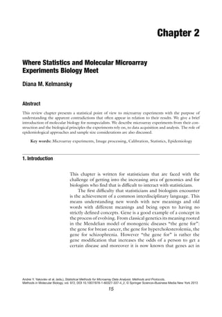
7. 2 Where Statistics and Molecular Microarray Experiments Biology Meet 21
Number of expressed gene copies
30000
10000
0
G1 G20 G41 G62 G83 G106 G131 G156 G181
Gene
Fig. 5. Real hypothetic expression profile.
also segments called introns which are part of the transcribed
mRNA that does not leave the nucleus. This RNA modification in
which introns are removed and exons are joined is called splicing.
The messenger RNA that leaves the nucleus only has exons
and in general is shorter than the original DNA template segment;
it is the mature mRNA that has suffered the capping (G), polyade-
nylation (AAAA…) and splicing processes.
Alternative splicing is the RNA splicing variation mechanism
in which the exons of the primary gene transcript, the pre-mRNA,
are separated and reconnected to produce alternative ribonucle-
otide arrangements. Alternative splicing allows the synthesis of a
greater variety of proteins than the originally DNA segments
expressed have (2).
We will not describe the translation process that directs the
mRNA; however, it is important to keep in mind that the amount
synthesized is relatively proportional to the amount of mRNA
transcribed. It is that amount of mRNA transcribed what we call
gene expression level.
2.5.2. Gene Expression If we could count the number of mRNA molecules for each gene
Profile in a single cell we would obtain its “real expression profile.”
Figure 5 shows a “real hypothetic expression profile.”
3. Microarray
Technologies and
Basic Principles
They Rely On In a microarray experiment the natural process determined by the
central dogma of molecular biology is interrupted to extract mature
mRNA from one or more tissues or cell lines to hybridize it (we’ll
soon see what this is) to its complementary cDNA previously fixed
8. 22 D.M. Kelmansky
on the microarray. The microarray works as a detector of the amount
and kind of mRNA present in the interrogated sample tissue.
Double stranded DNA
↓ transcription or expression
Simple mRNA strand -> cDNA
↓
Microarray
↓ translation
Proteín
3.1. What Are DNA DNA microarrays are small (2.5 cm × 6. 2.5 cm for spotted microar-
Microarrays? rays and 1.28 cm × 1.28 cm for high-density chips), solid supports
onto which the thousands (10,000–1,000,000) of different DNA
sequences are immobilized, or attached, at two dimensional fixed
matrix locations called spots or features. Each spot contains mil-
lions of “identical” sequences.
● Each spot representing a different sequence has a unique phys-
ical location.
● May or may not have knowledge of the sequence.
The supports can be usual glass microscope slides, silicon chips,
or nylon membranes.
According to different array manufacturing technologies
(platforms),
● DNA is printed, spotted, or actually synthesized directly onto
the support.
● Features or spots can either be approximately circles or
rectangles.
● Fixed sequences—DNA, cDNA, short or long DNA oligonu-
cleotides—are called probes.
● Microarrays allow one-color (channel) or two-color experiments.
3.2. Types of Microarrays can be classified according to the kind of the immobi-
Microarrays lized genomic sequences (probes). This is important as the probe
sequences in the array identify complimentary sequences in the
unknown sample genomic sequences (targets).
9. 2 Where Statistics and Molecular Microarray Experiments Biology Meet 23
3.2.1. Transcriptomic The DNA immobilized to the array are complementary DNA
Microarrays sequences (cDNA) derived from known transcribed mRNA
sequences or possible transcribed sequences (putative genes) for a
certain type of tissue, with the purpose of measuring the amount of
copies of the genes that are transcribed in a moment in the experi-
mental tissue. These are called gene expression microarrays.
3.2.2. Comparative
In Comparative Genomic Hybridization (CGH) arrays each spot
Genomic Hybridization
contains DNA cloned sequences with known chromosomal loca-
Array
tion. This allows detecting gains and losses in chromosomes.
Usually probes that map to evenly spaced loci along the entire
length of the genome are printed. Also large pieces of genomic
DNA can serve as the probed DNA.
3.2.3. Polymorphism To detect mutations, immobilized DNA is usually from polymor-
Analysis Array phic variants of a single gene. The probed sequence placed on any
given spot within the array will differ from that of other spots in
the same microarray, sometimes by only one (Single Nucleotide
Polymorphism, or SNP) or a few specific nucleotides.
3.3. Basic Principles DNA microarrays rely on the complementary rule: under adequate
on Which Microarray experimental conditions, complementary single stranded nucleic
Experiments Rely On have strong tendency of binding in a double stranded nucleic acid
molecule.
For every mRNA sequence of interest (target) a complemen-
tary DNA sequence (cDNA) can be obtained to immobilize a probe
for that sequence onto the solid support. The position of the probe
in the array identifies the sequence.
3.3.1. Nucleic Acid The chemical process by which two complementary single stranded
Hybridization nucleic acid chains zipper up to form a double stranded molecule
and Denaturation is called hybridization.
When double stranded DNA molecules are subjected to condi-
tions (pH, temperature, etc.) that disrupt their hydrogen bonds,
the strands are no longer held together. This means that the strands
separate as individual coils, it is then said that the double helix is
denatured.
The denaturation conditions differ according to the relative
G + C content in the DNA. The higher the G + C content of a
DNA, the higher its denaturation temperature because G–C pairs
are held by three H bonds whereas A–T pairs have only two.
The DNA denaturation is reversible. This process is called
DNA renaturation or hybridization.
Hybridization reactions can occur between any (even those
coming from different species) complementary single stranded
nucleic acid chains: DNA/DNA, RNA/RNA, DNA/RNA.
Both denaturation and hybridization processes are important
in microarray experiments.
10. 24 D.M. Kelmansky
3.4. Sample Genetic As we have already seen, the normal cellular modification of mRNA
Material includes the polyadenylation process, this is the addition of up to
200 adenine nucleotides to one end of the molecule called poly(A)
3.4.1. mRNA Isolation
tail. In order to isolate mRNA from a given tissue, its cells are bro-
ken up and the cellular contents are exposed to beads coated with
strings of thymine nucleotides. Because of adenine and thymine
binding affinity the poly(A) mRNA is selectively retained on the
beads while the other cellular components are washed away.
3.4.2. Reverse Once isolated, purified mRNA is converted to single stranded
Transcription DNA using the enzyme reverse transcriptase and is then made into
a stable double stranded DNA using the enzyme DNA polymerase.
DNA produced in this way is called complementary DNA (cDNA)
because its sequence, at least the first strand, is complementary to
that of the mRNA from which it was made, and represents only
exon DNA sequences.
4. Microarray
Experiments.
General
and Specific In gene expression microarrays experiments the amount of mRNA
Remarks (in a given tissue at a given moment for each sequence probed in
the array) is measured indirectly using dye labelled molecules in
order to answer, for example:
● How gene expression differs in different cell types.
● How gene expression differs in a normal and diseased (e.g.,
cancerous) cell.
● How gene expression changes when a cell is treated by a drug.
● How gene expression changes when the organism develops
and cells are differentiating.
● How gene expression is regulated—which genes regulate
which and how.
There are six general steps to follow in the microarray
experiments:
● Relevant questions, statistical experiment design.
● Microarray manufacturing.
● Sample preparation and target labelling.
● Hybridization of the labelled target samples sequences to the
corresponding microarray probes.
● Washing to eliminate the excess solution and reduce the
nonspecific binding.
● Scanning the microarray under laser light and obtaining a digi-
tal image.
11. 2 Where Statistics and Molecular Microarray Experiments Biology Meet 25
The initial data resulting from microarray experiments are one
or two digital images, depending on the microarray platform used,
for every microarray. Three more data analysis steps follow:
● Image analysis.
● Calibration.
● Statistical data analysis.
4.1. Design Many experimental researchers, believe that statistical issues can be
of secondary importance at the early stages of the experiment and
that statisticians should be incorporated at the data analysis and
interpretation phase of the investigation. However, also in this
research area, data analysis cannot compensate for inadequate
design. For microarrays experiments it is important to remember
that different experimental conditions may give different expres-
sion profiles for the same biological setting (3).
The proposals for experimental design- and model-based anal-
ysis taking into account random variability are not new (4–6). We
will only describe a few specific aspects regarding the array design
and the samples design.
4.1.1. Array Design The choice of the DNA probe sequences to be synthesised or spot-
ted on to the array depends on the technology and the type of
genes the researcher wishes to interrogate or by the cDNA libraries
(collections of cDNA clones) available. For high-density in situ
synthesized short oligos (25 bases) microarrays it is mainly the
manufactures’ decision; however, specific custom arrays can also be
ordered at higher costs. Many researchers also buy or make their
own spotted cDNA or long oligos (60–70 bases) microarrays. In
the design of these arrays they must decide:
● Which and where the probes will be spotted.
● Which and where the controls will be spotted.
Controls are special probes included in the array, some have the
purpose of evaluating the quality of the experiment and others will be
used to standardise the measurements. The usual control probes are:
● Negative controls: Empty spots, buffer solution spots.
● Level controls: Spots with cDNA or oligos from different spe-
cies that will not interfere with the sampled genomic sequences
(i.e., bacterial DNA if mammals are studied) complementary
sequences will be added to the samples (spiked in) in pre
specified quantities. Their intensity values serve for
calibration.
● Positive controls: “Housekeeping genes,” highly expressed
genes in all samples to evaluate if the hybridization has effec-
tively occurred.
12. 26 D.M. Kelmansky
Adjacent duplicate spots (two or more times) are included to
evaluate signal variation. However this estimation will be lower
than the real meaningful between array variability for a given spot
among replicated arrays.
4.1.2. Sample Design When multiple microarrays are hybridized with mRNA from a sin-
gle biological case we have technical replicates. These replications
Technical Replicates
only allow measuring the variability due to measurement errors
and are useful in quality-control studies.
Biological Replicates Biological replicates allow the evaluation of both measurement
variability and biological differences between cases. This type of
replication is obtained when the sample mRNA comes from differ-
ent individuals from a given species or different cell lines and is
required when the aim is to make inferences about populations.
Although early microarray experiments used few or no biological
replicates, their necessity is now undisputed (7).
Sample Size Early microarray studies (8–10) used a single “two channel”
microarray or two “one channel” microarrays to identify differen-
tially expressed genes. Several proposals were developed to deal
with the problem (11–13). The idea behind the proposals was that
the measurements on many genes, i.e., variables, could compen-
sate the reduced sample size. Sizes of 2 or 3 were considered large.
This point of view is changing to realize that even if technical vari-
ability was eliminated it is not possible to reduce random variability
inherent to biological processes and that there is no alternative to
increasing samples sizes in microarray studies (14).
Observational Studies In many microarray experiments sample DNA or RNA come from
observational studies. Bias and confounding factors should have
been considered as they are in any epidemiological study; however
this has not been the practise in such experiments (15, 16) which
in general lack of standard epidemiological approaches (i.e., assess-
ment of chance, bias, and confounding). The advantages that
microarray technology can introduce in clinical and epidemiologi-
cal studies, if well established epidemiologic principles are not
sacrificed in the process, is beginning to be noticed (17).
5. Image Analysis
The resulting data from a microarray experiment are one or two
digital images for each microarray in the experiment. These
microarray digital images (18) provide a snapshot of the types and
quantities of molecules that have reacted during hybridization and
hence were present in the sample targets.
13. 2 Where Statistics and Molecular Microarray Experiments Biology Meet 27
A microarray image is a two-dimensional numeric representa-
tion in which each value gives the mean intensity of a small sector
or pixel. Every spot is represented by hundreds of pixels and we
have pixel wise data. It is necessary to obtain a summary intensity
measure for each spot in the array.
Image processing can be divided in three tasks
● Gridding: It is the assignment of spots’ coordinates.
● Segmentation: Classification of foreground (signal) and back-
ground pixels.
● Target intensity extraction: Obtaining a summary measure of
the spot intensity from the foreground and background pixels.
Perhaps the most critical aspect of image processing is segmen-
tation; this is deciding which pixels correspond to the signal for
each spot. There are four commonly used segmentation methods:
fixed circle, variable circle, histogram, and adaptive shape. It has
not yet been established and it is not clear if there exists an optimal
method (19–23). High-density oligonucleotide spots are square,
and squared regions are considered for the spot foreground and
background summary measures (24).
Standard image processing methods subtract background from
foreground intensities to obtain the final intensity value for each
pixel. This background correction gives negative signals for microar-
ray images. Several proposals (19–22) deal with this drawback, as
missing values are artificially generated with the usual base 2 loga-
rithmic (log2) data transformation used. Image analysis including
background correction methods still is an active research area.
Probe wise data are the final result of the image processing stage.
These are the data we are considering in subsequent sections.
Data from high-density microarrays require a preliminary sum-
marizing step, that of probe intensities that interrogate the same
genomic sequence (25, 26).
6. Data Calibration
Data from microarray experiments show two types of problems
that are faced through data transformations:
1. MA plots present curved structures not attributable to biologi-
cal reasons.
2. Probe intensity variability is mean dependent.
Let Yrk represent the intensity of probe k in array r that resulted
from the image processing stage. MA plots compare the intensity
of two “one channel” arrays (or the two channels of a two channel
microarray) in scatter plots of
14. 28 D.M. Kelmansky
Mk = log2 (Y1k/Y2k) in the y-axes.
Ak = 0.5 log2 (Y1k × Y2k) in the x-axes.
If the samples of both arrays (or channels of the same array)
come from identical biological conditions (self–self experiment) no
tendency is expected in a MA plot. However curved structures not
attributable to biological reasons are usually seen in these plots.
A very frequently used procedure that eliminates such struc-
tures consists in subtracting, to every M value in the plot, the fit of
a local smoother in the original MA plot. The data on that curve
are representing the probes with no different expression between
the compared arrays (27). The transformed data can be written as
Ck
Z rk = log 2 (Yrk ) + , (1)
2
where C k is a constant depending on the spot and the local
smoother. This procedure is straight forward and flexible enough
to capture most of the structures appearing in MA plots but we are
forcing the data to satisfy our expectations.
The data transformation given in Eq. 1 solves the first of the
two problems stated at the beginning of this section and partially
the second one.
In relation to the mean variance dependence of microarray
intensity data several authors coincide in modelling intensities
through a multiplicative additive model (28, 29)
Yrk = ar + br X rk e ηk +ςrk + εk + δrk , (2)
where Xrk is the true intensity of spot k in array r; ar , br are con-
stants and ηk , ς rk , εk , δrk are error terms. Moreover the following
transformation
Z rk = log(Br Yrk + Cr + (Br Yrk + Cr )2 + 1),
has independently been proposed by several authors (30–32) to
stabilize the variance in microarray data that satisfy the multiplica-
tive additive model (2) and the array dependent constants Br , Cr
are estimated from the data. This transformation is based on a qua-
dratic relationship between the variance and signal strength in the
original scale if the data meet the model (2). This model can also
explain all structures that are found in MA plots (33). Even if only
the nonrandom components are considered, the nonlinear depen-
dencies can be explained and removed, giving a much simpler
interpretation: the true intensities are related to the observed
intensities through an affine transformation
Y = a + b ·X .
and different choices for the parameters of the affine transformation
for different arrays give the patterns observed in MA plots (34).
15. 2 Where Statistics and Molecular Microarray Experiments Biology Meet 29
7. Statistical
Analysis
7.1. Inference One of the basic statistical inference concerns is to conduct tests to
decide whether the difference of two sample means provides enough
evidence to decide that the population means are different. In a
microarray context it comes to detect genes with mean different
expression levels between two or more groups (types of tissue) that
provide enough evidence to decide that the genes are differentially
expressed. The problem arises from the fact that thousands of tests
must be conducted, one for each genomic sequence of interest.
There is a widespread agreement that multiple comparison
procedures should be used. The usually recommended procedure
is the false discovery rate (FDR). The argument in favour of using
this error rate is based on the fact that the usual correction which
is obtained by using the classical Bonferroni procedure is too
restrictive resulting in a reduction in power. However the strong
coregulation gene structures lead to very unstable estimation of
the FDR. A Bonferroni type procedure controlling the expected
value of false positives results in more stable estimates than those
from FDR in comparable powers (35).
Multiple comparisons can be reduced and power improved
through the comparison of a priori defined subsets of genes; the
subsets are tested between two biological states in what is called
“gene subset enrichment analysis (GSEA)” (36). This 2003 pro-
posal, that uses groups of genes that share common biological
function, chromosomal location, or regulation, has been used in a
number of applications (37–39) and is going through subsequent
improvements (40–47).
7.2. Classification Unsupervised classification is one of the first statistical techniques
used in the analysis of microarray data and is one of the favourites.
This method attempts to divide the data into classes without prior
information (unsupervised classification) or predefined classes. It
has shown some successes in finding relevant and meaningful pat-
terns (48–51). However, the researcher is guaranteed to obtain
gene clusters, regardless of
● Sample size.
● Data quality.
● The design of the experiment.
● Any other biological validity that is affiliated with the
grouping.
Unsupervised classification should be avoided, if it is inevitable,
some sort of reproducibility measure should be provided. Those
procedures that re-sample at case level—rather than gene level—
have a reasonable performance and none is considered the best.
16. 30 D.M. Kelmansky
Supervised classification procedures need an independent cross
validation as the resulting prediction rules are based on a relatively
small number of samples of various types of tissues containing
expression data of many thousands of genes.
The results of classification procedures may be representing to
the data too much giving low or null predictive power; this is what
is called over fitting.
8. Challenges
Microarray technologies generated explosive expectations related to
the advances that in biology and medicine would occur in the short
term (51, 52) but as results did not parallel those expectations the
literature reflected the disappointments (53). As the technology of
microarrays ran ahead of analysis techniques, researchers from vari-
ous fields carried out their own statistics to analyze the data (54).
A growing number of publications per year from the year 1995
appeared since Schena (55) presented his first work on such experi-
ments. Figure 6 shows the number of microarrays publications per
year (selecting in Pub Med for the keywords “microarray or
microarrays”). The number of articles per year has an exponential
growth from 1995 to 2001. From then until 2005 the growth is
linear with about a thousand more publications every year. The
value of 2006 deviates slightly below this trend and in 2007 the
deviation is even further.
8.1. Some Successes In the decade since the beginning of technology, there have also
been successes. Patients with leukaemia were automatically and
accurately classified in two main subtypes of the disease using only
Number of publications from PubMed
6000
4000
2000
0
1996 1998 2000 2002 2004 2006
Year
Fig. 6. Number of publications selected with “microarray or microarrays” keywords.
17. 2 Where Statistics and Molecular Microarray Experiments Biology Meet 31
gene expression levels in 1999 (56). While these forms of leukaemia
were already known and well characterized, the experiment showed
that the strategy could in principle reveal unknown subtypes.
Further in 2001, researchers identified five patterns of gene expres-
sion levels in breast cancer (57) and showed that corresponded to
different types of diseases with different prognosis.
More recently in 2006 a gene with a fold-change of 50 times
the level of expression in cancer patients who did not respond to
chemotherapy treatment in comparison to those who did respond
to treatment was found (58). This gene encodes for a protein that
prevents tumour cell death; blocking this protein might allow a
chemotherapy response.
In 2005, the US Food and Drug Administration (FDA) approved
the first microarray-based clinical test. The test identifies genetic
variations in two key codifying regions CYP2D6 and CYP2C19 for
the cytochrome P450 enzyme that metabolizes usual drugs. This
will enable doctors to personalize drug choice and dosing (59).
8.2. Frustrations Also, in the decade since the advent of microarray technology a
great deal of frustration has accumulated among biologists who
have dedicated their efforts in following up false research direc-
tions. Many articles have been discredited; scientists have difficulties
in finding studies that point to something concrete and in validat-
ing the results and several articles show this frustration (60–62).
Several studies (63–65) have found that the list of differentially
expressed genes has had very low overlap between different plat-
forms. However the overlap among independent studies for the
same biological question can have important improvements if
coherent statistical analysis are carried out (66).
Numerous discussions in the literature show a tendency to
explain the glaring lack of power and instability of the results of
data analysis, by a high technical level of noise in the data.
The Quality Control (MAQC) Consortium project has generated
public available databases that may give an answer to the referred dis-
cussions (67). These technical replicates addresses the evaluation of
● Repeatability within a single site.
● Reproducibility between sites.
● Comparability between platforms.
Several papers reporting the analysis of MACQ data (68–73)
are showing promising results on the reliability and reproducibility
of microarray technology and reflecting that the random fluctuations
of gene expression signals caused by technical noise are quite low.
So, how are problems explained? Fig. 7 shows the number of
publications selected with “microarray or microarrays” and “statis-
tics or statistical” keywords. Its striking the low number of microar-
ray publications presenting statistical analysis.
18. 32 D.M. Kelmansky
Number of publications from PubMed
6000
microarrays
statistics and microarrays
4000
2000
0
1996 1998 2000 2002 2004 2006
Year
Fig. 7. Number of publications selected with “microarray or microarrays” and “statistics or statistical” keywords.
9. Conclusions
Microarray experiments present two main types of difficulties. The
first one is microarray reliability. The MACQ project currently
addresses the evaluation of the repeatability within a single site,
between sites reproducibility and comparability between platforms.
Although some researchers believe that experiments addressed in
the MAQC project are conducted in conditions too “ideal” and
that hardly reflect the real situation of many experimental labora-
tories (74) and sample sizes are not large enough (75), in general
the results are satisfactory (76). Moreover, this technology is con-
stantly evolving and improving, so it is expected to provide better
and lower budget results.
The second difficulty lies in the design of the experiment and
data analysis. It is important to incorporate epidemiological prin-
ciples to the experiment design whenever dealing with observa-
tional studies. Also, microarray research area would benefit from
identical design and statistical analysis for different experiments on
a given biological problem. The second aspect of this goal would
be achieved if researchers made available their raw data for reanaly-
sis. Even better would be if research on one topic conducted by
independent labs would follow the same protocol. This, together
with the reduction of the experimental costs, may increase sample
sizes and thus an improve power. A deeper understanding of nor-
mal biological variability and gene coregulation mechanisms could
be addressed (77, 78). It is critical to the advancement of knowl-
edge in molecular biology that microarrays no longer be simply
used as exploratory tools.
19. 2 Where Statistics and Molecular Microarray Experiments Biology Meet 33
References
1. http://www-lbit.iro.umontreal.ca/ISMB98/ using appropriate designs. Trends Genet
anglais/ontology.html 19(12):690–695
2. Lopez AJ (1998) Alternative splicing of 17. Webb PM, Melissa A, Merritt MA, Boyle MG,
pre-mRNA: developmental consequences and Green AC (2007) Microarrays and epidemiol-
mechanisms of regulation. Annu Rev Genet ogy: not the beginning of the end but the end
32:279–305 of the beginning. Cancer Epidemiol Biomarkers
3. http://www.affymetrix.com/support/techni- Prev 16:637–638
cal/technotes/blood_technote.pdf 18. Schena M (2003) Microarray analysis. Wiley-
4. Churchill GA (2002) Fundamentals of experi- Liss, Hoboken, NJ. ISBN 9780471414438
mental design for cDNA microarrays. Nat 19. Yang YH, Buckley MJ, Speed TP (2001)
Genet 32:490–495 Analysis of cDNA microarray images.
5. Kerr MK, Churchill GA (2001) Statistical Bioinformatics 2(4):341–349
design and the analysis of gene expression 20. Yang YH, Dudoit S, Luu P, Lin DM, Peng V,
microarray data. Genet Res 77(2):123–128 Ngai J, Speed TP (2002) Normalization for
6. Smyth GK, Yang YH, Speed T (2003) Statistical cDNA microarray data: a robust composite
issues in cDNA microarray data analysis. method addressing single and multiple slide
Methods Mol Biol 224:111–136 systematic variation. Nucleic Acids Res 30:e15
7. Allison D, Cui X, Page G, Sabripour M (2006) 21. Angulo J, Serra J (2003) Automatic analysis of
Microarray data analysis: from disarray to DNA microarray images using mathematical
consolidation and consensus. Nat Rev Genet morphology. Bioinformatics 19(5):553–562
7:55–65 22. Li Q, Fraley C, Bumgarner R, Yeung K, Raftery
8. DeRisi J, Penland L, Brown PO, Bittner ML, A (2005) Donuts, scratches and blanks: robust
Meltzer PS, Ray M, Chen Y, Yan AS, Trent JM model-based segmentation of microarray
(1996) Use of a cDNA microarray to analyse images. Technical Report no. 473. Department
gene expression patterns in human cancer. Nat of Statistics, University of Washington
Genet 14:457–460 23. Ahmed A, Vias M, Iyer N, Caldas C, Brenton
9. Schena M, Shalon D, Davis RW, Brown PO J (2004) Microarray segmentation methods
(1995) Quantitative monitoring of gene significantly influence data precision. Nucleic
expression patterns with a complementary Acids Res 32(5):1–7
DNA microarray. Science 270:467–470 24. Wu Z, Irizarry R, Gentleman R, Murillo F,
10. Schena M (1996) Genome analysis with gene Spencer F (2003) A model based background
expression microarrays. BioEssays 18:427–431 adjustment for oligonucleotide expression
11. Chen Y, Dougherty E, Bittner M (1997) arrays CGRMA-MLE. Technical Report, John
Ratio-based decisions and the quantitative Hopkins University, Department of
analysis of cDNA microarray images. J Biomed Biostatistics, Baltimore, MD. Working Papers
Opt 2(4):364–374 25. Irizarry R, Hobbs F, Beaxer-Barclay Y,
12. Newton M, Kendziorskim M, Richmond C, Antonellis K, Scherf U, Speed T (2003)
Blattner F, Tsui K (2001) On differential vari- Exploration, normalization, and summaries of
ability of expression ratios: improving statistical high density oligonucleotide array probe level
inference about gene expression changes from data. Biostatistics 4:249–264
microarray data. J Comput Biol 8(1):37–52 26. Irizarry RA, Bolstad BM, Collin F, Cope LM,
13. Sapir M, Churchill GA (2000) Estimating the Hobbs B, Speed TP (2003) Summaries of
posterior probability of differential Affymetrix GeneChip probe level data. Nucleic
gene,expression from microarray data. Poster, Acids Res 31(4):e15
The Jackson Laboratory. http://www.jax. 27. Yang YH, Dudoit S, Luu P, Lin DM, Peng V,
org/research/churchill/pubs/marina.pdf Ngai J, Speed TP (2002) Normalization for
14. Klebanov L, Yakovlev A (2007) Is there an alter- cDNA microarray data: a robust composite
native to increasing the sample size in microarray method addressing single and multiple slide
studies? Bioinformation 1(10):429–431 systematic variation. Nucleic Acids Res
15. Potter JD (2001) At the interfaces of epidemi- 30:e15
ology, genetics, and genomics. Nat Rev Genet 28. Durbin BP, Hardin JS, Hawkins DM, Rocke
2:142–147 DM (2002) A variance estabilizing transfor-
16. Potter JD (2003) Epidemiology, cancer genet- mation for gene expression microarray data.
ics and microarrays: making correct inferences, Bioinformatics 18:105–110
20. 34 D.M. Kelmansky
29. Huber W, Von Heydebreck A, Sultmann H, Inactivation of the Snf5 tumor suppressor stim-
Poustka A, Vingron M (2002) Variance stabili- ulates cell cycle progression and cooperates with
zation applied to microarray data calibration p53 loss in oncogenic transformation. Proc Nat
and to the quantification of differential expres- Acad Sci U S A 102(49):17745–17750
sion. Bioinformatics 18:96–104 40. Xiao Y, Frisina R, Gordon A, Klebanov LB,
30. Munson P (2001) A “consistency” test Yakovlev AY (2004) Multivariate search for
for determining the significance of gene differentially expressed gene combinations.
expression changes on replicate samples and BMC Bioinform 5(1):164
two-convenient variance-stabilizing trans- 41. Dettling M, Gabrielson E, Parmigiani G
formations. GeneLogic Workshop on Low (2005) Searching for differentially expressed
Level Analysis of Affymetrix GeneChip Data, gene combinations. Genome Biol 6:R88
Nov. 19, Bethesda, MD 42. Subramanian A, Tamayo P, Mootha VK,
31. Durbin BP, Hardin JS, Hawkins DM, Rocke Mukherjee S, Ebert BL, Gillette MA, Paulovich
DM (2002) A variance estabilizing transfor- A, Pomeroy SL, Golub TR, Lander ES,
mation for gene expression microarray data. Mesirov JP (2005) Gene set enrichment analy-
Bioinformatics 18:105–110 sis: a knowledge-based approach for interpret-
32. Huber W, von Heydebreck A, Sueltmann H, ing genome-wide expression profiles. Proc
Poustka A, Vingron M (2003) Parameter estima- Natl Acad Sci U S A 102(43):15545–15550
tion for the calibration and variance stabilization 43. Tian L, Greenberg SA, Kong SW, Altschuler J,
of microarray data. Stat Appl Genet Mol Biol Kohane IS, Park PJ (2005) Discovering statis-
2:3.1–3.22 tically significant pathways in expression
33. Cui X, Kerr M, Churchill G (2003) profiling studies. Proc Natl Acad Sci U S A
Transformations for cDNA microarray data. 102(38):13544–13549
Stat Appl Genet Mol Biol 2(1) Article 4 44. Barry WT, Nobel AB, Wright FA (2005)
34. Bengtsson H, Hössjer O (2006) Methodological Significance analysis of functional categories in
study of affine transformations of gene expres- gene expression studies: a structured permuta-
sion data with proposed robust non-parametric tion approach. Bioinformatics 1(9):1943–1949
multi-dimensional normalization method. 45. Efron B, Tibshirani R (2007) On testing the
BMC Bioinform 7(100):1–18 significance of sets of genes. Ann Appl Stat
35. Gordon A, Glazko G, Qiu X, Yakovlev A 1(1):107–129
(2007) Control of the mean number of false 46. Klebanov L, Glazko G, Salzman P, Yakovlev A
discoveries, Bonferroni and stability of multiple (2007) A multivariate extension of the gene
testing. Ann Appl Stat 1(1):179–190 set enrichment analysis. J Bioinform Comput
36. Mootha VK, Lindgren CM, Eriksson KF, Biol 5(5):1139–1153
Subramanian A, Sihag S, Lehar J, Puigserver P, 47. Eisen MB, Spellman PT, Brown PO, Botstein
Carlsson E, Ridderstrale M, Laurila E, Houstis D (1998) Cluster analysis and display of
N, Daly MJ, Patterson N, Mesirov JP, Golub genomewide expression patterns. Proc Natl
TR, Tamayo P, Spiegelman BM, Lander ES, Acad Sci U S A 95(25):14863–14868
Hirschhorn JN, Altshuler D, Groop LC (2003) 48. Golub TR, Slonim DK, Tamayo P, Huard C,
PGC-1alpha-responsive genes involved in Gassenbeek M, Mesirov JP, Coller H, Loh
oxidative phosphorylation are coordinately ML, Downing JR, Caligiuri MA, Bloomfield
downregulated in human diabetes. Nat Genet DD, Lander ES (1999) Molecular classification
34:267–273 of cancer: class discovery and class prediction
37. Lamb J, Ramaswamy S, Ford HL, Contreras by gene expression monitoring. Science
B, Martinez RV, Kittrell FS, Zahnow CA, 286(15):531–537
Patterson N, Golub TR, Ewen ME (2003) A 49. Tamayo P, Slonim D, Mesirov J, Zhu Q,
mechanism of cyclin D1 action encoded in the Kitareewan S, Dmitrovsky E, Lander ES
patterns of gene expression in human cancer. (1999) Interpreting patterns of gene expres-
Cell 114(3):323–334 sion with self-organizing maps: methods and
38. Majumder PK, Febbo PG, Bikoff R, Berger R, application to hematopoietic differentiation.
Xue Q, McMahon LM, Manola J, Brugarolas J, Proc Natl Acad Sci U S A 96(6):2907–2912
McDonnell TJ, Golub TR, Loda M, Lane HA, 50. Wen X, Fuhrman S, Michaelis GS, Carri DB,
Sellers WR (2004) mTOR inhibition reverses Smith S, Barker SJ, Somogyi R (1998) Large-
Akt-dependent prostate intraepithelial neoplasia scale temporal gene expression mapping of
through regulation of apoptotic and HIF-1- central nervous system development. Proc
dependent pathways. Nat Med 10(6):594–601 Natl Acad Sci U S A 95:334–339
39. Isakoff MS, Sansam CG, Tamayo P, Subramanian 51. Lander E (1999) Array of hope. Nat Genet
A, Evans JA, Fillmore CM, Wang X, Biegel JA, (Supplement 21)
Pomeroy SL, Mesirov JP, Roberts CW (2005)
21. 2 Where Statistics and Molecular Microarray Experiments Biology Meet 35
52. Schena M (2003) Microarray analysis preface 66. Suárez-Fariñas M, Noggle S, Heke M,
page XIV. Wiley-Liss, Hoboken, NJ. ISBN Hemmati-Brivanlou, Magnasco M (2005)
9780471414438 Comparing independent microarray studies:
53. Frantz S (2005) An array of problems. Nat Rev the case of human embryonic stem cells. BMC
Drug Discov 4:362–363 Genomics 6(99):1–11
54. Cobb K (2006) Re inventing statistics in 67. MAQC Consortium (2006) The MicroArray
microarrays: the search for meaning in a vast Quality Control (MAQC) project shows inter-
sea of data. Biomed Comput Rev 2(4):21 and intraplatform reproducibility of gene
55. Schena M, Shalon D, Davis RW, Brown PO expression measurements. Nat Biotechnol
(1995) Quantitative monitoring of gene 24(9):1151–1161
expression patterns with a complementary 68. Bosotti R et al (2007) Cross platform micro-
DNA microarray. Science 270:467–470 array analysis for robust identification of
56. Golub TR, Slonim DK, Tamayo P, Huard C, differentially expressed genes. BMC Bioinform
Caasenbeek M, Mesirov JP, Coller H, Loh ML, 8(Suppl 1):S5
Downing JR, Caligiuri MA, Bloomfield CD, 69. Wang Y et al (2006) Large scale real-time PCR
Lander ES (1999) Molecular classification of can- validation on gene expression measurements
cer: class discovery and class prediction by gene from two commercial long-oligonucleotide
expression monitoring. Science 286:531–537 microarrays. BMC Genomics 7:59
57. Sorlie et al (2001) Gene expression patterns of 70. Kuo WP et al (2006) A sequence-oriented
breast carcinomas distinguish tumor subclass comparison of gene expression measurements
with clinical implications. Proc Natl Acad Sci across different hybridization-based technolo-
USA 98(19):10869–10874 gies. Nat Biotechnol 24(7):832
58. Petty RD, Kerr KM, Murray GI, Nicolson 71. Canales RD et al (2007) Evaluation of DNA
MC, Rooney PH, Bissett D, Collie-Duguid ES microarray results with quantitative gene
(2006) Tumour transcriptome reveals the pre- expression platforms. Nat Biotechnol 24(9):
dictive and prognostic impact of lysosomal 1115
protease inhibitors in non-small-cell lung can- 72. Klebanov L, Yakovlev A (2007) How high is
cer. J Clin Oncol 24(11):1729–1744 the level of technical noise in microarray data?
59. http://www.medicalnewstoday.com/arti- Biol Direct 2:9
cles/18822.php 73. Robinson MD, Speed TP (2007) A compari-
60. Frantz S (2005) An array of problems. Nat Rev son of Affymetrix gene expression arrays. BMC
Drug Discov 4:362–363 Bioinform 15(8):449
61. Ioannidis JPA (2005) Microarrays and molec- 74. Perkel J (2006) Six things you won’t find in
ular research: noise discovery? The Lancet the MAQC. Scientist 20(11):68
365(9458):454–455 75. Klebanov L, Qiu X, Welle S, Yakovlev A (2007)
62. Marshall E (2004) Getting the noise out of Statistical methods and microarray data. Nat
gene arrays. Science 306:630–631 Biotechnol 25:25–26
63. Tan PK et al (2003) Evaluation of gene expres- 76. http://www.microarrays.ca/MAQC_Review_
sion measurements from commercial microarray July2007.pdf
platforms. Nucleic Acids Res 31:5676–5684 77. Klebanov L, Jordan C, Yakovlev A (2006) A
64. Miller RM et al (2004) Dysregulation of gene new type of stochastic dependence revealed in
expression in the 1-methyl-4-phenyl-1,2,3,6- gene expression data. Stat Appl Genet Mol
tetrahydropyridine-lesioned mouse substantia Biol 5:1
nigra. J Neurosci 24(34):7445 78. Klebanov L, Yakovlev A (2007) Diverse cor-
65. Miklos GL, Maleszka R (2004) Microarray relation structures in gene expression data and
reality checks in the context of a complex dis- their utility in improving statistical inference.
ease. Nat Biotechnol 22:615–621 Ann Appl Stat 1(2):538–559