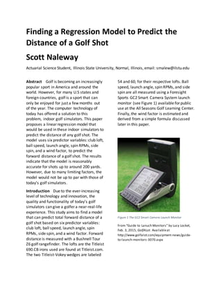
1. Finding a Regression Model to Predict the
Distance of a Golf Shot
Scott Naleway
Actuarial Science Student, Illinois State University, Normal, Illinois, email: srnalew@ilstu.edu
Abstract Golf is becoming an increasingly
popular sport in America and around the
world. However, for many U.S states and
foreign countries, golf is a sport that can
only be enjoyed for just a few months out
of the year. The computer technology of
today has offered a solution to this
problem, indoor golf simulators. This paper
proposes a linear regression model that
would be used in these indoor simulators to
predict the distance of any golf shot. The
model uses six predictor variables: club loft,
ball speed, launch angle, spin RPMs, side
spin, and a wind factor, to predict the
forward distance of a golf shot. The results
indicate that the model is reasonably
accurate for shots up to around 200 yards.
However, due to many limiting factors, the
model would not be up to par with those of
today’s golf simulators.
Introduction Due to the ever-increasing
level of technology and innovation, the
quality and functionality of today’s golf
simulators can give a golfer a near-real-life
experience. This study aims to find a model
that can predict total forward distance of a
golf shot based on six predictor variables:
club loft, ball speed, launch angle, spin
RPMs, side spin, and a wind factor. Forward
distance is measured with a Bushnell Tour
Z6 golf rangefinder. The lofts are the Titleist
690.CB irons used are found at Titleist.com.
The two Titleist-Vokey wedges are labeled
54 and 60, for their respective lofts. Ball
speed, launch angle, spin RPMs, and side
spin are all measured using a Foresight
Sports GC2 Smart Camera System launch
monitor (see Figure 1) available for public
use at the All Seasons Golf Learning Center.
Finally, the wind factor is estimated and
derived from a simple formula discussed
later in this paper.
Figure 1 The GC2 Smart Camera Launch Monitor
From “Guide to Lanuch Monitors” by Lucy Locket,
Feb. 3, 2015, GolfALot. Availableat
http://www.golfalot.com/equipment-news/guide-
to-launch-monitors-3070.aspx

2. All of the data on the golf shots is
collected in one day. A Microsoft Excel
spreadsheet is used to record and organize
the data for statistical testing. All of the
statistical testing and the extraction of the
regression model is performed using the
statistical computing software R. The data is
split into two categories: Model-Building
data and a holdout sample used for Model
Validation. Most of the testing and initial
regression model is derived from the
Model-Building data, then tested on the
Model-Validation data for consistency and
prediction ability, and finally the two data
sets are combined and a final model is
produced.
Limitations Due to the limited
availability of resources for an ISU
undergraduate in Bloomington-Normal, the
goal of this study is not to find a model that
will exceed or improve those models used
in today’s golf simulators, but one that will
simply be able to reasonably predict
distance. Limiting factors and restrictions
for this study are as follows:
1. All data is collected on one day. The
temperature does not vary much,
the wind direction does not vary
much, and we are limited to the
amount of balls we can hit because
we are deep into an Illinois winter,
the five-month off-season for Mid-
Western golfers. In other words, my
brother and I are out of shape.
2. The range balls used in the study
were inconsistent. There are three
different types of range balls, some
brand new, some worn and without
dimples. These inconsistencies in
the balls account for a great deal of
error in the data.
3. The distance of each shot is
measured with a Bushnell TourZ6
golf rangefinder. It uses an infrared
laser to measure distance. It is
accurate to within half of one yard
from 5-200 yards. It can give this
accurate reading of distance to an
object, pin, tree wall and even the
ground. However, the response(Y)
variable is total forward distance.
For example, one golfer hits a 200
yard shot at a 30-degree angle to
the right. Another golfer hits a 200
yard shot right down the middle of
the fairway. The first golfer is not as
close to the pin as the second golfer.
This is why forward distance is the
most crucial of the two distances.
The rangefinder can only accurately
measure the distance from tee to
ball; therefore, the total forward
distance needs to be estimated. If a
spotter could be out on the range,
this would remove the need for
estimation. However, due to safety
and liability reasons, the All Seasons
Golf Learning Center does not
permit anyone to walk out onto the
range for any reason.
4. The range itself has an upward slope
with negative convexity and many
small hills and valleys. This causes
two inconveniences. First, due to
the negative convexity of the range,
the accurate measurement of
distance beyond 200 yards becomes
nearly impossible. Due to this
hindrance, the study only includes
shots from the 3-iron to the 60-
degree lob wedge. No woods or
drivers are used. This is a serious
problem because woods are
constructed with different materials
and for different purposes than

3. irons. Generally speaking, the shot
distance between clubs for any
golfer rapidly increases as loft
decreases. The distance between a
9-degree driver and a 13-degree 3-
wood is much greater than the
distance between a 48-degree
pitching wedge and a 44-degree 9-
iron. This missing data from the
study will have a substantial,
negative impact on the overall
usability of the model. Second, any
ball that ends up in a valley behind a
small is no longer visible to the
rangefinder and therefore, its
distance is estimated.
5. Due to the inability to locate an
anemometer, there is no accurate
way to measure wind speed and
direction.
6. Only one set of irons are used in the
study. This could lead to a biased
data set.
7. Only two golfers are used in the data
collection. This could lead to a
biased data set.
Data Collection All of the data from 100
shots is recorded. Since all of the data has
to collected in one day, data from the first
70 shots is used for the model-building data
set and a holdout is saved for model
validation. The initial plan was to hit 120
shots and have the model-building data set
and the validation data set be an equal 60
each, however due to encroaching fatigue
and soreness from hitting 100 golf balls for
the first time in months forced us to adjust
the experiment. In addition to 100 golf
shots, a gentleman from the pro shop hit
five shots and I hit four more shots to be
used for prediction intervals after the full
and final model is acquired.
On the day of the data collection,
the weather was brisk. It was about 50
degrees and the wind averaged about 15
MPH WNW, according to the Weather
Channel App. The driving range faces due
North, so from a golfer’s standpoint, the
wind was blowing to the right and “a bit in
our faces.” The wind remained fairly
consistent with some gusts here and there
and for about the last 15 shots or so, the
wind speed decreased substantially. The
process of hitting golf balls, measuring and
collecting data would take three hours to
complete. In order to conserve energy,
Mark and I would take turns, hitting every
other six shots. I always measure the
distance to the ball for consistency. Data
from the rangefinder, launch monitor and
wind estimation is collected for every shot.
A total of eleven different clubs are
used: Eight Titleist 690.CB forged cavity
back irons (3 – PW), two Titleist Vokey
wedges (54 and 60 degree), and an 8
degree Callaway X-Hot titanium composite
driver. The driver was only used for two
shots as part of the prediction data, due to
the inability to get consistent, accurate
distance measurements of longer shots at
the range.
A very important factor in the
interpretation of the final model is that two
of the seven, total variables are estimated.
First, the response variable, forward
distance, is estimated (Limitation 4 above).
Since the rangefinder can only accurately
measure the total distance travelled by the
ball, the resulting forward distance is
estimated by the Pythagorean Theorem
(see Figure 2).

4. Figure 2 The Pythagorean Theorem
From “Pythagorean Theorem Calculator,”
NCalculators. Availableat
http://ncalculators.com/number-
conversion/pythagoras-theorem.htm
C is the distance measured by the
rangefinder to the ball. A is the distance to
the center of the range. And B is the
resulting forward distance. In order to solve
this equation for every shot, A needed to be
estimated. I estimated this value for every
shot for consistency. This factor will account
for some of the error in the model.
Second, the wind factor predictor
variable is a concocted value combining the
wind magnitude and direction. The final
value recorded as the sixth predictor
variable is:
sin(wind direction) x (wind speed)
This value, has two sources of estimation
and, thus, two sources for error. The use of
an anemometer would have eliminated
these sources of error, however, due to
limited resources, one could not be
acquired. For each shot, both wind speed
and direction are estimated by myself for
consistency.
Any shot that goes out of the range
or does not make it into the measurable
range area are immediately discarded. This
is also another possible source for error in
the model. In all, data on 100 measurable
shots is collected. An additional 9 shots are
hit by an employee of the facility to be used
for prediction ability of the final model.
Data Analysis
1.Model Building The first 70 shots
comprise the Model-Building data set. The
statistical computing software, R, is used to
conduct statistical tests on the data to
determine the quality of the data and the
capacity to extract a useful regression
model.
The variables are as follows:
Y = Forward Distance
X1 = Loft
X2 = Ball Speed
X3 = Launch Angle
X4 = Spin RPM
X5 = Side Spin
X6 = Wind Factor
Model selection tests are conducted
to extract the best model. Three tests are
performed based on three criteria: AIC,
adjusted R-squared, and Mallow’s CP.
Step: AIC=303.01
Y = X2 + X3 + X4 + X5 + X6
Df Sum of Sq RSS AIC
+ X1 1 250.32 4222.7 300.98
<none> 4473.0 303.01
Step: AIC=300.98
Y = X1 + X2 + X3 + X4 + X5 + X6
Figure 3 Forward Step-wise AICModelSelection

5. Adjusted R-squared
Figure 4
Mallow’s CP
Figure 5
All three tests conclude that the best model
is the original hypothesized model with all
six predictors. Furthermore, all three tests
indicate that the second best model
involves removing X1. This suggests that
club loft may not significantly add to the
model and will need to be further
examined.
A couple of tests are conducted on
the selected model to discover the
normality and consistency of the data. A
normal quantile-quantile plot of the
residuals shows that the appear to be
normally distributed with a slight deviance
on the tails. The Shapiro-Wilks Test for
Normality concluded, with a p-value of
.342, that the residuals are most likely
normally distributed.
Shapiro-Wilk normality test
data: residuals(reg)
W = 0.98041,p-value= 0.342
Figure 6 Normal Q-Q Plot with Shapiro-Wilk normalitytest
results
Since, the test indicated that the population
was most likely distributed, no log or
exponential transformations are conducted.
A residual plot against the fitted
values (see Figure 7) shows that the
residuals are relatively symmetrical about
zero, indicating that model is most likely
unbiased, however, the slight megaphone
shape of the residuals implies that there
may be a non-constancy of variance issue.
Figure 7 Residual plot against fitted values
Breusch-Pagan test
H0: Error Varianceis constant

6. Ha: Error Varianceincreases or decreases as Xi’s
increaseor decrease (non-constancy of error
variance)
data:
Y = X1 + X2 + X3 + X4 + X5 + X6
BP = 9.6005
df = 6
p-value= 0.1425
Figure 8 B-Ptest results
The Breusch-Pagan test for Constancy of
Error Variance indicates that there is no
severe issue here.
A Scatter Plot Matrix of the all of the
variables, included in the Appendix, shows
the correlation among all the variables. It is
evident that the predictor that has the
greatest influence on the distance is ball
speed. Launch angle and loft, intuitively,
have a fairly strong negative correlation
with distance. Spin RPM correlation plot
with distance that vaguely resembles a
parabola. With a little more insight to this
data it becomes clear that this should be
the case. Weakly-struck golf balls will
naturally have less spin that a more
powerful shot, suggesting that the distance
will usually be shorter. And the most typical
way to achieve extremely high spin is with a
medium-to-high-lofted club, say 7 iron
through 60-degree lob wedge), combined
with a powerful swing, which generally
produces a shorter shot as well. It follows
that lower clubs struck by a powerful swing
will produce the longest shots and most
likely, a mid-range spin level.
The Scatter Plot Matrix also suggests
that there may be a source for
multicollinearity between some of the
predictor variables. There seems to be a
strong, positive correlation between loft
and launch angle, with the exception of
about three points. These points
correspond to shots with the lob wedge,
the highest lofted club used in the study,
that were bladed, or thinned. In golf, to
blade the golf ball means to hit the ball of
the leading edge of the sole, producing a
much lower and more powerful shot than
intended. These 3 shots ended up travelling
over 160 yards, whereas the mean of the
other nine shots from the lob wedge is only
67.75. Regardless, these do not correspond
to being outliers because the residuals of
these points are well within the bounds of
influence measures. This is because the
other data collected by the launch monitor
match up very closely to the other shots
similar distance. In order to confirm that
there is no significant multicollinearity
between launch angle and loft, a VIF
(Variance Inflation Factor) test is
performed.
Variables VIF
1 loft 3.058256
2 ballspeed 4.615723
3 launch 4.085240
4 spinrpm 1.755950
5 sidespin 1.363794
6 wind 1.141324
Figure 9 VIF test results
No VIF is greater than 10 indicating that
there is no serious multicollinearity
problem. All six predictors remain in the
model.
A lesson learned from this small
piece of data is that, for future experiments,
while loft and launch angle are most likely
generally correlated, this correlation factor
relies heavily on how the ball is struck. For a

7. pro, launch angle and loft are ideally
correlated, for the average or sub-par
golfer, they may not be correlated at all.
This will need to be addressed in any future
studies. A Regression Summary of the
original model is provided (see Figure 10).
2.Model Validation In order to assess the
prediction ability and the bias of the model
extracted from the Model-Building data set,
it cross-validated with the Model-Validation
data set. The Model-Validation set consists
of data on 30 shots with the same ten clubs
used in the original model. This data set is a
holdout sample collected at the same time
as the original sample. It is generally
preferred that the holdout sample be the
same size as the original sample, however
due to the onset of fatigue and failing light
of the winter day, the holdout sample is cut
short to only 30 shots.
Figure 10 Original Model Regression Summary
Coefficients:
Estimate Std. Error t value Pr(>|t|)
(Intercept) 23.0475732 17.0031205 1.355 0.180101
loft -0.2741271 0.1418499 -1.933. 0.057795 .
ballspeed 1.5551991 0.1152407 13.495 < 2e-16 ***
launch -0.4874853 0.1921718 -2.537 0.013679 *
spinrpm -0.0021457 0.0005989 -3.583 0.000663 ***
sidespin 0.0037499 0.0017322 2.165 0.034197 *
wind 0.9046697 0.3622216 2.498 0.015130 *
---
Signif. codes: 0 ‘***’ 0.001 ‘**’ 0.01 ‘*’ 0.05 ‘.’ 0.1 ‘ ’ 1
Residual standarderror:8.187 on 63 degrees offreedom
Multiple R-squared: 0.9535, AdjustedR-squared:
0.9491
F-statistic:215.3 on 6 and 63 DF, p-value: < 2.2e-16
The MSPR (Mean Squared Prediction
Error) of the validation sample is obtained
by applying the betas derived from the
original sample and calculating the resulting
MSE (Mean Squared Error), now referred to
as the MSPR, and comparing it to the MSE
of the original sample. The results are as
follows:
 > yhats <- xx %*% betas
 > (MSPR <- sum((Y-
yhats)^2)/length(Y))
 >MSPR
 [1] 90.64802
Figure 10 R code for extraction of MSPR
The MSPR of the validation sample is 90.648
and the MSE of the original data is 67.027.
These data denote Residual Standard Errors
of 9.520925 and 8.187002. It can be
concluded that the two data sets are
comparable; therefore, the prediction
ability of the original model is sufficient.
Results Before the final regression model
is produced, the original data set and the
validation data set are combined. One more
multiple linear regression is performed on
all 100 observations and checked against
the original model for consistencies. The
results are as follows:

8. Figure 11 Cross Validation Data
The two regression models are consistent.
The betas are similar. The residual standard
errors are close as well. However, x1 loses
significance in the full model. If it is
removed the regression summary looks like
this:
Coefficients:
Estimate Std. Error t value Pr(>|t|)
(Int)-2.1802 11.75348 -0.185 0.8532
x2 1.7566 0.07859 22.350 < 2e-16 ***
x3 -0.4970 0.16654 -2.984 0.00362 **
x4 -0.0026 0.000531 -5.041 2.24e-06 ***
x5 0.0043 0.001546 2.806 0.00610 **
x6 0.9279 0.332917 2.787 0.00643 **
Signif. codes: 0 ‘***’ 0.001 ‘**’ 0.01 ‘*’
0.05 ‘.’ 0.1 ‘ ’ 1
Residual standard error: 8.47 on 94 degrees
of freedom
Multiple R-squared: 0.953, Adjusted R-squar
ed: 0.9504
F-statistic: 380.8 on 5 and 94 DF,
p-value: < 2.2e-16
Figure 12 Final Model Regression Summary
The residual standard error and R-squared
are hardly affected more influence is put on
ball speed. It appears that loft does contain
a significant amount of additional
information. As discussed earlier, miss-
struck shots can produce a wide range of
ball speeds, launch angles and spin rates,
completely inconsistent with those of a
well-struck shot. Therefore, the important
info truly lies in the remaining predictors.
The final model is:
Distance =
-2.1802 +
(1.7566 x Ball Speed) –
(.497 x Launch Angle) –
(.0026 x Spin Rpm) +
(.0043 x Side Spin) +
(.9279 x Wind Factor)

9. Further Prediction In order to properly
test the full model, further prediction
capability is assessed. On the day of the
data collection, nine extra shots were
recorded specifically for the purpose of
using the final model to test predictive
abilities. These shots were hit by an
employee at the All Seasons Golf Learning
Center and myself. Two of the prediction
shots were hit by myself with a driver. The
study did not include any shots from a
fairway wood or a driver.
Prediction Intervals Actual Distance
fit lwr upr
149.2101 131.6304 166.7898 135.7239846
fit lwr upr
156.401 138.99 173.812 153.2677396
fit lwr upr
197.6068 179.3682 215.8455 214.2988567
fit lwr upr
186.2827 168.5112 204.0542 196.5400722
fit lwr upr
192.876 175.466 210.2861 205.7571384
fit lwr upr
148.2855 130.8548 165.7163 153.4503177
fit lwr upr
173.9984 156.8719 191.1248 180.2747903
fit lwr upr
235.1113 217.0663 253.1564 253.929124
fit lwr upr
225.8325 207.9475 243.7175 247.3459116
Conclusions The model has an overall
adjusted R-squared of .9511. The Residual
Standard Error of 8.47 is much higher than a
precise model should be. In golf, eight yards
could mean the difference between
“putting for birdie”, or “in the creek.” The
prediction data show that this model is
reasonably accurate. Most of the actual
distances lie within the prediction intervals.
However, as the true distance gets higher,
the model severely underestimates the
distance. This shows that indeed the model
is most likely biased. This is a symptom of
only collected data on shots that stayed
under 200 yards. One flaw that is not
evident in the data, but that is intuitive, is
that the wind factor would likely have very
little significance in any real applications of
the model. This is a result of the wind
primarily only blowing in one direction for
the entirety of the data collection.
There are many improvements that
could be made to this study to produce
much more accurate results. If the study
were to be repeated under the conditions
of more time, warmer weather and better
funding, a much better model could be
achieved. Better variety of wind conditions
would be analyzed to give its predictor
more significance and more information. A
large sample of participants would lead to
much less biased data. A better distance
measuring technique would help decrease
the estimation error of the response
variable. The study shows promise, but
allows much room for improvement.

10. References
1.“690.CB Irons: Specifications,” Titleist. Available at http://www.titleist.com/golf-
clubs/irons/2005-forged-690cb
Appendix I
Figure 12 Final Model Regression Summary