Mixed Effects Models - Data Processing

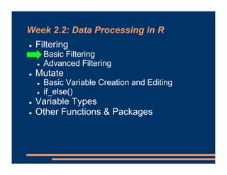
Week 2.2: Data Processing in R
! Filtering
! Basic Filtering
! Advanced Filtering
! Mutate
! Basic Variable Creation and Editing
! if_else()
! Variable Types
! Other Functions & Packages

Filtering Data
! We didn’t see a big difference between
conditions
! But, some RTs look
like outliers—we
may want to
exclude them

Filtering Data
! Often, we want to examine or use just part of
a dataframe
! filter() lets us retain only certain
observations
! experiment %>%
filter(RT < 2000) %>%
group_by(Condition) %>%
summarize(M=mean(RT))
Inclusion criterion: We
want to keep RTs less
than 2000 ms
As we saw last time, this gets the mean RT
for each condition

Filtering Data
! Often, we want to examine or use just part of
a dataframe
! filter() lets us retain only certain
observations
! experiment %>%
filter(RT < 2000) %>%
group_by(Condition) %>%
summarize(M=mean(RT))
Inclusion criterion: We
want to keep RTs less
than 2000 ms

Filtering Data
! This only temporarily filtered the data
! If we want to

Filtering Data
! If we want to run a lot of analyses with this
filter, we may want to save the filtered data as
a new dataframe
! experiment %>%
filter(RT < 2000)
-> experiment.filtered
-> is the assignment
operator. It stores results
or data in memory.
Name of the new dataframe
(can be whatever you want)

Filtering Data
! If we want to run a lot of analyses with this
filter, we may want to save the filtered data as
a new dataframe

Writing Data
! Note that this is just creating a new
dataframe in R
! If you want to save to a folder on your
computer, use write.csv():
! write.csv(experiment.filtered,
file='experiment_filtered.csv')

Filtering Data
! Why not just delete the bad RTs from the
spreadsheet?

Filtering Data
! Why not just delete the bad RTs from the
spreadsheet?
! Easy to make a mistake / miss some of them
! Faster to have the computer do it
! We’d lose the original data
! No documentation of how we subsetted the data

Filtering Data: AND and OR
! What if we wanted only RTs between 200
and 2000 ms?
- experiment %>%
filter(RT >= 200 & RT <= 2000)
! | means OR:
- experiment %>%
filter(RT < 200 | RT > 2000) ->
experiment.outliers
- Logical OR (“either or both”)

Filtering Data: == and !=
! Get a match / equals:
- experiment %>%
filter(TrialsRemaining == 0)
! Words/categorical variables need quotes:
- experiment %>%
filter(Condition=='Implausible')
! != means “not equal to”:
- experiment %>%
filter(Subject != 'S23’)
- Drops Subject “S23”
Note DOUBLE
equals sign

Filtering Data: %in%
! Sometimes our inclusion criteria aren't so
mathematical
! Suppose I just want the “Ducks” and “Panther”
items
! We can check against any arbitrary list:
- experiment %>%
filter(ItemName %in%
c('Ducks', 'Panther'))
! Or, keep just things that aren't in a list:
- experiment %>%
filter(Subject %in%
c('S10', 'S23') == FALSE)

Logical Operators Review
! Summary
- > Greater than
- >= Greater than or equal to
- < Less than
- <= Less than or equal to
- & AND
- | OR
- == Equal to
- != Not equal to
- %in% Is this included in a list?

Mutate
! The last tidyverse function we’ll look at is
mutate()
! Add new variables
! Transform variables
! Recode or rescore variables

Mutate
! We can use mutate() to create new
columns in our dataframe:
- experiment %>%
mutate(ExperimentNumber = 1)
-> experiment
We are creating a column
named ExperimentNumber,
and assigning the value 1 for
every observation
Then, we need to store the
updated data back into our
experiment dataframe

Mutate
! We can use mutate() to create new
columns in our dataframe:
- experiment %>%
mutate(ExperimentNumber = 1)
-> experiment

Mutate
! A more interesting example is where the
assigned value is based on a formula
! experiment %>%
mutate(RTinSeconds = RT/1000)
-> experiment
! For each row, finds the RT in seconds for that
specific trial and saves that into RTinSeconds
- Similar to an Excel formula
• If we wanted to alter the original RT column,
we could instead do:
mutate(RT = RT/1000)

Mutate
! We can even use other functions in
calculating new columns
! experiment %>%
mutate(logRT = log(RT))
-> experiment
! Applies the logarithmic transformation to each
RT and saves that as logRT

if_else()
IF YOU WANT
DESSERT, EAT
YOUR PEAS
… OR ELSE!

if_else()
! if_else(): A function that uses a test to
decide which of two values to assign:
! experiment %>% mutate(
Half=
if_else(
TrialsRemaining >= 15,
1,
2)
) -> experiment
Function name
If 15 or more
trials remain…
“Half” is 1
If NOT, “Half” is 2
A new column
called “Half”--what
value are we going
to assign ?

Which do you like better?
- experiment %>% mutate(
Half=if_else(TrialsRemaining >= 15,
1, 2)) -> experiment
! vs:
- TrialsPerSubject <- 30
Half=if_else(TrialsRemaining >=
TrialsPerSubject / 2, 1, 2)) ->
experiment

Which do you like better?
Half=if_else(TrialsRemaining >= 15,
1, 2)) -> experiment
! vs:
- TrialsPerSubject <- 30
Half=if_else(TrialsRemaining >=
TrialsPerSubject / 2, 1, 2)) ->
experiment
- Explains where the 15 comes from—helpful if we come back
to this script later
- We can also refer to CriticalTrialsPerSubject
variable later in the script & this ensure it’s consistent
- Easy to update if we change the number of trials

if_else()
! Instead of comparing to specific numbers (like
15), we can use other columns or a formula:
RT.Fenced =
if_else(RT < 200, 200, RT))
-> experiment
! What is this doing?

if_else()
RT.Fenced =
if_else(RT < 200, 200, RT))
-> experiment
! Creates an RT.Fenced column where:
! Where RTs are less than 200 ms, replace them
with 200
! Otherwise, use the original RT value
! i.e., replace all RTs less than 200 ms with the
value 200

if_else()
RT.Fenced =
if_else(RT < 200, 200, RT))
-> experiment
! For even more complex rescoring, use
case_when()

Types
! R treats continuous & categorical variables
differently:
! These are different data types:
- Numeric
- Character: Freely entered text (e.g.,
open response question)
- Factor: Variable w/ fixed set of
categories (e.g., treatment vs. placebo)

Types
! R’s current heuristic when reading in data:
- No letters, purely numbers → numeric
- Letters anywhere in the column →
character

Types: as.factor()
! For variables with a fixed set of categories, we
may want to convert to factor
! experiment %>%
mutate(Condition=as.factor(Condition))
-> experiment

Types: as.numeric()
! Age was read as a character variable because
some people “Declined to report”
! But, we may want to treat it as numeric despite
this

Types: as.numeric()
! Age was read as a character variable because
some people “Declined to report”
- experiment %>%
mutate(AgeNumeric=as.numeric(Age)) ->
experiment
• We now get quantitative
information on Age
• Values that couldn’t be turned
into numbers are listed as NA
• NA means missing data--we’ll
discuss that more later in the term

Other Functions
! Some built-in analyses:
! aov() ANOVA
! lm() Linear regression
! glm() Generalized linear models (e.g., logistic)
! cor.test() Correlation
! t.test() t-test

Other Packages
! Some other relevant packages:
! lavaan Latent variable analysis and
structural equation modeling
! psych Psychometrics (scale construction, etc.)
! party Random forests
! stringr Working with character variables
! lme4: Package for linear mixed-effects models
! Get this one for next week

Getting Help
! Get help on a specific known function:
- ?t.test
- Lists all
arguments
! Try to find a
function on a
particular topic:
- ??logarithm

Mixed Effects Models - Data Processing

Empfohlen

Empfohlen

Weitere ähnliche Inhalte

Was ist angesagt?

Was ist angesagt? (20)

Ähnlich wie Mixed Effects Models - Data Processing

Ähnlich wie Mixed Effects Models - Data Processing (20)

Mehr von Scott Fraundorf

Mehr von Scott Fraundorf (7)

Kürzlich hochgeladen

Kürzlich hochgeladen (20)

Mixed Effects Models - Data Processing