Economic pipe size
•
2 gefällt mir•873 views

To determine the optimum pipe diameter, you should go make the comparative analysis to determine the most optimum pipe size which reflects the most economic option. This example is for illustration the importance of the the comparative analysis. Note: According to ASME, pipe with 5 in diameter is not standard, but i selected it in the example for illustration only.

Empfohlen
Weitere ähnliche Inhalte
Was ist angesagt?
Was ist angesagt? (20)
Ähnlich wie Economic pipe size
Ähnlich wie Economic pipe size (20)
Mehr von Mohamed A. Hassan, CEng MIChemE
Mehr von Mohamed A. Hassan, CEng MIChemE (13)
Kürzlich hochgeladen
Kürzlich hochgeladen (20)
Economic pipe size
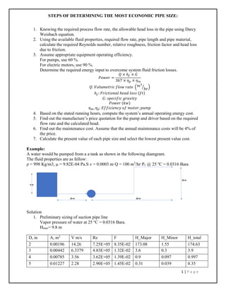
- 1. STEPS OF DETERMINING THE MOST ECONOMIC PIPE SIZE: 1 | P a g e 1. Knowing the required process flow rate, the allowable head loss in the pipe using Darcy Weisbach equation. 2. Using the available fluid properties, required flow rate, pipe length and pipe material, calculate the required Reynolds number, relative roughness, friction factor and head loss due to friction. 3. Assume appropriate equipment operating efficiency. For pumps, use 60 %. For electric motors, use 90 %. Determine the required energy input to overcome system fluid friction losses. 𝑃𝑜𝑤𝑒𝑟 = 𝑄 × ℎ 𝑓 × 𝐺 367 × 𝜂 𝑝 × 𝜂 𝑚 𝑄: 𝑉𝑜𝑙𝑢𝑚𝑒𝑡𝑟𝑖𝑐 𝑓𝑙𝑜𝑤 𝑟𝑎𝑡𝑒 ( 𝑚3 ℎ𝑟⁄ ) ℎ 𝑓: 𝐹𝑟𝑖𝑐𝑡𝑖𝑜𝑛𝑎𝑙 ℎ𝑒𝑎𝑑 𝑙𝑜𝑠𝑠 (𝑓𝑡) 𝐺: 𝑠𝑝𝑒𝑐𝑖𝑓𝑖𝑐 𝑔𝑟𝑎𝑣𝑖𝑡𝑦 𝑃𝑜𝑤𝑒𝑟 (𝑘𝑤) 𝜂 𝑚, 𝜂 𝑝: 𝐸𝑓𝑓𝑖𝑐𝑖𝑒𝑛𝑐𝑦 𝑜𝑓 𝑚𝑜𝑡𝑜𝑟, 𝑝𝑢𝑚𝑝 4. Based on the stated running hours, compute the system’s annual operating energy cost. 5. Find out the manufacture’s price quotation for the pump and driver based on the required flow rate and the calculated head. 6. Find out the maintenance cost. Assume that the annual maintenance costs will be 4% of the price. 7. Calculate the present value of each pipe size and select the lowest present value cost. Example: A water would be pumped from a a tank as shown in the following diamgram. The fluid properties are as fellow: ρ = 998 Kg/m3, µ = 9.82E-04 Pa.S, ɛ = 0.0003 m, Q = 100 m3 /hr, Pv @ 25 o C = 0.0316 Bara Solution 1. Preliminary sizing of suction pipe line Vapor pressure of water at 25 o C = 0.0316 Bara. Hmax= 9.8 m D, in A, m2 V m/s Re F H_Major H_Minor H_total 2 0.00196 14.26 7.25E+05 8.35E-02 173.08 1.55 174.63 3 0.00442 6.3379 4.83E+05 1.32E-02 3.6 0.3 3.9 4 0.00785 3.56 3.62E+05 1.39E-02 0.9 0.097 0.997 5 0.01227 2.28 2.90E+05 1.45E-02 0.31 0.039 0.35 10 m 20 m 4 m 10 m
- 2. STEPS OF DETERMINING THE MOST ECONOMIC PIPE SIZE: 2 | P a g e Liquid velocities in straight pipe in excess of 4.6 m/s will generally produce objectionable noise. Where there are numerous bends, valves, the velocity limit for noise may be in the order of 3 m/s. The preliminary pipe diameter should be 4 in. Assume that the discharge pipe diameter is like the suction. D, in H_Major H_minor H_total 4 11.8 0.097 11.9 5 10.61 0.039 10.65 So, we would select 4, 5 in to enter to the economic analysis of the pipe The pump should be selected according to the following criteria: Flow rate = 100 m3 /h Required flow head = 12,8 m 2. Economic analysis of suction pipeline Note: The prices assumed here are only for illustration • Calculate the pump power: D, in Power, KW 4 6.49 5 5.5 Assume the energy power 1 $/KWh Thus, the annual energy cost based on 8000 hrs yearly: D, in Cost, $ 4 51,920 5 44,000 • Here, I assume the capital cost of the pump is 13,000 $. • The maintenance cost = 520 $ Thus, the annual cost: D, in Annual cost, $ 4 52,440 5 44,520 • Estimate the total capital cost D, in Labor cost, $ 4 30,000 5 50,000 • Break-even analysis: 𝑛 𝑒 = 50,000 − 30,000 52,440 − 44,520 = 2.5 𝑦𝑟
- 3. STEPS OF DETERMINING THE MOST ECONOMIC PIPE SIZE: 3 | P a g e • Estimate the total life cycle cost: D, in Present value, $ 4 574,309 5 512,102 So, the optimum economic pipe diameter is 5 in. Summary of Economic variables for two pipe systems Parameter 4 in 5 in Fluid velocity m/s 3.56 2.28 Reynolds number 3.62E+5 2.9E+5 Head loss due to friction, m 11.9 10.65 Power, KW 6.49 5.5 Annual cost, $ 52,440 44,520 Initial capital cost, $ 30,000 50,000 Life cycle present value, $ 574,309 512,102 Conclusion: What is appeared from the first glance that the optimum diameter is the smallest diameter with smallest initial cost, but what is appeared economically is that the 5 in pipe is optimum economically. Hint: All the cost and prices are for illustration only and not actual. Break-even analysis: 𝑛 𝑒 = 𝐷𝑖𝑓𝑓𝑒𝑟𝑒𝑛𝑐𝑒 𝑖𝑛 𝑐𝑎𝑝𝑖𝑡𝑎𝑙 cos𝑡 𝐷𝑖𝑓𝑓𝑒𝑟𝑒𝑛𝑐𝑒 𝑖𝑛 𝑜𝑝𝑒𝑟𝑎𝑡𝑖𝑛𝑔 cos𝑡 Total life cycle cost present value: 𝐶 = 𝐶𝑖 + 𝐶0 (1 + 𝑖) 𝑛 − 1 𝑖(1 + 𝑖) 𝑛 Ci: initial capital cost, $ Co: operating cost i: interest rate n: total life time