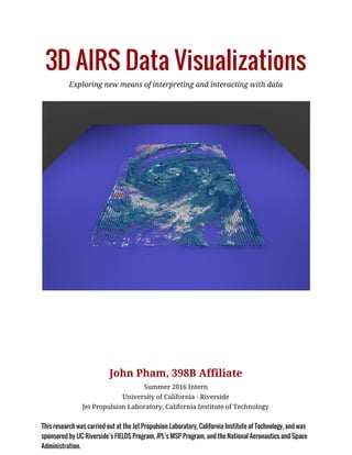
1. 3D AIRS Data Visualizations
Exploring new means of interpreting and interacting with data
John Pham, 398B Affiliate
Summer 2016 Intern
University of California - Riverside
Jet Propulsion Laboratory, California Institute of Technology
This research was carried out at the Jet Propulsion Laboratory, California Institute of Technology, and was
sponsored by UC Riverside’s FIELDS Program, JPL’s MSP Program, and the National Aeronautics and Space
Administration.

2. Table of Contents
Abstract
Overview
The Program
File Conversions
Creating a 3D model
Optimization in Generating the 3D Model
Current Spatial Approach
Volumetric-Photorealistic Clouds
Comparing Data
Animations
Augmented/Virtual Reality Applications
Future Direction
Conclusion
References
Acknowledgements
Evan Manning
Appendix
Granule 033 - 09/06/2006
Demonstrating variability of cloud densities
Granule 192 - 09/22/2002
Early Render with Aqua Satellite
1

3. Abstract
The goal of this project is to develop a new, streamlined method to visualize and
interact with data in 3D. AIRS cloud data is used as a starting point. The technologies
used to in this project is Python, Blender, Unity, HTML, CSS, Javascript, and Adobe
Premier. Python is used to convert the data from HDF-EOS to Pickle which Python can
easily interface with. Blender has a Python wrapper which makes scripting the
creation of the 3D models in Blender straightforward. Use of volumetric “fluffy” clouds
and cylinders have been tried but the decision was made to stay with cylinders due to
them being a better representation of the data. Within Blender, a color scheme can be
determined such as cloud phase, type, and many more. Once a 3D mesh is created in
Blender, porting over to Unity or a web viewer is easy. At the time of the end of the
internship, a base program is created where scientists and others interested can use
with ease.
Overview
The Atmospheric Infrared Sounder (AIRS) is a hyperspectral infrared sounder which
was launched onboard the Earth Observing Satellite (EOS), Aqua in May of 2002 with a
sun-synchronous 1:30PM polar orbit. Since its launch, AIRS has retrieved over 13 years
worth of data in 2,378 channels ranging from surface temperature to clouds.
Retrieval pattern: NASA GES DISC
The instrument retrieves data in a “whisk-broom” scan pattern in 90 Fields of View
(FOVs) every 2.67 seconds. Each FOV is about 15 KM nadir and increases in size when
scanning toward the edge due to the angle.
2

4. Granule map: NASA JPL - AIRS
The data is packaged into 240 6-minute granules per day with each granule containing
90 FOVs with each containing 135 scans. This means each granule can be plotted as a
90 by 135 rectangle with up to 12,150 data points.
Single granule: Generated using MatPlotLib
AIRS scientists typically generate their own version with their own code of 2D visuals
to conduct their science. Taking cloud products as an example, these visuals can
include cloud top temperature, effective cloud fraction, and many more fields.
3

5. 2D view: NASA JPL - Bill Irion
These visuals do portray the data in a easy to understand way, but the number of
relationships to visualize is limited due to it being graphed in 2D space. The visual
above shows three relationships: longitude, latitude, and classification. Introducing
another axis will increase the visible relationships from three to seven.
3D view: Generated in Blender
With a 3D visual, the relationships of not only longitude, latitude, and classification is
shown but also: longitude depth, latitude depth, Z-depth, and object density.
4

6. The Program
Program layout
The main visualizer program that has been developed is currently on its 7th iteration.
Written in Python and to be used with Blender, it can read data in Hierarchical Data
Format - Earth Observing System (HDF-EOS) converted to Python Pickle format to
generate a 3D model of the system. Different parameters can then be applied to the
model such as color scheme, animations, data comparison and live interaction if
imported into Unity.
File Conversions
The reasoning for converting the native data files from HDF-EOS to Python Pickle is
because Blender, which has a built in version of Python 3, does not currently have any
HDF-EOS reader. To surpass this, a script was written in Python 2.7 which converts the
HDF-EOS files to Pickle files which Python 3 can easily interface with.
5

7. Creating a 3D model
Model view in Blender
Once the conversion from HDF-EOS to Pickle has been done, the built in version of
Python in Blender can easily interface with the data. For these preliminary renders,
the fields we are using are: Latitude, Longitude, Effective Cloud Fraction, Cloud Top
Pressure, and Cloud Phase. These values are read for each scan to generate a cylinder
in Blender. Once a cylinder is created, a material is applied based on the chosen color
scheme. This is done for the rest of the granule.
Optimization in Generating the 3D Model
Terminal prompt of the program creating cylinders
There are various ways of generating objects within Blender. The most memory
intensive is creating a new mesh and corresponding data for each object. This method
was initially used to generate the 3D model which resulted in modeling times taking up
to 3 hours.
The approach used to reduce the modeling time was to create a mesh and data for the
first scan then for all following scans, copy the mesh but alter its data instead of
creating a new mesh and associating data for each scan. By doing this, the modeling
time was reduced to around 100 ± 60 seconds depending on the complexity of the
granule.
6

8. Current Spatial Approach
Graph generated based on paper published by Miller et al.
Based on a paper published by Miller et al., the approach to scaling the cylinders is to
use the predicted cloud type which is figured out by comparing the scan’s cloud top
pressure and effective cloud fraction to determine its depth.
Volumetric-Photorealistic Clouds
Volumetric-Photorealistic clouds: Generated in Blender
One goal of the project is to produce photorealistic representations from the cloud data
to be used for outreach. A problem that came up was the time it would take to generate
these renders due to the hardware being used. These types of renders are possible but
not on the machines that were being used at the time.
7

9. Clouds wireframe and rendered views showing Z-Fighting in Blender
Another problem that had come up was a issue prevalent in 3D modeling, Z-Fighting.
The module that was being used is called Cloud Generator, a open source module for
Blender. The way the volumetric clouds are generated with the module is that it takes
the mesh of an object, in our case a cylinder, and creates a gaussian distribution of
volume points with a 50% tolerance. Due to such a large tolerance, Z-Fighting was
prevalent so changes were made in the module to limit the possible Z-Fighting. The
changes were pushed to the repository and accepted.
Comparing Data
Comparing AIRS data with MODIS/CloudSat
Another use for the program is to compare different data sets. For this preliminary
demo, a image of CloudSat/MODIS was used to compare with AIRS data.
8

10. Animations
The program can also create animations with styles being limitless. Some examples
have been: phasing between two different retrieval algorithms to highlight differences,
360 animation to show a granule in full coverage, and a 2D to 3D view conversion
highlighting what a 3D visual can show.
Augmented/Virtual Reality Applications
Left: Unity Right: Web viewer
One of the key features of Blender is its ability to export into a multitude of file formats
many of which is usable in Unity. The application of VR has been explored and a
preliminary demo of using a Google Cardboard, web player, and the start exporting to
more advanced VR headsets has started.
Future Direction
Left: View of 1 granule in Blender Right: Artist’s representation of clouds
9

11. The future goal is to be able to create global renders, ensure a true representation of
the data, AR/VR adoption, and return back to the photorealistic clouds.
Conclusion
The development of this program lays out a foundation where other scientists can use
to visualize and interact with their data in a whole new way. 3D visuals contain more
information and hides little if any data due to it not being condensed into 2D. As
shown above, the adaption of the output of this program can be easily integrated into a
AR/VR application which adds an entire new dimension of visualizing and interacting
with the data.
10

12. References
Aumann, H. H., Chahine, M. T., Gautier, C., Goldberg, M., Kalnay, E., McMillin, L.,
Revercomb, H., Rosenkranz, P. W., Smith, W. L., Staelin, D. H., Strow, L. and
Susskind, J., "AIRS/AMSU/HSB on the Aqua Mission: Design, Science Objectives,
Data Products and Processing Systems," IEEE Trans. Geosci. Remote Sensing, 41,
253-264 (2003).
Miller, S. D., and Coauthors, 2014: Estimating three-dimensional cloud structure via
statistically blended satellite observations. J. Appl. Meteor. Climatol., 53,
437–455, doi:10.1175/JAMC-D-13-070.1.
S. L. Nasiri, B. H. Kahn, and H. Jin, "Progress in Infrared Cloud Phase Determination
Using AIRS," in Advances in Imaging, OSA Technical Digest (CD) (Optical Society
of America, 2009), paper HWA3.
Acknowledgements
Evan Manning
My mentor, being his first intern he did everything in his position to enable me for my
internship. He was able to answer every question I had with more to note. His
experience and expertise shows in everything he does.
UC Riverside FIELDS Program
Thanks to their securement of the NASA MIRO Grant, I was able to be funded for my
internship.
Brian Kahn
The cloud expert. He has given insight on how to create visuals that will enhance
science.
Sun Wong and Tau Wang
Sharing their methods in analyzing CloudSat and MODIS data.
Government sponsorship acknowledged
11

13. Appendix
Granule 033 - 09/06/2006
Left Column: Colored by phase Right Column: Colored by type
Demonstrating variability of cloud densities
12

14. Granule 192 - 09/22/2002
Left Column: Colored by phase Right Column: Colored by type
Early Render with Aqua Satellite
13

15. Additional still and animated renders along with the program to create the renders
may be requested. Contact Evan Manning (​Evan.M.Manning@jpl.nasa.gov​) or John
Pham (​johnpham@engineer.com​)
14