Volume 13, Issue 4 Ver. II (Jul. - Aug. 2016)

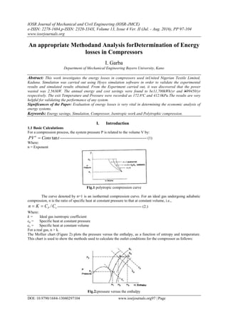
1. IOSR Journal of Mechanical and Civil Engineering (IOSR-JMCE)
e-ISSN: 2278-1684,p-ISSN: 2320-334X, Volume 13, Issue 4 Ver. II (Jul. - Aug. 2016), PP 97-104
www.iosrjournals.org
DOI: 10.9790/1684-13040297104 www.iosrjournals.org97 | Page
An appropriate Methodand Analysis forDetermination of Energy
losses in Compressors
I. Garba
Department of Mechanical Engineering Bayero University, Kano
Abstract: This work investigates the energy losses in compressors used inUnited Nigerian Textile Limited,
Kaduna. Simulation was carried out using Hysys simulation software in order to validate the experimental
results and simulated results obtained. From the Experiment carried out, it was discovered that the power
wasted was 2.563kW. The annual energy and cost savings were found to be11,700kWh/yr and N99450/yr
respectively. The exit Temperature and Pressure were recorded as 172.8ºC and 412.0kPa.The results are very
helpful for validating the performance of any system.
Significances of the Paper: Evaluation of energy losses is very vital in determining the economic analysis of
energy systems.
Keywords: Energy savings, Simulation, Compressor, Isentropic work and Polytrophic compression.
I. Introduction
1.1 Basic Calculations
For a compression process, the system pressure P is related to the volume V by:
tConsPVn
tan -------------------------------------------------------------------- (1)
Where:
n = Exponent
Fig.1 polytropic compression curve
The curve denoted by n=1 is an isothermal compression curve. For an ideal gas undergoing adiabatic
compression, n is the ratio of specific heat at constant pressure to that at constant volume, i.e.,
vP CCKn / ------------------------------------------------------------------ (2.)
Where:
k = Ideal gas isentropic coefficient
cp = Specific heat at constant pressure
cv = Specific heat at constant volume
For a real gas, n > k.
The Mollier chart (Figure 2) plots the pressure versus the enthalpy, as a function of entropy and temperature.
This chart is used to show the methods used to calculate the outlet conditions for the compressor as follows:
Fig.2:pressure versus the enthalpy

2. An appropriate Methodand Analysis forDetermination of Energy losses in Compressors
DOI: 10.9790/1684-13040297104 www.iosrjournals.org98 | Page
Figure 3 Typical Mollier chart for compression
A flash is performed on the inlet feed at pressure P1, and temperature T1, using a suitable K-value and
enthalpy method. The entropy S1, and enthalpy H1 are obtained and the point (P1, T1, S1, H1) are obtained.
The constant entropy line through S1 is followed until the user-specified outlet pressure is reached. This point
represents the temperature (T2) and enthalpy conditions (H2) for an adiabatic efficiency of 100%. The adiabatic
enthalpy change ∆Had is given by:
12 HHHad  --------------------------------------------------------------------- (3)
 If the adiabatic efficiency, ad, is given as a value less than 100 %, the actual enthalpy change is calculated
from:
ad
ad
ac
H
H

 ------------------------------------------------------------- (4)
 The actual outlet stream enthalpy is then calculated using:
acHHH  13 H3-------------------------------------------------------- (5)
 Point 3 on the Mollier chart, representing the outlet conditions is then obtained. The phase split of the outlet
stream is obtained by performing an equilibrium flash at the outlet conditions.
 The isentropic work (Ws) performed by the compressor is computed from:
JHJHHW acs  )( 13 ---------------------------------------------- (6)
Where:
J = mechanical equivalent of energy
The isentropic power required is:
33000
778
F
HGHP adad  -------------------------------------------------------- (7)
ad
ad
acac
GHPF
HGHP


33000
778 ----------------------------------------------- (8)
778 HHEADad ---------------------------------------------------------------- (9)
Where:
GHP= work, hP
∆H = enthalpy change,
F =mass flow rate,
HEADad =Adiabatic Head,
The factor 33000 is used to convert the units into horsepower.
The isentropic and polytropic coefficients, polytropic efficiency, and poly tropic work can be calculated using
one of the two methods; the method from the GPSA Engineering Data Book, and the method from the ASME
Power Test Code 10.
ASME Method
This method is more rigorous than the default GPSA method, and yields better results over a wider range of
compression ratios and feed compositions.
For a real gas, as previously noted, the isentropic volume exponent (also known as the isentropic coefficient), ns,
is not the same as the compressibility ratio, k. The ASME method distinguishes between k and ns for a real gas.

3. An appropriate Methodand Analysis forDetermination of Energy losses in Compressors
DOI: 10.9790/1684-13040297104 www.iosrjournals.org99 | Page
Adiabatic Efficiency Given
In this method, the isentropic coefficient nsis calculated as:
)/ln(/)/ln( 2112 VVPPns  ------------------------------------------------------------- (10)
Where:
V1 = Volume at the inlet conditions
V2 = Volume at the outlet pressure and inlet entropy conditions
P1= Pressure at the inlet conditions
P2= Pressure at the outlet conditions
The compressor work for a real gas is calculated from equation (2.8), and the factor from the following
relationship:
]1)/[()]1/([144 /)1(
1211   ss nn
ssac PPVPfnnW ----------------------------- (11)
The ASME factor f is usually close to 1. For a perfect gas, f is exactly equal to 1, and the isentropic coefficient
nsis equal to the compressibility factor k.
The polytropic coefficient, n, is defined by:
)/ln(/)/ln( 2112 VVPPn  --------------------------------------------------------------- (12)
The polytropic work, i.e., the reversible work required to compress the gas in a polytropic compression process
from die inlet conditions to the discharge conditions is computed using:
}1
1
){(
)1
(144 1211 




n
n
PPVPf
n
n
Wp -------------------------------------- (13)
Where:
Wp = polytropic work
For ideal or perfect gases, the factor f is equal to 1. The polytropic efficiency is then calculated by:
p
s
p
W
W
 p------------------------------------------------------------------------- (14)
Where Ws = isentropic work
This polytropic efficiency will not agree with the value calculated using the GPSA method which is computed
using p = {(n-l)/n) / {(k-l)/k}.
GPSA Method
This GPSA method is the default method, and is more commonly used in the chemical process industry [9].
In this method, the adiabatic head is calculated from equations above. Once this is calculated, the isentropic
coefficient k is computed by trial and error using:
}1))}{1/{(/){( /)19
1
2
121   kk
ac
P
P
kRTZZHEAD [39]-------------------------(15)
Where:
Z1, Z2 = compressibility factors at the inlet and outlet conditions
R = gas constant
T1 = temperature at inlet conditions.
This trial and error method of computing k produces inaccurate results when the compression ratio,
becomes low. If the calculated compression ratio is less than a value set by the user, the value of k has to be
calculated.If k does not satisfy 1.0 < k < 1.66667, the isentropic coefficient, is calculated by trial and error based
on the following:
kk
PPTZZT /)1(
121212 )/[()/( 
 ---------------------------------------------- (16)
The polytrophic compressor equation is given by:
}1)/}]{(/)1/{(]2/)[( /)1(
12121   nn
p PPnnRTZZHEAD
Where Headp is polytrophic head
The adiabatic head is related to the polytropic head by:
p
p
ad
ad
HEADHEAD

 ------------------------------------------------------------------- (17)
The polytrophic efficiency n is calculated by:

4. An appropriate Methodand Analysis forDetermination of Energy losses in Compressors
DOI: 10.9790/1684-13040297104 www.iosrjournals.org100 | Page
)]1/(/[)]1/([  kknnp p------------------------------------------------------ (18)
The polytropic coefficient, n, the polytropic efficiency p, and the polytropic head are determined by trial and
error method. The polytropic gas horsepower is then given by:
33000
F
HEADGHP pp  ]-----------------------------------------------------(19)
II. Material And Methods
The entropy data needed for these calculations are obtained from a number of entropy calculation
methods. These include die Soave-Redlich-Kwong cubic equation of state, and the Curl-Pitzer correlation
method. Thermodynamic systems may be used to generate entropy data. User-added subroutines may also be
used to generate entropy data.Once the entropy data are generated, the condition of the outlet conditions from
the compressor and the compressor power requirements are computed, using either a user-input adiabatic or
polytrophic efficiency.
III. Results And Discussion
Table 1: Air Facility Reading for 75KI01
Time Air Inlet
Temp.(0
c)
Oil Cooler
L/D Temp
(0
c)
Oil Cooler
L/D
Outlet (0
c)
After Cool
Air Outlet
Temp. (0
c)
Turbine
Inlet Steam
Temp. (0
c)
Turbine Inlet
Steam Pressure
(N/M2
)
Turbine Exhaust
Pressure (N/M2
)
8:00 Hr 32 52 30 34 400 41 17.1
9:00 Hr 30 52 32 34 400 41 17.2
10:00 Hr 32 53 31 34 400 42 17.3
11:00 Hr 30 53 31 34 400 42 16.9
12:00 Hr 33 52 32 34 400 42 17.0
13:00 Hr 32 51 32 34 400 41 17.2
14:00 Hr 33 51 32 34 400 41 17.3
15:00 Hr 33 51 30 34 400 41 17.2
16:00 Hr 33 52 32 34 400 42 17.2
17:00 Hr 33 52 31 34 400 42 17.3
18:00 Hr 33 52 32 34 400 42 17.3
Average 32.4 51.9 31.4 34 400 41.5 17.2
Compressor Heat Loss
Assumption: air is an ideal gas. Steady operating condition exists. There is pressure losses:
 
 


















1
1
1
1
21
,
n
n
comp
incomp
P
P
n
nRT
W

----------------------------- (20)
 
 
 
KgKJW incomp
/9.2961
101
801
14.18.0
293287.04.1 4.1
4.0
,



















A = D2
/4 = (3 x 10-3
m2
)/4 = 7.069 x 10-6
m2
Air leaking through the hole is determined to be
 
line
line
line
k
edischair
T
K
KRA
RT
P
K
Cm 





















1
2
1
2 1
1
arg
= 0.008632kg/s
 
297
14.1
2
287.04.110069.7
297287.0
801
14.1
2
65.0 6
14.1
1





















 

airm

5. An appropriate Methodand Analysis forDetermination of Energy losses in Compressors
DOI: 10.9790/1684-13040297104 www.iosrjournals.org101 | Page
Then the power wasted by the leaking compressed air becomes
incompair
WmwastedPower ,
 -------------------------------------- (21)
= 0.008632 x 296.9
= 2.563kW
The compressor operates for 4200 hours a year, and the motor efficiency is 0.92.
Then the annual energy and cost savings are:
Energy savings = power saved x operating hours
motor
= 2.563kW x 4200
0.92
= 11,700kWh/yr
Cost savings = (energy savings) x (unit cost of energy)
= 11700 x N8.50k/wh
= N99450/yr
Compressor Simulation Results:
Table 2: compressor simulation
S/No Simulated Parameters Simulated Values
1. Duty (kW) 5.0684e+02
2. Polytropic Exponential 1.626
3. Adiabatic Efficiency 71.72
4. Adiabatic Head (m) 7586
5. Isentropic Exponential 1.402
6. Polytropic Efficiency 74.26
7. Polytropic Head (m) 7852
8. Polytropic Head Factor 1.000
Table 3: Compressor Rating Curves
S/NO. Flow (ACT m3
/h) Head (m) Efficiency (%)
1. 7812 7680 69.20
2. 8388 7575 72.00
3. 8964 7841 72.48
4. 9504 7347 72.58
5. 1.008e+004 7153 73.08
6. 1.062e+004 6717 72.46
7. 1.120e+004 5858 69.39
8. 1.148e+004 4957 62.91
Table 4: Compressor Flow Limits
S/NO. Flow Limits
1. Surge Curve: Inactive
2. Speed Flow
3. Stone Wall Curve: Inactive
4. Field Flow Rate (ACT_m3
/h) 8330
5. Stone Wall Flow ---
6. Compressor Volume (m3
) 10.00
7. Rotational inertia (kg/m2
) 6.000
8. Radius of gyration (m) 0.2000
9. Mass (kg) 150.0
10. Friction loss factor (rad/min) 3.000
Table 5: Compressor inlet Conditions
Overall
Vapour/Phase Fraction 1.0000
Temperature: (0
C) 70.00
Pressure: (kPa) 208.0
Molar Flow (kgmol/h) 607.7
Mass Flow (kg/h) 1.759e+004
Std Ideal LiqVol Flow (m3
/h) 20.00
Molar Enthalpy (kJ/kgmol) 1283
Mass Enthalpy (kJ/kg) 44.32
Molar Entropy (kJ/kgmol-0
C) 116.2
Mass Entropy (kJ/kg-0
C) 4.015

6. An appropriate Methodand Analysis forDetermination of Energy losses in Compressors
DOI: 10.9790/1684-13040297104 www.iosrjournals.org102 | Page
Heat Flow (kJ/h) 7.797e+005
Molar Density (kgmol/m3
) 7.295e-002
Mass Density (kg/m3
) 2.112
Std Ideal Liq Mass Density (kg/m3
) 879.6
Molar Heat Capacity (kJ/kgmol-0
C) 29.00
Mass Heat Capacity (kJ/kg-0
C) 1.002
Thermal Conductivity (W/m-K) 2.775e-002
Viscosity (cP) 2.093e-002
Molecular Weight 28.95
Z Factor 0.9994
Cp/Cv 1.406
Act. Vol. Flow (m3/h) 8330
Table 6: Compressor Outlet Conditions
Overall
Vapour/Phase Fraction 1.0000
Temperature: (0
C) 172.8
Pressure: (kPa) 412.0
Molar Flow (kgmol/h) 607.7
Mass Flow (kg/h) 1.759e+004
Std Ideal LiqVol Flow (m3
/h) 20.00
Molar Enthalpy (kJ/kgmol) 4286
Mass Enthalpy (kJ/kg) 148.0
Molar Entropy (kJ/kgmol-0
C) 118.2
Mass Entropy (kJ/kg-0
C) 4.083
Heat Flow (kJ/h) 2.604e+006
Molar Density (kgmole/m3
) 0.1111
Mass Density (kg/m3
) 3.215
Std Ideal Liq Mass Density (kg/m3
) 879.6
Molar Heat Capacity (kJ/kgmol-0
C) 29.60
Mass Heat Capacity (kJ/kg-0
C) 1.023
Thermal Conductivity (W/m-K) 3.421e-002
Viscosity (cP) 2.524e-002
Molecular Weight 28.95
Z Factor 1.000
Cp/Cv 1.395
Act. Vol. Flow (m3
/h) 5471
Table 7:Compressor Sizing Input Details
Unit operation type: Compressor
Equipment type: Gas Compressor – Centrifugal Horizontal
Compressor sizing input Details
Operating capacity 17591.48kg/h
Operating adiabatic head 7585.53m
Operating polytropic head 7852.30m
Adiabatic efficiency 71.7188
Polytropic efficiency 74.2551
Operating gas power 506.84 kW
Capacity overdesign factor 1,1000
Head overdesign factor 1,1000
Table 8: Compressor Sizing Data Output
Unit operation type: Compressor
Equipment type: Gas Compressor – Centrifugal Horizontal
Compressor sizing input Details
Design capacity 19350.63kg/h
Design adiabatic head 8344.1m
Design polytropic head 8637.5m
Gas power 613.16kW
Mechanical losses 10.93kW
Design power 624.09kW
Driver power 900hp

7. An appropriate Methodand Analysis forDetermination of Energy losses in Compressors
DOI: 10.9790/1684-13040297104 www.iosrjournals.org103 | Page
Figure .4: Compressor
Figure 5: Head Curves of the Compressor

8. An appropriate Methodand Analysis forDetermination of Energy losses in Compressors
DOI: 10.9790/1684-13040297104 www.iosrjournals.org104 | Page
Fig. 6: Variation of Efficiency with Flow
IV. Discussion Of Results
Simulated Results
From figure 6 (efficiency curves of the compressor) the efficiency increases when the flow (m3
/h) is
high and reduces when the level of the flow (m3
/h) decreases.
From table 2 the adiabatic efficiency was found to be 71.7% while the polytrophic efficiency was 74.3%.
Also from table 4 (compressor flow limits) the friction loss factor was found to be 3.00 rad/min.
From the head curves of the compressor (figure 5), the head decreases when the flow (m3
/h) increases.
The efficiency increases when the flow (m3
/h) increases as shown in figure 6.
V. Conclusion
This work set out to achieve the main goal of exploring ways for an effective energy saving which is
expected to reduce energy cost, generate higher profit and increase capacity utilization. Energy loss which
affects the output of the system was minimized. The empirical process heat loss, the actual values heat loss and
the simulation model heat losss were found to be 2.56Kw, ,9.81kW and 10.93kW. The adiabatic efficiency and
polytropic efficiency were found to be 71.7188% and 74.2551%. Moreover, the mechanical losses was found to
be 10.93kW.
References
[1]. Emshoff, J. R (2001)."Design and use of computer simulation Models". New York: Macmillan,
[2]. Chilton, C. H.(2002)"Cost Engineering in the Process Industries". New York: McGraw – Hill,
[3]. Engeda, Abraham (1999). "From the Crystal Palace to the pump room".Mechanical Engineering.ASME.
[4]. Elliott Company. "Past, Present, Future, 1910-2010"(PDF). Elliott. Retrieved 1 May 2011.
[5]. API ( 2002). Std 673-2002 Centrifugal Fans for Petroleum, Chemical and Gas Industry Services. New York: API.
[6]. Whitfield, A. & Baines, N. C. (1990).Design of Radial Turbomachinery.Longman Scientific and Technical.ISBN 0-470-21667-0.
[7]. Aungier, Ronald H. (2000). Centrifugal Compressors, A Strategy for Aerodynamic Design and Analysis. ASME Press. ISBN 0-
7918-0093-8.
[8]. Saravanamuttoo, H.I.H., Rogers, G.F.C. and Cohen, H. (2001).Gas Turbine Theory.Prentice-Hall.ISBN 0-13-015847-X.
[9]. Baines, Nicholas C. (2005). Fundamentals of Turbocharging. Concepts ETI .
[10]. . SAE/standards/power and propulsion/engines.SAE International.Retrieved 23 April 2011.
[11]. API ( 2002). Std 617-2002 Axial and Centrifugal Compressors and Expander-compressors for Petroleum, Chemical and Gas
Industry Services. New York: API.
[12]. ASHRAE, American Society of Heating, Refrigeration and Air-Conditioning Engineers."Standards &
Guidelines"ASHRAE.Retrieved 23 April 2011.
[13]. API ( 2007). Std 672-2007 Packaged, Integrally Geared Centrifugal Air Compressors for Petroleum, Chemical, and Gas Industry
Services. New York: API.