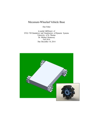
1. Mecanum-Wheeled Vehicle Base
Dan Fisher
in partial fulfillment of
ETLS 789 Simulation and Visualization of Dynamic Systems
University of St. Thomas
Dr. Michael Hennessey
Fall 2014
Due December 18, 2014

2. Abstract
Mecanum wheels offer a means to implement omni-directional translational motion in a vehicle
platform. As the wheel rotates, rollers around its circumference create a force directed at an
angle relative to the plane of rotation. Various combinations of wheel rotational velocities can
provide a net force in any direction. This provides enhanced maneuverability in close quarters,
but is often limited to smoother surfaces as the wheels require many moving rollers that can
become easily obstructed by debris. Applications of this model run from small hobby kits up to
heavy duty industrial vehicles. This project presents the simulation of a typical four mecanum-
wheeled vehicle platform using MATLAB and Simulink. All modes of vehicle motion are
simulated and animated using frame-by-frame capture of a 3D vehicle model in Solidworks.
System Equations
The system equations presented here are the work of Lin & Shih [1], with modifications as
indicated.
Mecanum Wheel Parameters
Each wheel is mounted on a vehicle chassis with a local robot frame of reference {R}: XRYRZR
with the origin at the geometric center G and the wheel’s center at A.
The key parameters for each wheel are
 the angle of GA relative to the XR
axis,  the angle of the wheel’s axle
relative to GA, and  the angle of the
rollers’ axles relative to the wheel’s
plane of rotation. Note that these
parameters vary for each wheel on the
vehicle.
The wheel’s angular velocity 𝜑̇ is
defined positively for clockwise (CW)
rotation looking outward from the
vehicle base.
Vehicle Base Configuration
Figure 2 shows the vehicle base as viewed from above. The rollers shown are those touching the
ground on the bottom of the wheel, which form a diamond pattern. When viewing an actual
mecanum-wheeled vehicle from above as in Figure 3, the visible rollers on top of the wheel form
an “X” shape. While the wheel parameters are in the local robot frame {R}, the inertial
laboratory frame {I}: XIYIYI will provide the final output coordinates of the system. 2a is the
vehicle’s width from wheel center to wheel center, while 2b is similarly the vehicle’s length. l is
the distance from the geometric center G to the wheel center A.
Figure 1. Parameters of a mecanum wheel [1]

3. Figure 2. Vehicle base configuration as viewed from above. Rollers shown are those that touch the ground. [1]
Figure 3. 4WD 100mm Mecanum Wheel Learning Kit available from nexusrobot.com. Note the typical “X”
shape formed by the rollers visible on the top of the wheels.
The wheel parameters used in this project are given in Table 1. It appears that Lin & Shih chose
i values corresponding to a configuration where the rollers contacting the floor make an “X”
pattern, reversed from the typical configuration. When their equations were simulated directly,
the vehicle’s translation back and forth along the XI axis was reversed from what was expected.
In order to get sensible behavior from the model, the signs of the i values needed to be adjusted.
The model implemented in this project uses the typical arrangement, which means the sign of
each i is opposite of that given by Lin & Shih.
O
YI
XI
l l
l l


G
a
b
XR
YR
Wheel 2
Wheel 1
Wheel 3 Wheel 4

4. Table 1. Mecanum Wheel Parameter Values (i signs reversed, compared to Lin & Shih)
Wheel i i i
1 tan−1
(𝑏/𝑎) −tan−1
(𝑏/𝑎) −(𝜋/2 + 𝜋/4)
2 𝜋 − tan−1
(𝑏/𝑎) tan−1
(𝑏/𝑎) (𝜋/2 + 𝜋/4)
3 𝜋 + tan−1
(𝑏/𝑎) −tan−1
(𝑏/𝑎) −(𝜋/2 + 𝜋/4)
4 2𝜋 − tan−1
(𝑏/𝑎) tan−1
(𝑏/𝑎) (𝜋/2 + 𝜋/4)
System Coordinates and Inputs
Consider each mecanum wheel with mass mwi = mw and moment of inertia Iwi = Iw. Also, the
vehicle base has mass mb and moment of inertia Ib about the ZR’ axis. Figure 4 shows the system
state variables 𝒒 = [𝑥 𝐼 𝑦𝐼 𝜃]T
in inertial laboratory frame {I} and input torques 𝝉 =
[ 𝜏1 𝜏2 𝜏3 𝜏4 ]T
acting on each wheel. Torques are defined positively for CW torques
looking outward from the vehicle base. In general, the vehicle base should be well balanced with
the center of mass near the geometric center G. However, the model is generalized for bases
where the center of mass G’ is offset from G by distances d1 and d2. The contact friction forces
between each mecanum wheel and the floor are 𝒇 = [𝑓1 𝑓2 𝑓3 𝑓4 ]T
.
Figure 4. System coordinates with input torques defined positively for clockwise torques looking outward
from the vehicle base
XR
YR
Wheel 2
Wheel 1
Wheel 3
Wheel 4
G
O
YI
XI
G’

f1
f2
f3
f4
1
2
3
4
d1
d2

5. Equations
The derivation of the system equations is beyond the scope of this project to show. Lin & Shih
analyze the kinematics of the robot base assuming no wheel slippage parallel to the roller axes.
The inverse kinematic equations are given as:
[
𝜑1̇
𝜑2̇
𝜑3̇
𝜑4̇
] = − (
√2
𝑟
)
[
−√2 2⁄ √2 2⁄ 𝑙 sin( 𝜋 4⁄ + 𝛼)
−√2 2⁄ − √2 2⁄ 𝑙 sin( 𝜋 4⁄ + 𝛼)
√2 2⁄ − √2 2⁄ 𝑙 sin( 𝜋 4⁄ + 𝛼)
√2 2⁄ √2 2⁄ 𝑙 sin( 𝜋 4⁄ + 𝛼)]
[
cos 𝜃 sin 𝜃 0
− sin 𝜃 cos 𝜃 0
0 0 1
] [
𝑥 𝐼̇
𝑦𝐼̇
𝜃̇
] (1)
where 𝛼 = tan−1
(𝑏/𝑎). These will be used to find the direction, or sign, of each wheel’s rotation
during the simulation. Note that Equation (1) is modified from Lin & Shih due to the reversed
+/– signs of i.
The dynamics are then analyzed using Lagrange’s equations. Final system equations are as
follows (matrices B and M modified from Lin & Shih):
𝑴( 𝒒) 𝒒̈ + 𝑪( 𝒒, 𝒒̇ ) 𝒒̇ + 𝑩T
𝑺𝒇 =
1
𝑟
𝑩T
𝝉 (2)
where
𝒒 = [𝑥 𝐼 𝑦𝐼 𝜃]T
𝝉 = [ 𝜏1 𝜏2 𝜏3 𝜏4 ]T
𝒇 = [𝑓1 𝑓2 𝑓3 𝑓4 ]T
𝑺 = diag[ sgn(φ1̇ ) sgn(φ2̇ ) sgn(φ3̇ ) sgn(φ4̇ ) ]
𝑴 = [𝑚 𝑖𝑗]
3×3
𝑚11 = 𝑚22 = 𝑚 𝑏 + 4 (𝑚 𝑤 +
𝐼 𝑤
𝑟2
)
𝑚12 = 𝑚21 = 0
𝑚13 = 𝑚31 = 𝑚 𝑏( 𝑑1 sin 𝜃 + 𝑑2 cos 𝜃)
𝑚23 = 𝑚32 = 𝑚 𝑏(−𝑑1 cos 𝜃 + 𝑑2 sin 𝜃)
𝑚33 = 𝑚 𝑏( 𝑑1
2
+ 𝑑2
2) + 𝐼𝑏 + 8 (𝑚 𝑤 +
1
𝑟2
) 𝑙2
sin2( 𝜋/4 + 𝛼)
𝑪 = [
0 0 𝑚 𝑏 𝜃̇( 𝑑1 cos 𝜃 − 𝑑2 sin 𝜃)
0 0 𝑚 𝑏 𝜃̇( 𝑑1 sin 𝜃 + 𝑑2 cos 𝜃)
0 0 0
]

6. 𝑩 =
[
cos 𝜃 +sin 𝜃 sin 𝜃 −cos 𝜃 −𝑙√2sin( 𝜋/4 + 𝛼)
cos 𝜃 −sin 𝜃 sin 𝜃 +cos 𝜃 −𝑙√2sin( 𝜋/4 + 𝛼)
−cos 𝜃 −sin 𝜃 −sin 𝜃 +cos 𝜃 −𝑙√2sin( 𝜋/4 + 𝛼)
−cos 𝜃 +sin 𝜃 − sin 𝜃 −cos 𝜃 −𝑙√2sin( 𝜋/4 + 𝛼)]
MATLAB/Simulink Model Discussion
In simulating the mecanum-wheeled vehicle base, the torques applied to each wheel are the
inputs, while the state variables 𝒒 = [𝑥 𝐼 𝑦𝐼 𝜃]T
are the outputs (referred to as x, y, and theta
in the block diagrams that follow). Solving Equation (2) for 𝒒̈ provides a convenient means for
modeling in Simulink:
𝒒̈ = 𝑴−1
[
1
𝑟
𝑩T
𝝉 − 𝑪𝒒̇ − 𝑩T
𝑺𝒇] (3)
After the integrator blocks act on each state variable, subsystems are used to build up the
matrices M, B, C and S. These signals are then combined together into the “right-hand side” of
Equation (3) before being demuxed and connected back into the integrator blocks. Subsystem
Phidot is used to calculate 𝜑̇ from Equation (1) so that sgn(φi̇ ) can be plugged into S. 𝜑 is also
calculated and sent out to the workspace to be used as position data for the rotating wheels.
Finally, subsystem Theta shifting translates  into the range 0° < 𝜃 ≤ 360° for convenient use
by the Solidworks external design table. The same shift was done in the MATLAB script file for
each wheel’s angular position.
Here is the script file used to define parameters and run the simulation:
%%%%%%%%%%%%%%%%%%%%%%%%%%%%%%%%%%%%%%%
% mecanumScript2.m
% This script is run together with mecanumSim2.slx
clear all;
% Constant parameters
mw = 0.59; % mass of wheel (kg)
Iw = 0.001286; % moment of inertia for wheel (kg.m^2)
% Box dimensions are .6 m by .4 m
mb = 9.072; % mass of platform (kg) (est 20 lbs)
Ib = 2.36; % moment of inertia for platform through CM = center
% (kg.m^2)
r = 0.06602; % radius of wheel (m)
a = 0.237; % half of axle width (width) (m)
b = 0.25; % half of axle spacing (length) (m)
l = (a^2+b^2)^0.5; % distance from geometric center to wheel (m)
alpha = atan(b/a); % (rad)
d1 = 0; % x-offset of CM from geometric center (m)
d2 = 0; % y-offset of CM from geometric center (m)
% Wheel contact friction forces
% Assume CM coincides with geometric center

7. % then fi = f
mu = 0.25; % Coefficient of friction
g = 9.80; % Accel. due to gravity (m/s^2)
f = 0.25*(mb + 4*mw)*g*mu; % Force (N)
% Mass matrix, constant terms
% M13 = M31 and M23 = M32 include state variable theta (not constant)
M11 = mb + 4*(mw + Iw/r^2);
M22 = M11;
M12 = 0;
M21 = 0;
M33 = mb*(d1^2 + d2^2) + Ib + 8*(mw + Iw/r^2)*l^2*(sin(pi/4+alpha))^2;
% Run simulation
sim('mecanumSim2.slx');
% Shift wheel angles into 0 < phi < 360
phi1 = rem(phi1,360);
for index = 1:size(phi1)
if phi1(index) < 0
phi1(index) = phi1(index) + 360;
end
end
phi2 = rem(phi2,360);
for index = 1:size(phi2)
if phi2(index) < 0
phi2(index) = phi2(index) + 360;
end
end
phi3 = rem(phi3,360);
for index = 1:size(phi3)
if phi3(index) < 0
phi3(index) = phi3(index) + 360;
end
end
phi4 = rem(phi4,360);
for index = 1:size(phi4)
if phi4(index) < 0
phi4(index) = phi4(index) + 360;
end
end
figure;
plot(x,y,'LineWidth',2);
title('25 second simulation');
xlabel('X_I (m)');
ylabel('Y_I (m)');
xlim([0 5]);
ylim([0 3]);
axis square;
%%%%%%%%%%%%%%%%%%%%%%%%%%%%%%%%%%%%%%%

8. Scenarios and MATLAB Plots
After a shorter test animation (Animation 1), a second longer animation (Animation 2) was
created to show the main modes of operation, i.e. translation forward/backward, left/right,
diagonal, as well as rotation in place. Table 2 shows the sign of each wheel’s rotation (or applied
torque) needed to achieve the desired motion. Translation forward is taken as north while
translation right is taken as east in the robot frame of reference.
Figure 5. Example of rightward (eastward) translation. Mecanum wheel images from vexrobotics.com.
Table 2. Some possible modes of operation for the 4-mecanum-wheeled vehicle base. Wheel rotation and/or
torque are defined positively for CW motion looking outward from the vehicle base. 0 = at rest(no torque).
Direction Wheel 1 Wheel 2 Wheel 3 Wheel 4
N – + + –
S + – – +
E + + – –
W – – + +
NE 0 + 0 –
NW – 0 + 0
SW 0 – 0 +
SE + 0 – 0
CW rotation – – – –
CCW rotation + + + +
Fi
‒ ‒
+ +
F1
F4
F3
F2
Fnet

9. Figure 6 shows the input torques in red and the output variables in blue for the longer 25 second
simulation and animation (Animation 2). The input torques were defined as piecewise linear
signals using a Signal Builder block in Simulink. Because the model is open-loop, meaning there
is no control feedback, the input signals were built using trial-and-error in order to produce the
desired output vehicle motion. It was found that dropping the torques to zero for about 0.3-0.4s
allowed the vehicle to stop before beginning the next leg. Figure 7 shows the corresponding
output positions (xI, yI) for the 25 second simulation.
Figure 6. Input and output signals for Animation 2

10. Figure 7. Output vehicle positions for Animation 2
References
[1] L.-C. Lin and H.-Y. Shih, “Modeling and Adaptive Control of an Omni-Mecanum-
Wheeled Robot,” Intelligent Control and Automation, 2013, 4, 166-179.
[2] S. Bruins, “Mecanum Wheel,” https://grabcad.com/library/mecanum-wheel, accessed
2014-12-13.