FVA

1
Forward Volatility Agreement (FVA)
Abukar Ali

2
1.1 Forward Volatility Agreement (FVA)
The forward implied volatility of an exchange rate returns can be defined by forward volatility
agreement (FVA). The FVA is a volatility swap contract between a buyer and seller to exchange
a straddle option at a specified date in the future and specified volatility level.
A long (short) straddle involves buying (selling) both a call and a put option on the same
underlying at the same strike price and for the same expiration date. Option players who have a
view on volatility usually take a position on straddle trades. A long straddle position is a bet that
the underlying will be more volatile over the term of the instrument then predicted by the market.
Forward volatility agreement can also be defined as forward contract on future spot implied
volatility, which for a one dollar investment delivers the difference between future spot implied
volatility and forward implied volatility.
In other words, the FVA is a forward contract on a future spot implied volatility with a payoff at
maturity equal to:
(𝐼𝑉𝑡+𝑘 − 𝐹𝑉𝑡
𝑘
)𝑥𝑀
Where
𝐼𝑉𝑡+𝑘 is the annualised spot implied volatility observed at time t+k and measured over
the interval t+k to t+2k
𝐹𝑉𝑡
𝑘
is the annualized forward implied volatility determined at time t for the same
interval starting at time t+k
𝑀 is the notional dollar amount that converts the volatility difference into a dollar
payoff.
For example, setting k=1 month implies that 𝐼𝑉𝑡+𝑘 is the observed spot implied
volatility at t+1 month for the interval t+1month to t+2months
The implied volatility is a measure of expected volatility, which is directly quoted
in traded currency options.
“Spot” implied volatility is the implied volatility for an interval starting today and
ending in the future (e.g., starting today and ending one month from now).
“Forward” implied volatility is the implied volatility determined today for an
interval starting in the future and ending further in the future (e.g., starting in one
month and ending in two months from now).

3
The key motivation for trading FVA’s is that it allows investors to speculate on the level of future
volatility. Similar to the standard carry trade, volatility carry trade is a speculation strategy that
buys and sells FVAs, where investors try to make money by guessing the level of future spot
implied volatility. The carry trade in volatility works well if spot implied volatility is
unpredictable. Then, investors engaging in this new carry trade will on average earn the difference
between spot and forward volatility without having to worry about movements in exchange rates.
Figure 1.1, Source:
Given the data on the current implied volatilities for alternative maturities, the calculation of
forward implied volatility can be computed (proxy) by a simple formula, which assumes that the
relation between implied variance and time is linear across the term structure.
Define 𝜎𝑡1𝑇1
and 𝜎𝑡2𝑇2
as annualized at-the-money (ATMF) implied volatilities for the interval t
to 𝑇1 and t to 𝑇2 . Respectively, corresponding to year fraction 𝐷𝑡1𝑇1
and 𝐷𝑡2𝑇2
. The forward
implied volatility between the two dates (𝜎 𝑇1𝑇2
) is determined as follows:
𝜎 𝑇1𝑇2
= √
𝜎2 𝑡2𝑇2
𝐷𝑡2𝑇2
−𝜎2 𝑡1𝑇1
𝐷𝑡1𝑇1
𝐷𝑡1𝑇1
𝐷𝑡2𝑇2
(1.1)
𝜎 𝑇1𝑇2
is the market-determined forward implied volatility, which is known at time t and
corresponds to the interval between T1 and T2
It is therefore possible to infer the “local” volatility between two points T1 and T2 given spot
volatility curve.
For example, if current 3-month and 6-month volatility are trading at 10% and 15% respectively,
the 3-month forward then would be 18.71% as per the above equation.

4
Table 1 – XDSH <GO>, Source; Bloomberg. Derived on ATM IV (BGN) Term structure as of April 18th
-2012.
The above relationship can be used to calculate forward volatilities for the entire volatility surface.
However, this calculation does assume that skew in absolute (fixed) time is fixed.
1.2 Features
The buyer of a forward volatility agreement enters a contract to buy at specified future date
“fixing” date, an OTM straddle maturing at a date after the start or the trade date of the straddle
strategy. The volatility level of the OTM straddle is agreed initially such that there is a zero cost
to enter into the strategy. For example, the quoted volatility for the FVA is the forward volatility
level that gives a zero cost.
The strike of the straddle is fixed to the date on which the term of the options begins, and at the
same time the forward spot is set for the exercise date of the straddle. The premium of the forward
volatility agreement is also calculated and paid on the forward date.
The amount paid for the forward volatility agreement is calculated as follows:
(1.2)
Where
N is the nominal value of the forward volatility agreement,
σ is the current volatility,
σfix is the agreed volatility,
Vstraddle is the value of the options.
The calculation rule is applied only if the horizon date is before or on the forward date. If the
horizon date is after the forward date, the value of the forward volatility agreements is zero.
The following formula provides the value vFVA for a purchase of a straddle for the forward date:

5
Where
s(t) is the spot price of the underlying of the straddle,
r(t1,t2) is the risk-free interest rate for the period t1 through to t2,
q(t1,t2) is the dividend rate for the period t1 through to t2,
σfix is the volatility agreed on the contract date,
σ(t,tF,T) is the forward volatility at time point t for the period tF through toT,
N(x) is the cumulative normal distribution.
Continuous compounding is used for interest rate r and dividend rate q; yield curve r(tE,T) is
used for forward rate r(t,T), in which tE is the evaluation date. The current forward volatility is
calculated as follows:
This is the same as equation (1.1). Only slightly different notation has been used.
If the underlying of the straddle is an exchange rate, r is the risk-free interest rate for the local
currency, and q the risk-free interest rate for the foreign currency.
The calculation rule uses the Black-Scholes formula for pricing options. This formula first prices
the components of the straddle - the call and put options - by using the forward interest rates and
the current forward volatility. The values for the straddles are totaled and discounted, and the
option premiums are deducted. This results in the calculation rule shown above for forward
volatility agreements, in which the premium of the term is given by the fixed volatility σfix.
1.3 Variations;

6
Effectively an FVA is a forward contract struck with a specified implied volatility. Therefore on
the trade date both parties agree on: a reference forward volatility (strike volatility), a strike fixing
date and an option expiry date.
Physical Settlment: On the strike fixing date the seller of the contract receives a cash premium
equal to the Black-Scholes (BS) price of the option calculated using the agreed strike volatility in
exchange for the option itself.
Cash Settlment: On the strike fixing date the contract is settled with payment of the difference in
premium between the BS price of the option using the strike volatility and the prevailing market
volatility
Variations of FVA contract are currently restricted to the definition of strike of the straddle.
Typical variations are ATM Forward or the delta neutral straddle strike for standard Black-Scholes
delta or for Black-Scholes delta with option premium included.
TERMSHEET
From the above term-sheet, the strike of the straddle is defined to as Delta Neutral straddle. This
implies that the strike is solved for such that the aggregate delta of the straddle is zero.
Consider a situation where one believes the implied volatility for a given currency on a given tenor
will be higher at some point in the future. For example, 3 month EUR-USD will be higher, 3 month
from now. One can then enter a 3*6 forward volatility agreement for a notional of USD 100,000.
Assume that the agreed forward volatility level at inception of the contract was at 10%. There is
no premium paid at this stage.
Today / Contract date: 01/18/2012,

7
Settlement Date: 04/18/2012
Maturity 07/18/2012
Currency EUR-USD
Notional 100,000
Contract: FVA
Tenor: 3*6 (3 month option in 3 month time)
Agreed Volatility: 10% (the FVA rate)
Contract Date: 01/18/2012 (t0)
- We enter into a 3x6 FVA Contract paying Fixed FVA rate of 10%
- Notional = 100,000 USD
- No upfront Premium
Settlement Date: 04/18/2012:
- On settlement date (t+k) if the 3 month Implied volatility is 11%, then
- The deal settles into ATMF Straddle position with notional of say 25M per leg
- The premium to pay for this straddle is then EUR% 3.9847 (3 month Straddle priced at
10% volatility
- If the observed implied 3 month volatility on settlement date is 11%, The position could
be closed out immediately at 11% volatility level which corresponds to EUR% 4.3839
(Straddle premium priced at 11% volatility)
- Recall the FVA payoff:
- The net profit if cash settled is: 25M x (0.043839 – 0.039847) = approximately, 100,000
Figure 1.2. EUR-USD Straddle, 10% and 11% vols.

8
On settlement date, we are pricing
EUR-USD Straddle position which
expires in 3 month time and with a
volatility of 10% which is the fixed
FVA rate.
The upfront premium is EUR%
3.9847
On Settlement date, if the observed 3
moths spot implied volatility is 11%,
we can cash settle the deal by the
difference in premium using the two
vols.

9
FVA EXAMPLE (BID/ASK SPREAD)
Consider an investor who on September 25, 2007 enters a 1-month FVA written on the dollar price
of the euro (EUR) with a notional of M = 1,000,000 USD. Note that for this example we go back
to using two subscripts to clearly identify the start and end of the volatility interval.
Table below lists the Garman.Kohlhagen 1-month and 2-month IVs available on this date from
Bloomberg at five fixed deltas: 10-delta put, 25-delta put, ATMF, 25-delta call and 10-delta call.
The 1-month spot IV (SVt;t+1) covers the period of September 25, 2007 to October 25, 2007, and
the 2-month spot IV (SVt;t+2) covers the period of September 25, 2007 to November 25, 2007.
Given these quotes, we compute the model-free 1-month and 2-month spot IVs as in Jiang and
Tian (2005) and Carr and Wu (2009), which turn out to be SVt;t+1 = 6:930% and SVt;t+2 =
6:895%. It is then straightforward to plug these values into above equation to compute the model-
free 1-month forward IV (FV) that is known on September 25, 2007 and covers the period of
October 25, 2007 to November 25, 2007. The model-free forward IV is the fair delivery price of
the FVA and is equal to FV = 6:860%.
These figures suggest a downward-sloping volatility curve. In a real trade, the FVA delivery price
is quoted with a bid-ask spread, which typically revolves around 0:5% for major currencies such
as EUR. If the trader goes long the FVA, the contract will expire on October 25, 2007 and deliver
a payoff equal to (SVt+1;t+2 - FV – 0.5%) x M, where SVt+1;t+2 is the model-free 1-month spot
IV computed on October 25, 2007 that covers the period of October 25, 2007 to November 25,
2007. As seen in Table below, it turns out that SVt+1;t+2 = 7:750%. Hence, the FVA is cash-
settled with a payoff of 390, 000 USD.
(As an alternative explanation for the FV pay off including bid/ask spread, we borrow this section from the paper by:
Pasquale Della Cortea Lucio Sarnob;c Ilias Tsiakasa; “Spot and Forward Volatility in Foreign Exchange”
June 2010.
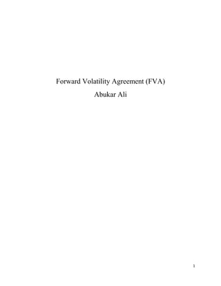
6.93%
6.90%
6.86%
6.82%
6.84%
6.86%
6.88%
6.90%
6.92%
6.94%
1m 2m 1X2

10
Table (data source Bloomberg)

11
2.1 Pricing and Hedging FVA’s
Isolating Local Volatility with “Gadgets”
Local or forward volatility is the market price of volatility you can lock in today to obtain volatility
exposure over specific some range of future times and market levels.
In the interest rate world, for example, you can lock in future interest rates between two years and
three years by going simultaneously long a three-year zero-coupon bond and short a two-year zero-
coupon bond, such that the present value of the total bond portfolio is zero.
In this way you lock in the one-year forward rate two years from now. This bond portfolio has
exposure only to this particular forward rate. As time passes, this portfolio increases in value as
the forward rate drops, and decreases as it rises.
Something similar can be done with option. A volatility gadget is a small portfolio of standard
index options, created out of a long position in a calendar spread and a short position in an
overlapping butterfly spread that has zero total options value.
This gadget is sensitive to (forward) local index volatility only in the region between the strikes
and expirations of the spreads in the gadget. Figure 3b illustrates the volatility gadget. By buying
or selling suitably constructed gadgets corresponding to different future times and index levels, we
can theoretically hedge an index option portfolio against changes in future local volatility.
See, (Derman, E., Kani, I., and Kamal, M., `Trading and Hedging Local Volatility',
QuantitativeStrategies Research Notes, Goldman Sachs & Co, 1996

12
Forward Start Straddle (STO)
Forward start option can be used to price contracts such as Forward Rate Agreement (FVA), which
is also a trade on implied volatility at a future date.
When defining a forward start, you can choose a ATM delta neutral straddle, with the strike set on
the forward start date (or strike fixing date). This is exactly the physical trade that takes place when
an FVA is fixed.
For example, you trade a delta neutral straddle forward start option with an expiry date of six
months and a forward start of three months, also known as a 3*6 FVA. In three months time, the
strike (which now has 3 months to expiry) is fixed to give a delta neutral straddle.
In this case, the buyer of the option is effectively buying volatility for three months starting in
three months. The exposure of the buyer is long 6-month Vega and short 3-month Vega. This is
quoted in the interbank market in terms of implied volatility.
The value of the forward start straddle at maturity depends then on the volatility expected in the
interval T1 to T2 and therefore it is a tool to hedge future volatility. It is sensitive to changes in
volatility but not to changes in interest rates or to a large change in spot.
Brenner, Earnest Y.Ou and Zhang have investigated the valuations of forward start options on
equity indices using Stochastic Volatility Model (SV) similar to the one by Stein and Stein (1991).
We present a summary of their key results below:
𝑑𝑆𝑡 = 𝑟𝑆𝑡 𝑑𝑡 + 𝜎𝑡 𝑆𝑡 𝑑𝐵𝑡
1
𝑑𝜎𝑡 = 𝛿(𝜃 − 𝜎𝑡)𝑑𝑡 + 𝑘𝑑𝐵𝑡
1
Where dS describes the dynamics of the underlying with a stochastic volatility.
The second equation describes the dynamics of volatility itself which is reverting to a long run
mean, and has an adjustment rate and volatility of volatility. This model assumes a zero correlation
between the conditional joint density of returns and volatility.
Results from the above model show that for relatively low strike prices, the effect of stochastic
volatility is rather small and the values are not that different from a BS value (when vol-of-vol
value is zero). For higher strike prices (OTM), the effect of vol-of-vol, is much larger.
They have also showed that the sensitivity of the straddle position to changes in initial volatility.
This shows that the position was extremely sensitive to changes in volatility and declined in value
when volatility decreased. Also, the higher the vol-of-vol, the higher is the vega of the forward
strart straddle position.

14
Trading FVA’s
An investor who believes that the implied volatility will be higher (lower) level then predicted by
the forward volatility market, can enter into a Forward Volatility Agreement (FVA):
 If implied volatility is expected to be higher ---- buy/take a long FVA position
 If implied volatility is expected to be lower ---- Sell/take a short FVA position
Figure 2.1 (3 month forward volatility from different terms-structure; source Credit Suisse
Forward volatility agreement may provide investors with long-term volatility (Vega) exposure,
without having exposure to short-term volatility (Gamma). This type of product does not have to
pay Theta as the gamma of the position is zero initially until the start of FVA’s trade date.
However, even-though the Theta may be zero for forward starting product compared to vanilla
options, if there is a rise in volatility surfaces before the forward staring period is over, they are
likely to benefit less then vanilla options (this is because the front end of the volatility surfaces
tend to move the most, and this is the area to which the forward start has no sensitivity).
While the FVA product may have zero mathematical Theta, they might suffer from the fact that
volatility and variance term-structure is usually expensive and upward sloping. The average
implied volatility of the FVA product is likely to be higher than vanilla product, which will cause
the long forward starting position to suffer carry as the volatility is re-marked lower during the
forward starting period (if a 3-month forward starting option is compared to a 3-month vanilla
option, then during the forward starting period the forward starting implied volatility should, on
average, decline.

15
GENERIC OPTION VALUATION (OVGE)
If we look at the current implied forward volatility that commences 3 month from now and expires
3 months later. We can see from the table below that the 3x6 for EURUSD quote is: 11.541%.
Even-though the market quote for future date is unknown, however, the current volatility surface
can be used to extract future or instantaneous volatilities.
We can compare the above extrapolated forward volatility from the current vanilla surface for a
given tenor to a model dependent volatility strike computed from FVA pricing.
Using Bloomberg OVGE screen, we price up 3month FVA, expiring 3 months after the FVA’s
date:
Currency Pair: EUR-USD
Trade date: 04/30/2012
FVA date: 07/30/2012
Expiry Date: 10/30/2012
Notional: 100,000,000
Not.Curncy: EUR
Agreed Vol: 11.574%
Market Quote:11.574% (3x6)
To simplify the example, we can set the agreed volatility strike the same as the market extrapolated
volatility for the tenor of FVA contract. Then;
We use the FVA template in Bloomberg OVGE screen. We enter the trade date, Domestic and
Foreign currencies, the FVA date and the final expiry of the contract. We solve for the volatility
strike that produces zero price (as close as possible). One limitation with OVGE is that it does not
have solver functionality and for this reason, we keep changing the volatility strike until we get
price that is close enough to zero or negligibly small. In this case, we have solved for 10.3%
volatility strike. The solved volatility strike gives a 0.02% price of the notional which is very small.
Please note that in order to speed up the calculations; we are using MC Heston but only up to 1000
sample paths.

16
As expected when using stochastic volatility models, the model tends to undervalue the market
price or quoted prices and this is mainly due to the correlation between spot and volatility. The
dynamics of the observed volatility surface when spot moves is inconsistent with the result from
stochastic volatility models.
To hedge the above FVA contract:
Enter long 6 month EUR-USD Straddle position on EUR 10,000,000 notional
Enter short 3 month EUR-USD Straddle position on EUR 10,000,000 notional
The net position should leave us a long 3 month long Vega. On the trade date, the position should
have zero Delta and Gamma but we with constant Vega as spot moves from trade date until the
contract (FVA’s) start date.
We can maintain constant Vega until the FVA date but once the FVA date is reached, the position
will have regular Vega position as Vanilla option and will need to be risk managed. As the market
moves, the strike is then away from the DNS (Delta-Neutral Straddle). To maintain the Delta
neutrality of the position, the trader needs to buy/sell the underlying.
As mentioned above the FVA contract does not need to be delta hedged before the forward starting
period ends. However, such contracts need to be Vega hedged with vanilla, out-of-the money
Straddles (as they do have zero Delta and Gamma). A long OTM straddle has to be purchased on
the expiry date of the option (6 month), while a short OTM Straddle has to be sold on the strike
fixing date (3 month). As the spot moves, the delta of these Straddles is likely to move away from
zero, requiring re-hedging of the position, which increases the costs (which are likely to be passed
on to clients) and risks (unknown future volatility and skew) to the trader.
From inception of the contract until the FVA’s date, we maintain a constant Vega position. Given
the above portfolio of vanilla positions, we then risk manage the Delta/Gamma risk, Vega risk, as
well as Vanna and Volga risk.

17
DELTA RISK:
𝐶𝑎𝑙𝑙𝑂𝑝𝑡𝑖𝑜𝑛 = 𝑆 𝑥𝑁(𝑑1) − 𝐾𝑒−𝑟𝑇
𝑁(𝑑2)
𝑃𝑢𝑡𝑂𝑝𝑡𝑖𝑜𝑛 = −𝑆 𝑥𝑁(−𝑑1) + 𝐾𝑒−𝑟𝑇
𝑁(𝑑2)
Where 𝑑1 =
𝑙𝑛(
𝑆
𝐾
)+(𝑟+
𝜎2
2
)𝑇
𝜎√𝑇
Delta = N(d1)
To maintain the delta neutrality of the position once after the FVA’s date, we need to buy/sell an
amount equivalent of the delta of the position.
STRIKE-LESS VEGA
Both Volatility Swap and FVA’s initially give exposure to strike-less Vega (exposure to implied
volatility that remains constant as spot moves). This is because the ATM straddle is not set until
the FVA’s fixing date / start date.
The FVA’s strike-less Vega is constant until the strike fixing date and once the strike is fixed at
fixing date of the FVA, the Vega profile is similar to Vanilla and varies with the underlying.
RISK MANAGE GAMMA OF VOLATILITY EXPOSURE (VOLGA)
Volga represents the sensitivity of vega to change in implied volatility. Mathematically;
𝑉𝑜𝑙𝑔𝑎 =
δ2
P
σδ2
 The first derivative of vega with respect to a change in volatility.

18
 The second derivative of option value with respect to a change in volatility (hence
the other name as Gamma Vega).
The volga is also referred to as Vomma. For volatility movements, Volga is to Vega what gamma
is to delta (for spot movement).
For complex exotics such as FVA’s that requires stochastic volatility models, one need to compute
volga and other Greeks with respect to model parameters.
The interest of Volga is to measure the convexity of an FVA position with respect to volatility.
FVA contract with high Volga benefits from volatility of volatility.
Hence, volatility dependent derivatives such as FVA with substantial Volga, pricing with a
stochastic volatility model with high volatility of volatility may change the price dramatically.
For complex exotics such as FVA, traders cannot just simply ignore the risk due to the change of
Vega. They have to understand the change of the Vega with respect to the spot (see Vanna) and to
the volatility itself. And to have a better understanding of Volga, it is important to stress the variety
of models to account for the smile surface. In particular the shape of Volga would crucially depend
on the choice of model out of the following list of models:
 Stochastic volatility models: the correlation effect between the stock and the volatility
plays an important role in shaping the vega change.
 Local volatility model where the resulting local volatility is a function of the
underlying itself.
 Jumps models with jumps correlated to the volatility parameters.
 Combination of the above, like Lévy processes.

19
 Discrete type option pricing models that are in fact, discretised versions of the models
above. For instance ARCH/GARCH processes are just discrete versions of stochastic
volatility models.
RISK MANAGE SKEW EXPOSURE (VANNA)
Vanna measures the change in delta due to a change in volatility. It measures the size of the skew
position. Vanna is the slope of vega plotted against spot.
The Vanna is a second order “cross” Greeks. Like any other cross Greeks, the Vanna can be
defined in many ways:
 First derivative of Vega with respect to a change in the underlying.
 First derivative of delta with respect to a change in volatility.
 Second derivative of option value with respect to a joint moved in volatility and underlying.
To account for the complexity of the smile and in particular its skew and convexity, one needs to
take the route of more realistic models including deterministic local volatility, stochastic volatility
and jumps (see smile modeling), and most recent model that combines both Local Volatility and
Stochastic Volatility models (SLV).
Stochastic models can change considerably the shape of the Vanna as they explicitly specify the
correlation between volatility and the spot. If spot and volatility are positively correlated, the
holder of the option with positive Vanna will benefit from the correlation.

20
Review of Variance Swap risks:
To hedge variance swap, market makers hold a portfolio of single stock options and carry out
daily delta hedging.
The hedge held by market-makers consisted of a portfolio of options built in such a way to have
constant dollar gamma both for movements in the stock prices and for the passage of time. This
portfolio can be theoretically created by combining an infinite number of options with strikes
spanning all possible values of the stock and the same maturity as the variance swap. Figure 3
shows the dollar gamma profile of individual options of different strikes. Weighting the options
according to 1/Strike*Strike creates a portfolio with the flat gamma profile needed to hedge a
variance swap
The static hedge has some practical limits:
1- Impossible to trade an infinite number of options with infinite number of strikes
2- Liquidity of OTM options are limited, restricting the number of tradable options
3- Market makers are unable to buy complete theoretical hedge
4- We can only do approximate hedge within specified range of spot
Figure 4 shows the dollar gamma profile of holding portfolios of 1, 2 and 5 options, and illustrates
the limited range of spot levels for which the dollar gamma profile is flat.
Most brokers thought that the restricted portfolio was a good hedging solution for replicating
variance swaps, as it was cheap and easy to trade, and neutralized their risks for a wide range of
stock prices, encompassing all but the most extreme scenarios. However, the 2008 crisis led to
large drops in single stock prices, and many market makers found themselves unhedged in the new
trading range
After the market declined, many single stock option desks became forced buyers of low strike
options, in order to manage the gamma and vega risk of the variance swap positions in their books.
In fact, by selling variance swaps, the traders had committed to deliver the P/L of a constant dollar

21
gamma portfolio, irrespective of the spot level, but their replicating portfolio did not have
sufficient dollar gamma at the new spot levels. Market makers were therefore forced to buy low
strike options at the post-crash volatility level, which was much higher than the one prevailing
when they sold the variance swap, and therefore incurred heavy losses.
Not re-hedging the gamma risk was not a possibility, as this would have left the books exposed to
potentially catastrophic losses if the stock prices declined further, and volatility continued to
increase. The convexity of the variance swap payoff further exacerbated the downside risk. This
situation led to large losses for many market-makers in the single stock variance swap markets. In
turn this led banks to re-assess the risk of making markets in these instruments and to a substantial
shutdown of the single stock variance swap market

22
Review of Volatility Swap risks:
Delta-hedging options leads to a P/L linked to the variance of returns rather than volatility. To
achieve the linear exposure to volatility which volatility swaps provide it is therefore necessary to
dynamically trade in portfolios of options, which would otherwise provide an exposure to the
square of volatility. A volatility swap can be thought as a non-linear derivative of realized variance,
the ‘underlier’ that can be traded through portfolios of delta-hedged options.
To hedge volatility swap with variance swap, the trader would need to trade in and out of variance
swaps in order to replicate the square root of variance payoff of the volatility swap.
The volatility swap payoff can be locally approximated by a variance swap, where the variance
swap begins to outperform the further realized volatility moves from the initial strike. Thus, the
volatility swap could theoretically be replicated through “delta-hedging” by trading dynamically
in the variance swap, where the “delta” is the sensitivity to the instruments’ underlying, namely
realized variance. Changes in this volatility “delta” will depend on the investor’s estimate of
volatility of volatility.
A volatility swap can be replicated using a delta-hedged portfolio of options, where the portfolio
of options is dynamically rebalanced to replicate the Vega and gamma profile of the volatility swap
across the range of spot prices.
One possible approach to hedging the volatility swap is to trade delta-hedged ratio strangles (e.g.
short 1.5 80% strike puts and short one 120% call to hedge a long volatility swap), where the ratio
and strikes are set in order to minimize the net exposure to volatility across the skew (i.e. to attempt
to match the Vega profile of the options to the volatility swap over a range of anticipated spot
levels). Since the Vega exposure of the strangle and volatility swap differ as the spot changes, the
strangles will have to be re-striked when the net exposure to volatility exceeds the trader’s
tolerance.

23
Below, we can see how the Vega and gamma sensitivity of the volatility swap compares to a
sample ratio strangle chosen to minimize the error for near-the-money Vega exposure for an
assumed level of volatility and skew.
The strangle notionals, strikes and the ratio of puts to calls will depend on the shape of the implied
volatility skew at the time the hedge is put in place.
Additionally, it may not be possible to simultaneously replicate both vega and gamma well over a
broad range of spot levels with this approach, as is the case in the example below where the chosen
portfolio poorly replicates the gamma exposure of the volatility swap below the spot.
- Re-striking may cause the need for new strangles to be initiated with significant different
volatility if the volatility level has shifted.
- More transaction costs
- P&L risk when re-striking the hedging portfolio will depend on vol-of-vol
- Higher vol-of-vol leads to largest shifts in pricing the options used for the hedge

24
Valuation Models:
Volatility swaps and forward volatility agreements are more complex instrument to price.
Volatility is the square root of variance, and is a more complex derivative of variance. Its value
depends not just on volatility, but on the volatility of volatility, and you have to dynamically hedge
it by trading variance swaps as the underlier. This is possible too, but needs a model for the
volatility of volatility.
We will review existing models and the most appropriate model for valuation of Forward Volatility
Agreement contract. However, the selected model should be able to produce realistic hedge ratios
or Greeks such as Delta, Gamma, Vega, as well as vega risk with respect to changes in both spot
and implied volatility.
3.1 Appropriate Models;
LOCAL VOLATILITY MODEL (LV)
The Local Volatility Model (LV) extends the Black-Scholes model by allowing the instantaneous
volatility to depend on spot and time (Dupire 1994).
𝑑𝑆 = 𝑆𝑡(𝑟𝑡 − 𝑞𝑡) + 𝜎(𝑡, 𝑆𝑡)𝑆𝑡 𝑑𝑊 (3.1)
The Local Volatility function 𝜎(𝑡, 𝑆𝑡) is a function to be inserted into the (3.1) which will
reproduce the current vanilla market prices. The function has no stochasticity of its own, just
deterministic state dependency on time and underlying. This model class is considered less
complex since it does not involve individual stochastic differential equations (SDE) for the
volatility, it is merely described by a function.
Dupire found that the Local Volatility (LV) function could be derived as:
𝜎(𝐾, 𝑇) = √2
𝛿𝐶
𝛿𝐾
+ (𝑟 − 𝑑)𝐾
𝛿𝐶
𝛿𝐾
+ 𝑑𝐶
𝐾2 𝛿2 𝐶
𝛿𝐾2
 Simplest model consistent with the market
 Local volatilities are forward volatilities
 Arbitrage free (positive and regular)
 Implied volatilities surface with strike extrapolation provides variance swap fair value

25
 Good IV surface should give an accurate risk neutral density
The deterministic LV function, represents a market consensus estimates for the instantaneous
volatility at some future time t with the asset at value S. It can be shown that the local variance
𝜎2
(𝑆, 𝑡) is the expectation of the future instantaneous variance 𝜎2
(𝑡) at time t conditional on the
asset having a value S at time t.
Known Issues using Local Volatility (LV) Model
Since in local volatility models the volatility is a deterministic function of the random underlying
price, local volatility models are not very well used to price cliquet options, forward starting
options, Forward Volatility Agreement, as well as variance and volatility swaps, whose values
depend specifically on the random nature of volatility itself
Lian (2010) noted that one of the problems related to applying the Dupire equation is that options
might not be available for a complete range of strikes and maturity.
With insufficient data, the LV function might be severely misspecified. In addition, strikes for
deep ITM and OTM might cause the fraction in the above equation to become extremely small
which could lead to numerical issues as addressed in Lian (2010).
Local volatility Models are easy to implement and theoretically self consistent, as it is possible to
perfectly replicate all the vanilla option prices and to hedge every product with vanilla options.
However, Hagen (2002) argues that the dynamic behavior of spot volatility smile and skew
predicted by local volatility models is exactly opposite to the behavior observed in the market
place:
When the prices decreases, Local Volatility Models predict that the smile shifts to higher prices.
When the price increases, Local Volatility Models predict that the smile shifts to lower prices. In
reality asset prices and market smiles moves in the same direction. These inconsistencies lead to
incorrect hedges and hence incorrect pricing for exotic options.
Implied volatility 𝜎(𝐾, 𝑓) if the forward prices decreases from f0 to f (solid line).
Implied volatility 𝜎(𝐾, 𝑓) if the forward prices increases from f0 to f (solid line).

26
Local volatility models are deterministic models and produce sharply flattened future volatility
smiles and skews as seen in figure below, which shows the three month forward implied volatility
skew at different reset dates, where 0M refers to the vanilla three-month option and 60M refers to
an option with three months' expiry starting in five years' time. We can see as we go out further in
time that the volatility skew and curvature decays. This behavior is not observed in the market.
Notice the flattening of the surface for lower and higher strikes Local Volatility surface for SX5E index
There are no documented empirical research testing the pricing result of FVA’s against the market,
however, Behvan (2010) investigated the pricing of structures that depend on forward volatility
such as Cliquet options (strip of forward starting options). Behvan (2010) compares the pricing
result of Cliquet using Local Volatility model against market consensus (Totem).
Red indicates results from the Local Vol. Model which are outside of the market consensus.

27
STOCHASTIC VOLATILITY MODELS
(HESTON);
The first stochastic volatility model was proposed by Heston in 1993, who introduced an intuitive
extension of the well known Black and Scholes modelization. He assumed that the spot price
follows the diffusion: that is, a process resembling geometric Brownian motion with a non-
constant instantaneous variance V (t). Furthermore, he proposed that the variance is a CIR process,
that is a mean reverting stochastic process of the form:
𝑑𝑆𝑡 = (𝑟𝑑 − 𝑟𝑓)𝑆𝑡 𝑑𝑡 + √𝑉𝑡 𝑆𝑡 𝑑𝑊𝑡
1
𝑑𝑉𝑡 = 𝑘(𝜃 − 𝑉𝑡)𝑑𝑡 + 𝜎√𝑉𝑡 𝑑𝑊𝑡
2
And the two Brownian motions are correlated with each other:
1. Initial volatility:"V(0), Not directly observable
2. Long term variance: 𝜽
3. Speed of mean reversion of volatility: k
4. Volatility of volatility: 𝝈
5. Correlation between spot exchange rate and volatility: 𝝆
All these parameters can be calibrated.
We can interpret the parameters 𝝈 and 𝝆 as being responsible for the skew, the volatility of
variance controlling the curvature and the correlation the tilt.
The other three parameters (V(0), 𝜽, and k) control the term structure of the model; where the mean
reversion controls the skewness of the curve from the short volatility level to the long volatility
level.
The Heston model is a generalization of the Black-Scholes model. Taking the limits 𝝈--> 0, and
k  0, we recover the Black-Scholes PDE with constant volatility.
The volatility-of-volatility and mean reversion have opposite effect on the dispersion of volatility.
Volatility-of-volatility allows a large variation of future values of volatility; Mean-reversion
reversion tends to push future values of volatility towards the long-term value of volatility.

28
Advantages:
The model intuitively extends the Black and Scholes model, including it as a special case. The
model is better used to price derivatives whose underlying is the spot itself, as it directly models
St. Heston’s setting take into account non-lognormal distribution of the assets returns, leverage
effect, important mean-reverting property of volatility and it remains analytically tractable.
Limitations:
Empirical evidence suggests that Stochastic Volatility model (SV) is able to capture the empirical
surface quite well in general. However as noted in many research papers the model does a rather
poor job fitting the smile at short maturities. See figure below.
The model has five parameters to calibrate. The volatility does not depend on the level of the spot,
which may a drawback when the model is used to price products sensitive with respect to the spot
of the underlying.
The dynamics of the calibrated Heston Model predict that:
- Volatility can reach zero
- Stay at zero for some time
- Volatility is likely to stay extremely low or very high for long periods of time
Bloomberg have implemented Heston model for pricing FX options and find similar weaknesses
mentioned above – the model’s inability to generate the smirks and the smiles for short options.
This is a characteristic for all stochastic volatility models.
Below we list the three main problems reported in the Bloomberg study:
 Heston model cannot fit a general volatility surface, which may contain 20-30 data
points.
 Over short horizons, the Heston model does not generate the amount of skew and
curvatures quoted in actual volatility surfaces. ( This short comings of stochastic volatility
models can be alleviated by adding jump component to the model)
 The time dependency in implied volatilities of ATM options is not in general of the form
of an exponential transition from short-term to long-term levels as prescribed by the form
of mean-reversion of the Heston model Parameter effects on the implied volatility smile
in the Heston SV model.

29
Under the Bloomberg study, a set of Heston model parameters are calibrated using EUR/JPY,
EUR/USD, GBP/USD and USD/JPY and their volatility surfaces. The relative error of volatility
implied by the Heston option pricingi model and the input implied volatility. The test is based on
ATM, 25 and 10-delta points with expiries of 1 week, 1 month, 6 month and 1 year.
Errors are smaller for the 25-delta options but the error increases for 10-delta options. For 1
week and 1 month options, the fit is not very good as expected for the Heston model. Errors are
around 5-10% for all delta values.

30
Below is a list of pros and cons of stochastic volatility models compiled by Peter Carr and Roger
Lee in their joint presentation; Robust Replciation of Volatility Derivatives, April 2003, Stanford
University.
 All of the literature on volatility derivatives employs some kind of stochastic volatility
(SV) model.
 Furthermore, the models typically (but not always) assume that the price process and the
volatility process are both continuous over time.
 To the extent that these assumptions are correct and that the particular process specification
is correct, one can use dynamic trading in one option and its underlying to hedge.
 Most of the SV models used further assume that prices and instantaneous volatility both
diffuse leading to a simple and parsimonious world view. However, simple SV models
cannot simultaneously fit option prices at long and short maturities. Furthermore, since
instantaneous volatility is not directly observable, the assumption that the diffusion
coefficients of the volatility process are known is debatable.
 Indeed, the SV diffusion parameters implied from time series typically differ from the risk-
neutral parameters, contradicting the implications of Girsanov’s theorem.
 Complicating the pricing and hedging of volatility derivatives is the ugly fact that prices
jump.
 Furthermore, when prices jump by a large amount, it is widely believed that expectations
of future realized volatility jump as well. The high levels of mean reversion and vol-of-vol
implied from option prices further suggests that volatility jumps.
 When price and/or volatility can jump from one level to any other, then in a model with
two or more sources of uncertainty, perfect replication typically requires dynamic trading
in a portfolio of options.
 While option bid/ask spreads typically render this strategy as prohibitively expensive at
the individual contract level, knowledge of desired option hedges can be enacted at the
aggregate portfolio level.
 Can we use dynamic trading in a portfolio of options to develop a theory which does not
require a complete specification of the stochastic process for volatility?
DETERMISTIC AND STOCHASTIC VOLATILITY MODELS: REULTS

31
First, the valuation and hedging of volatility swap as well as forward volatility agreements are
more complicated then Variance swap contracts. The standard deviation is the square root of the
variance; but the square root is a non linear function. It is this linearity that makes the replication
and valuation of volatility based swaps more complex. Oliver Brockhaus and Douglas Long (Risk,
Jan. 2000), investigated the pricing of volatility derivatives and used both deterministic and
stochastic volatility based model.
According to the above authors, a comparison between a deterministic volatility model (DVM)
and stochastic volatility model (SVM) shows that the price of DVM is always higher. As can be
seen from the figure below, the price difference increases with decreasing absolute asset-volatility
correlation and increasing volatility of volatility.
A model-independent approach can be derived for volatility swap using Taylor expansion of the
square root function around some value that is close to the expected volatility swap value. So in
approximating volatility swaps only to 1st
order, we do not capture the effects of stochastic
volatility (volatility convexity).
1st
and 2nd
order approximation for the volatility swap. model dependency of volatility swap.
So, the 1st
and 2nd
order Taylor expansions provide two approximations that respectively
overestimate and underestimate the true value of the swap. Since Forward volatility agreement
requires the square root of the variance, one can argue that we might expect similar results too.
STOCHASTIC LOCAL VOLATILITY MODEL (SLV);
 Classical models such as local volatility (LV) and stochastic volatility (SV) are in fact calibrated to
and completely determined by the vanilla market
 They offer no extra flexibility in matching the market dynamics.

32
 In the FX market, stochastic volatility (SV) behaves better than local volatility (LV) from a
dynamics point of view,
 But Stochastic Volatility (SV) fails to calibrate to the vanillas prices
 Mixing the two seems to be the answer and most market participants have moved in that
direction.
Because of the limitations of the Local and Stochastic models on their own, recently the market
practitioners have settled on using a model that combines both of the above models called
Stochastic Local Volatility model (SLV).
At the moment there is not much empirical tests on valuations of volatility derivatives (products)
using this new approach, however, implementation and tests on barrier type exotics show:
- calibration matches the entire volatility surface to the very distant wings
- better model generated prices for reverse KO, Touches and Digital
- consistent with market dynamics.
For valuation of FVA, it would require a model that has the above features. It will also require not
only better calibration but the calibrated volatility surface should have correct dynamics.
To test the SLV model, we would need to generate list of FVA prices for a given maturity using
various mixing fractions. We can then compare these prices with market quoted prices (provided
there are liquid OTC prices). For more detailed discussion on the implementations and empirical
result on SLV model, see Tataru and Fisher, (2010).
Bloomberg SLV Model
The SLV model that we investigate is described by:

33
dtdWdW
dWVvvoldtVkdV
dWVtSLdtrr
S
dS
tt
tttt
tttfd
t
t

 



21
2
1
)(
),()(
),( tSL t = Local Volatility, K = speed of mean reversion, Θ= mean reversion level, Vvol
=volatility of variance, Ρ =correlation.
The mixing of LV and SV features is controlled mostly by vvol, followed as importance by the
correlation ρ. For SLV to degenerate to a pure LV model one would set vvol=0 and to obtain a
pure SV model one would set ),( tSL t =1.
Calibration:
1. Find the stochastic parameters to match the market dynamics
2. And then calibrate the local vol. function ),( tSL t to match the vanilla market
calibrate
to match the vanilla market
“A rigorous approach to finding the stochastic parameters rests on a quantification of the market
dynamics. This can be represented by SpotATM/ and SpotRR/ or other ways to quantify the
movements of the implied volatility surface given a move in spot.”
References
Grigore Tataru, Travis Fisher, Quantitative Development Group, Bloomberg “Stochastic Local Volatility”
(February, 2010).
GIVEN
K, theta,
Vvol, p
),( tSL t
Local
Volatility
Vanilla
Market
prices

34
Patrick Hagan, Deep Kumar, Andrew S. Lesniewski and Diana E. Woodward. Managing smile risk.
Wilmott Magazine, pages 86-108, July 2002.
Steven L. Heston. A closed-form solution for options with stochastic volatility with applications to bond
and currency options. Review of Financial Studies, 6(2):327{343, 1993.
Guanghua Lian. Pricing volatility derivatives with stochastic volatility. PhD thesis, University
of Wollongong, 2010.
Iddo Yekutieli. Implementation of Heston Model for the Pricing of GX Options. Bloomberg LP. Bloomberg
Financial Markets (BFM), June 22 2004.
Collin Bennet, Miguel A.Gil. “Volatility Trading – Trading volatility, correlation, termstructure and skew.
Equity Derivatives. Santander, Global Banking and Markets.
Menachem Brenner, Ernest Y. Ou, Jin E Zhang. “ Hedging Volatility Risk”. Journal of Banking and Finance
30 (2006) 811 – 821
Carr, P., and L. Wu (2007). .Stochastic Skew in Currency Options,. Journal of Financial Economics, 86,
213.247.
Jiang, G.J., and Y.S. Tian (2005). .The Model-Free Implied Volatility and Its Information Content,. Review
of Financial Studies 18, 1305.1342.

FVA

Empfohlen

Empfohlen

Weitere ähnliche Inhalte

Was ist angesagt?

Was ist angesagt? (20)

Ähnlich wie FVA

Ähnlich wie FVA (20)

FVA