Biofluid Chapter 3.6.pdf

For each generation rate, the minimum value of h needed to maintain Ts,2 350 C
may be determined from the figure.
3. The temperature distribution, Equation 7, may also be obtained by using the results of
Appendix C. Applying a surface energy balance at r r1, with q(r)
may be determined from Equation C.8 and the result substituted into Equa-
tion C.2 to eliminate Ts,1 and obtain the desired expression.
3.6 Heat Transfer from Extended Surfaces
The term extended surface is commonly used to depict an important special case involving
heat transfer by conduction within a solid and heat transfer by convection (and/or radiation)
from the boundaries of the solid. Until now, we have considered heat transfer from the
boundaries of a solid to be in the same direction as heat transfer by conduction in the solid.
In contrast, for an extended surface, the direction of heat transfer from the boundaries is
perpendicular to the principal direction of heat transfer in the solid.
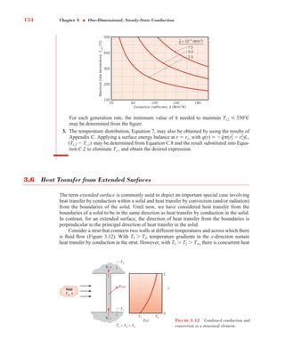
Consider a strut that connects two walls at different temperatures and across which there
is fluid flow (Figure 3.12). With T1 T2, temperature gradients in the x-direction sustain
heat transfer by conduction in the strut. However, with T1 T2 T앝, there is concurrent heat
(Ts,2 Ts,1)
q̇␲(r2
2 r2
1)L,
Maximum
tube
temperature,
T
s,2
(°C)
500
400
300
200
100
20
Convection coefficient, h (W/m2•K)
60 100 140 180
7.5
q
•
× 10–6
(W/m3
)
5.0
2.5
154 Chapter 3 䊏 One-Dimensional, Steady-State Conduction
FIGURE 3.12 Combined conduction and
convection in a structural element.
x
L
qconv
qx, 1
qx, 2
T1
0
T2
T1
T(x)
T1 T2 T∞
T2
Fluid
T∞, h
CH003.qxd 2/24/11 12:25 PM Page 154

transfer by convection to the fluid, causing qx, and hence the magnitude of the temperature
gradient, 兩dT/dx兩, to decrease with increasing x.
Although there are many different situations that involve such combined conduction–
convection effects, the most frequent application is one in which an extended surface is
used specifically to enhance heat transfer between a solid and an adjoining fluid. Such an
extended surface is termed a fin
Consider the plane wall of Figure 3.13a . If Ts is fixed, there are two ways in which the
heat transfer rate may be increased. The convection coefficient h could be increased by
increasing the fluid velocity, and/or the fluid temperature T앝 could be reduced. However,
there are many situations for which increasing h to the maximum possible value is either
insufficient to obtain the desired heat transfer rate or the associated costs are prohibitive.
Such costs are related to the blower or pump power requirements needed to increase h
through increased fluid motion. Moreover, the second option of reducing T앝 is often
impractical. Examining Figure 3.13b , however, we see that there exists a third option. That
is, the heat transfer rate may be increased by increasing the surface area across which the
convection occurs. This may be done by employing fin that extend from the wall into
the surrounding fluid. The thermal conductivity of the fin material can have a strong effect
on the temperature distribution along the fin and therefore influences the degree to which
the heat transfer rate is enhanced. Ideally, the fin material should have a large thermal con-
ductivity to minimize temperature variations from its base to its tip. In the limit of infinite
thermal conductivity, the entire fin would be at the temperature of the base surface, thereby
providing the maximum possible heat transfer enhancement.
Examples of fin applications are easy to find. Consider the arrangement for cooling
engine heads on motorcycles and lawn mowers or for cooling electric power transformers.
Consider also the tubes with attached fins used to promote heat exchange between air and
the working fluid of an air conditioner. Two common finned-tube arrangements are shown
in Figure 3.14.
Different fin configurations are illustrated in Figure 3.15. A straight fi is any extended
surface that is attached to a plane wall. It may be of uniform cross-sectional area, or its
cross-sectional area may vary with the distance x from the wall. An annular fi is one that is
circumferentially attached to a cylinder, and its cross section varies with radius from the
wall of the cylinder. The foregoing fin types have rectangular cross sections, whose area
may be expressed as a product of the fin thickness t and the width w for straight fins or the
circumference 2␲r for annular fins. In contrast a pin fin or spine, is an extended surface of
circular cross section. Pin fins may also be of uniform or nonuniform cross section. In any
FIGURE 3.13 Use of fins to enhance
heat transfer from a plane wall.
(a) Bare surface. (b) Finned surface.
q = hA(Ts – T∞)
T∞, h
T∞, h
A
Ts
Ts, A
(a) (b)
3.6 䊏 Heat Transfer from Extended Surfaces 155
CH003.qxd 2/24/11 12:25 PM Page 155

application, selection of a particular fin configuration may depend on space, weight, manufac-
turing, and cost considerations, as well as on the extent to which the fins reduce the surface
convection coefficient and increase the pressure drop associated with flow over the fins.
3.6.1 A General Conduction Analysis
As engineers we are primarily interested in knowing the extent to which particular
extended surfaces or fin arrangements could improve heat transfer from a surface to the
surrounding fluid. To determine the heat transfer rate associated with a fin, we must first
obtain the temperature distribution along the fin. As we have done for previous systems, we
begin by performing an energy balance on an appropriate differential element. Consider
the extended surface of Figure 3.16. The analysis is simplified if certain assumptions are
made. We choose to assume one-dimensional conditions in the longitudinal (x-) direction,
even though conduction within the fin is actually two-dimensional. The rate at which
energy is convected to the fluid from any point on the fin surface must be balanced by
the net rate at which energy reaches that point due to conduction in the transverse (y-, z-)
direction. However, in practice the fin is thin, and temperature changes in the transverse
FIGURE 3.14 Schematic of typical finned-tube heat exchangers.
FIGURE 3.15 Fin configurations. (a) Straight fin of uniform cross section. (b) Straight fin of
nonuniform cross section. (c) Annular fin. (d) Pin fin.
Liquid
flow
Gas
flow
Gas flow
Liquid flow
r
x x x
t
w
(a) (b) (c) (d)
CH003.qxd 2/24/11 12:25 PM Page 156

direction within the fin are small compared with the temperature difference between the fin
and the environment. Hence, we may assume that the temperature is uniform across the
fin thickness, that is, it is only a function of x. We will consider steady-state conditions and
also assume that the thermal conductivity is constant, that radiation from the surface is neg-
ligible, that heat generation effects are absent, and that the convection heat transfer coeffi-
cient h is uniform over the surface.
Applying the conservation of energy requirement, Equation 1.12c, to the differential
element of Figure 3.16, we obtain
(3.61)
From Fourier’s law we know that
(3.62)
where Ac is the cross-sectional area, which may vary with x. Since the conduction heat rate
at x dx may be expressed as
(3.63)
it follows that
(3.64)
The convection heat transfer rate may be expressed as
(3.65)
where dAs is the surface area of the differential element. Substituting the foregoing rate
equations into the energy balance, Equation 3.61, we obtain
d
dx 冢Ac
dT
dx冣 h
k
dAs
dx
(T T앝) 0
dqconv hdAs(T T )
qxdx kAc
dT
dx
k d
dx 冢Ac
dT
dx冣dx
qxdx qx
dqx
dx
dx
qx kAc
dT
dx
qx qxdx dqconv
FIGURE 3.16 Energy balance for an
extended surface.
qx+dx
dqconv
Ac(x)
dAs
qx
dx
z
x
y
x
CH003.qxd 2/24/11 12:25 PM Page 157

or
(3.66)
This result provides a general form of the energy equation for an extended surface. Its solu-
tion for appropriate boundary conditions provides the temperature distribution, which may
be used with Equation 3.62 to calculate the conduction rate at any x.
3.6.2 Fins of Uniform Cross-Sectional Area
To solve Equation 3.66 it is necessary to be more specific about the geometry. We begin with
the simplest case of straight rectangular and pin fins of uniform cross section (Figure 3.17).
Each fin is attached to a base surface of temperature T(0) Tb and extends into a fluid of
temperature T앝.
For the prescribed fins, Ac is a constant and As Px, where As is the surface area mea-
sured from the base to x and P is the fin perimeter. Accordingly, with dAc /dx 0 and
dAs /dx P, Equation 3.66 reduces to
(3.67)
To simplify the form of this equation, we transform the dependent variable by defining an
excess temperature ␪ as
(3.68)
where, since T앝 is a constant, d␪/dx dT/dx. Substituting Equation 3.68 into Equation 3.67,
we then obtain
(3.69)
d2
␪
dx2
m2
␪ 0
␪(x) ⬅ T(x) T앝
d2
T
dx2
hP
kAc
(T T앝) 0
d2
T
dx2
冢1
Ac
dAc
dx 冣dT
dx
冢1
Ac
h
k
dAs
dx 冣(T T ) 0
FIGURE 3.17 Straight fins of uniform cross section. (a) Rectangular
fin. (b) Pin fin.
qf
T∞, h
T∞, h
x
L
Ac
D
qconv
P = D
Ac = D2
/4
π
L
x
qf
Tb
w
t
qconv
Ac
P = 2w + 2t
Ac = wt
(a) (b)
Tb
π
CH003.qxd 2/24/11 12:25 PM Page 158

where
(3.70)
Equation 3.69 is a linear, homogeneous, second-order differential equation with constant
coefficients. Its general solution is of the form
(3.71)
By substitution it may readily be verified that Equation 3.71 is indeed a solution to
Equation 3.69.
To evaluate the constants C1 and C2 of Equation 3.71, it is necessary to specify appropriate
boundary conditions. One such condition may be specified in terms of the temperature at the
base of the fin (x 0)
(3.72)
The second condition, specified at the fin tip (x L), may correspond to one of four differ-
ent physical situations.
The first condition, Case A, considers convection heat transfer from the fin tip. Apply-
ing an energy balance to a control surface about this tip (Figure 3.18), we obtain
or
(3.73)
That is, the rate at which energy is transferred to the fluid by convection from the tip must
equal the rate at which energy reaches the tip by conduction through the fin. Substituting
Equation 3.71 into Equations 3.72 and 3.73, we obtain, respectively,
(3.74)
and
Solving for C1 and C2, it may be shown, after some manipulation, that
(3.75)
The form of this temperature distribution is shown schematically in Figure 3.18. Note that
the magnitude of the temperature gradient decreases with increasing x. This trend is a con-
sequence of the reduction in the conduction heat transfer qx(x) with increasing x due to
continuous convection losses from the fin surface.
We are particularly interested in the amount of heat transferred from the entire fin.
From Figure 3.18, it is evident that the fin heat transfer rate qf may be evaluated in two
␪
␪b

cosh m(L x) (h/mk) sinh m(L x)
cosh mL (h/mk) sinh mL
h(C1emL
C2emL
) km(C2emL
C1emL
)
␪b C1 C2
h␪(L) k
d␪
dx
冏xL
hAc[T(L) T앝] kAc
dT
dx
冏xL
␪(0) Tb T앝 ⬅ ␪b
␪(x) C1emx
C2emx
m2
⬅ hP
kAc
CH003.qxd 2/24/11 12:25 PM Page 159

alternative ways, both of which involve use of the temperature distribution. The simpler
procedure, and the one that we will use, involves applying Fourier’s law at the fin base.
That is,
(3.76)
Hence, knowing the temperature distribution, ␪(x), qf may be evaluated, giving
(3.77)
However, conservation of energy dictates that the rate at which heat is transferred by con-
vection from the fin must equal the rate at which it is conducted through the base of the fin.
Accordingly, the alternative formulation for qf is
(3.78)
where Af is the total, including the tip, fin
surface area. Substitution of Equation 3.75 into
Equation 3.78 would yield Equation 3.77.
The second tip condition, Case B, corresponds to the assumption that the convective
heat loss from the fin tip is negligible, in which case the tip may be treated as adiabatic and
(3.79)
Substituting from Equation 3.71 and dividing by m, we then obtain
C1emL
C2emL
0
d␪
dx
冏xL
0
qf 冕Af
h␪(x) dAs
qf 冕Af
h[T(x) T ] dAs
qf 兹hPkAc␪b
sinh mL (h/mk) cosh mL
qf qb kAc
dT
dx
冏x0
kAc
d␪
dx
冏x0
qb = qf hAc[T(L) – T∞]
Tb
–kAc
dT
__
dx x=L
qconv
Fluid, T∞
b
θ
0
0 L
x
(
x
)
θ
FIGURE 3.18 Conduction and
convection in a fin of uniform
cross section.
CH003.qxd 2/24/11 12:26 PM Page 160

Using this expression with Equation 3.74 to solve for C1 and C2 and substituting the results
into Equation 3.71, we obtain
(3.80)
Using this temperature distribution with Equation 3.76, the fin heat transfer rate is then
(3.81)
In the same manner, we can obtain the fin temperature distribution and heat transfer rate
for Case C, where the temperature is prescribed at the fin tip. That is, the second boundary con-
dition is ␪(L) ␪L, and the resulting expressions are of the form
(3.82)
(3.83)
The very long fin Case D, is an interesting extension of these results. In particular, as L l 앝,
␪L l 0 and it is easily verified that
(3.84)
(3.85)
The foregoing results are summarized in Table 3.4. A table of hyperbolic functions is provided
in Appendix B.1.
qf 兹hPkAc␪b
␪
␪b
emx
qf 兹hPkAc␪b
cosh mL ␪L /␪b
sinh mL
␪
␪b

(␪L/␪b) sinh mx sinh m(L x)
sinh mL
qf 兹hPkAc␪b tanh mL
␪
␪b

cosh m(L x)
cosh mL
TABLE 3.4 Temperature distribution and heat loss for fins of uniform cross section
Tip Condition Temperature Fin Heat
Case (x ⴝ L) Distribution ␪/␪b Transfer Rate qƒ
A Convection heat
transfer:
h␪(L) kd␪/dx冨x⫽L
(3.75) (3.77)
B Adiabatic:
d␪/dx冨x⫽L 0
M tanh mL
(3.80) (3.81)
C Prescribed temperature:
␪(L) ␪L
(3.82) (3.83)
D Infinite fin (L l 앝):
␪(L) 0 emx
M
(3.84) (3.85)
␪ ⬅ T T앝 m2
⬅ hP/kAc
␪b ␪(0) Tb T앝 M ⬅ 兹h
苶P
苶kA
苶c
苶␪b
M
(cosh mL ␪L/␪b)
sinh mL
(␪L/␪b) sinh mx sinh m(L x)
sinh mL
cosh m(L x)
cosh mL
M
sinh mL (h/mk) cosh mL
cosh m(L x) (h/mk) sinh m(L x)
CH003.qxd 2/24/11 12:26 PM Page 161

EXAMPLE 3.9
A very long rod 5 mm in diameter has one end maintained at 100 C. The surface of the rod is
exposed to ambient air at 25 C with a convection heat transfer coefficient of 100 W/m2
䡠K.
1. Determine the temperature distributions along rods constructed from pure copper,
2024 aluminum alloy, and type AISI 316 stainless steel. What are the corresponding
heat losses from the rods?
2. Estimate how long the rods must be for the assumption of infinite
length to yield an
accurate estimate of the heat loss.
SOLUTION
Known: A long circular rod exposed to ambient air.
Find:
1. Temperature distribution and heat loss when rod is fabricated from copper, an alu-
minum alloy, or stainless steel.
2. How long rods must be to assume infinite length.
Schematic:
Assumptions:
1. Steady-state conditions.
2. One-dimensional conduction along the rod.
3. Constant properties.
4. Negligible radiation exchange with surroundings.
5. Uniform heat transfer coefficient.
6. Infinitely long rod.
Properties: Table A.1, copper [T (Tb T앝)/2 62.5 C ⬇ 335 K]: k 398 W/m 䡠K.
Table A.1, 2024 aluminum (335 K): k 180 W/m 䡠K. Table A.1, stainless steel, AISI 316
(335 K): k 14 W/m 䡠K.
Analysis:
1. Subject to the assumption of an infinitely long fin, the temperature distributions are
determined from Equation 3.84, which may be expressed as
T T앝 (Tb T앝)emx
T∞ = 25°C
h = 100 W/m2•K
Air
Tb = 100°C
k, L→∞, D = 5 mm
CH003.qxd 2/24/11 12:26 PM Page 162

where m (hP/kAc)1/2
(4h/kD)1/2
. Substituting for h and D, as well as for the thermal
conductivities of copper, the aluminum alloy, and the stainless steel, respectively, the
values of m are 14.2, 21.2, and 75.6 m1
. The temperature distributions may then be
computed and plotted as follows:
From these distributions, it is evident that there is little additional heat transfer associ-
ated with extending the length of the rod much beyond 50, 200, and 300 mm, respec-
tively, for the stainless steel, the aluminum alloy, and the copper.
From Equation 3.85, the heat loss is
Hence for copper,
䉰
Similarly, for the aluminum alloy and stainless steel, respectively, the heat rates are
qf 5.6 W and 1.6 W.
2. Since there is no heat loss from the tip of an infinitely long rod, an estimate of the
validity of this approximation may be made by comparing Equations 3.81 and 3.85. To
a satisfactory approximation, the expressions provide equivalent results if tanh mL
0.99 or mL 2.65. Hence a rod may be assumed to be infinitely long if
For copper,
䉰
Results for the aluminum alloy and stainless steel are L앝 0.13 m and L앝 0.04 m,
respectively.
L앝 2.65 冤398 W/m 䡠 K (␲/4)(0.005 m)2
100 W/m2
䡠 K ␲(0.005 m) 冥
1/2
0.19 m
L L앝 ⬅ 2.65
m 2.65冢kAc
hP冣
1/2
8.3 W
398 W/m 䡠 K ␲
4
(0.005 m)2
冥
1/2
(100 25) C
qf 冤100 W/m2
䡠 K ␲ 0.005 m
qf 兹hPkAc ␪b
T
(°C)
100
300
250
200
150
100
50
0
20
40
80
60
T∞
Cu
2024 Al
316 SS
x (mm)
CH003.qxd 2/24/11 12:26 PM Page 163

Comments:
1. The foregoing results suggest that the fin heat transfer rate may accurately be predicted
from the infinite fin approximation if mL 2.65. However, if the infinite fin approxi-
mation is to accurately predict the temperature distribution T(x), a larger value of mL
would be required. This value may be inferred from Equation 3.84 and the requirement
that the tip temperature be very close to the fluid temperature. Hence, if we require that
␪(L)/␪b exp(mL) 0.01, it follows that mL 4.6, in which case L앝 ⬇ 0.33, 0.23,
and 0.07 m for the copper, aluminum alloy, and stainless steel, respectively. These
results are consistent with the distributions plotted in part 1.
2. This example is solved in the Advanced section of IHT.
3.6.3 Fin Performance
Recall that fins are used to increase the heat transfer from a surface by increasing the effec-
tive surface area. However, the fin itself represents a conduction resistance to heat transfer
from the original surface. For this reason, there is no assurance that the heat transfer rate
will be increased through the use of fins. An assessment of this matter may be made by
evaluating the fin
effectiveness ␧f. It is defined as the ratio of the fin
heat transfer rate to the
heat transfer rate that would exist without the fin Therefore
(3.86)
where Ac,b is the fin cross-sectional area at the base. In any rational design the value of ␧f
should be as large as possible, and in general, the use of fins may rarely be justified unless
␧f
⬃ 2.
Subject to any one of the four tip conditions that have been considered, the effectiveness
for a fin of uniform cross section may be obtained by dividing the appropriate expression for
qf in Table 3.4 by hAc,b␪b. Although the installation of fins will alter the surface convection
coefficient, this effect is commonly neglected. Hence, assuming the convection coefficient
of the finned surface to be equivalent to that of the unfinned base, it follows that, for the infi-
nite fin approximation (Case D), the result is
(3.87)
Several important trends may be inferred from this result. Obviously, fin effectiveness is
enhanced by the choice of a material of high thermal conductivity. Aluminum alloys and
copper come to mind. However, although copper is superior from the standpoint of thermal
conductivity, aluminum alloys are the more common choice because of additional benefits
related to lower cost and weight. Fin effectiveness is also enhanced by increasing the ratio of
the perimeter to the cross-sectional area. For this reason, the use of thin, but closely spaced
fins, is preferred, with the proviso that the fin gap not be reduced to a value for which flow
between the fins is severely impeded, thereby reducing the convection coefficient.
Equation 3.87 also suggests that the use of fins can be better justified under conditions for
which the convection coefficient h is small. Hence from Table 1.1 it is evident that the need
for fins is stronger when the fluid is a gas rather than a liquid and when the surface heat transfer
is by free convection. If fins are to be used on a surface separating a gas and a liquid, they are
␧f 冢kP
hAc
冣
1/2
␧f
qf
hAc,b␪b
CH003.qxd 2/24/11 12:26 PM Page 164

generally placed on the gas side, which is the side of lower convection coefficient. A common
example is the tubing in an automobile radiator. Fins are applied to the outer tube surface, over
which there is flow of ambient air (small h), and not to the inner surface, through which there is
flow of water (large h). Note that, if ␧f 2 is used as a criterion to justify the implementation
of fins, Equation 3.87 yields the requirement that (kP/hAc) 4.
Equation 3.87 provides an upper limit to ␧f, which is reached as L approaches infinity.
However, it is certainly not necessary to use very long fins to achieve near maximum heat
transfer enhancement. As seen in Example 3.8, 99% of the maximum possible fin heat
transfer rate is achieved for mL 2.65. Hence, it would make no sense to extend the fins
beyond L 2.65/m.
Fin performance may also be quantified in terms of a thermal resistance. Treating the
difference between the base and fluid temperatures as the driving potential, a fin
resistance
may be defined as
(3.88)
This result is extremely useful, particularly when representing a finned surface by a thermal
circuit. Note that, according to the fin tip condition, an appropriate expression for qf may be
obtained from Table 3.4.
Dividing Equation 3.88 into the expression for the thermal resistance due to convection
at the exposed base,
(3.89)
and substituting from Equation 3.86, it follows that
(3.90)
Hence the fin effectiveness may be interpreted as a ratio of thermal resistances, and to
increase ␧f it is necessary to reduce the conduction/convection resistance of the fin. If the
fin is to enhance heat transfer, its resistance must not exceed that of the exposed base.
Another measure of fin thermal performance is provided by the fin
efficienc ␩f. The
maximum driving potential for convection is the temperature difference between the base
(x 0) and the fluid, ␪b Tb – T앝. Hence the maximum rate at which a fin could dissipate
energy is the rate that would exist if the entire fin surface were at the base temperature.
However, since any fin is characterized by a finite conduction resistance, a temperature
gradient must exist along the fin and the preceding condition is an idealization. A logical
definition of fin efficiency is therefore
(3.91)
where Af is the surface area of the fin. For a straight fin of uniform cross section and an adi-
abatic tip, Equations 3.81 and 3.91 yield
(3.92)
Referring to Table B.1, this result tells us that ␩f approaches its maximum and minimum
values of 1 and 0, respectively, as L approaches 0 and 앝.
hf M tanh mL
hPL␪b
tanh mL
mL
␩f ⬅
qf
qmax

qf
hAf ␪b
␧f
Rt,b
Rt,f
Rt,b 1
hAc,b
Rt,f
␪b
qf
CH003.qxd 2/24/11 12:26 PM Page 165

In lieu of the somewhat cumbersome expression for heat transfer from a straight rec-
tangular fin with an active tip, Equation 3.77, it has been shown that approximate, yet accu-
rate, predictions may be obtained by using the adiabatic tip result, Equation 3.81, with a
corrected fin length of the form Lc L (t/2) for a rectangular fin and Lc L (D/4) for
a pin fin [14]. The correction is based on assuming equivalence between heat transfer from
the actual fin with tip convection and heat transfer from a longer, hypothetical fin with an
adiabatic tip. Hence, with tip convection, the fin heat rate may be approximated as
(3.93)
and the corresponding efficiency as
(3.94)
Errors associated with the approximation are negligible if (ht/k) or (hD/2k) 0.0625 [15].
If the width of a rectangular fin is much larger than its thickness, w t, the perimeter
may be approximated as P 2w, and
Multiplying numerator and denominator by Lc
1/2
and introducing a corrected fin profile area,
Ap Lct, it follows that
(3.95)
Hence, as shown in Figures 3.19 and 3.20, the efficiency of a rectangular fin with tip con-
vection may be represented as a function of Lc
3/2
(h/kAp)1/2
.
mLc 冢2h
kAp
冣
1/2
L3/2
c
mLc 冢hP
kAc
冣
1/2
Lc 冢2h
kt 冣
1/2
Lc
hf
tanh mLc
mLc
qf M tanh mLc
FIGURE 3.19 Efficiency of straight fins (rectangular, triangular, and parabolic profiles).
100
80
60
40
20
0
0.5 1.0 1.5 2.0 2.5
Lc (h/kAp)1/2
0
f
(%)
3/2
η
t/2
y
L
L
y
t/2
L
Lc = L + t/2
Ap = Lct
Lc = L
Ap = Lt/2
Lc = L
Ap = Lt/3
y ~ x
y ~ x2
x
t/2
x
CH003.qxd 2/24/11 12:26 PM Page 166

3.6.4 Fins of Nonuniform Cross-Sectional Area
Analysis of fin thermal behavior becomes more complex if the fin is of nonuniform cross
section. For such cases the second term of Equation 3.66 must be retained, and the solu-
tions are no longer in the form of simple exponential or hyperbolic functions. As a special
case, consider the annular fin shown in the inset of Figure 3.20. Although the fin thickness
is uniform (t is independent of r), the cross-sectional area, Ac 2␲rt, varies with r. Replac-
ing x by r in Equation 3.66 and expressing the surface area as As 2␲(r2
r2
1), the general
form of the fin equation reduces to
or, with m2
⬅ 2h/kt and ␪ ⬅ T – T앝,
The foregoing expression is a modified
Bessel equation of order zero, and its general solu-
tion is of the form
where I0 and K0 are modified, zero-order Bessel functions of the first and second kinds,
respectively. If the temperature at the base of the fin is prescribed, ␪(r1) ␪b, and an adia-
batic tip is presumed, d␪/dr冨r2
0, C1 and C2 may be evaluated to yield a temperature dis-
tribution of the form
␪
␪b

I0(mr)K1(mr2) K0(mr)I1(mr2)
I0(mr1)K1(mr2) K0(mr1)I1(mr2)
␪(r) C1I0(mr) C2K0(mr)
d2
␪
dr2
1
r
d␪
dr
m2
␪ 0
d2
T
dr2
1
r
dT
dr
2h
kt
(T T앝) 0
FIGURE 3.20 Efficiency of annular fins of rectangular profile.
100
80
60
40
20
0
0.5 1.0 1.5 2.0 2.5
Lc (h/kAp)1/2
0
f
(%)
3/2
η
r2
r1
L
t
r2c = r2 + t/2
Lc = L + t/2
Ap = Lct
5
2
3
1 = r2c/r1
CH003.qxd 2/24/11 12:26 PM Page 167

where I1(mr) d[I0(mr)]/d(mr) and K1(mr) –d[K0(mr)]/d(mr) are modified, first-order
Bessel functions of the first and second kinds, respectively. The Bessel functions are tabu-
lated in Appendix B.
With the fin heat transfer rate expressed as
it follows that
from which the fin efficiency becomes
(3.96)
This result may be applied for an active (convecting) tip, if the tip radius r2 is replaced by a
corrected radius of the form r2c r2 (t/2). Results are represented graphically in Figure 3.20.
Knowledge of the thermal efficiency of a fin may be used to evaluate the fin resistance,
where, from Equations 3.88 and 3.91, it follows that
(3.97)
Expressions for the efficiency and surface area of several common fin geometries are
summarized in Table 3.5. Although results for the fins of uniform thickness or diameter
Rt,f 1
hAf␩f
␩f
qf
h2␲(r2
2 r2
1)␪b

2r1
m(r2
2 r2
1)
K1(mr1)I1(mr2) I1(mr1)K1(mr2)
qf 2␲kr1t␪bm
qf kAc,b
dT
dr
冏rr1
k(2␲r1t)
d␪
dr
冏rr1
TABLE 3.5 Efficiency of common fin shapes
Straight Fins
Rectangulara
Aƒ 2wLc
Lc L (t/2)
(3.94)
Ap tL
Triangulara
Aƒ 2w[L2
(t/2)2
]1/2
(3.98)
Ap (t/2)L
Parabolica
Aƒ w[C1L
(L2
/t)ln (t/L C1)]
(3.99)
C1 [1 (t/L)2
]1/2
Ap (t/3)L
L
w
t
x
y = (t/2)(1 – x/L)2
␩f
2
[4(mL)2
1]1/2
1
L
w
t
␩f
1
mL
I1(2mL)
I0(2mL)
L
w
t
␩f
tanh mLc
mLc
CH003.qxd 2/24/11 12:26 PM Page 168

TABLE 3.5 Continued
Circular Fin
Rectangulara
Aƒ 2␲ (r2
2c r2
1) W-121 (3.96)
r2c r2 (t/2)
V ␲ (r2
2 r2
1)t
Pin Fins
Rectangularb
Aƒ ␲DLc
Lc L (D/4)
V (␲D2
/4)L
(3.100)
Triangularb
Aƒ [L2
(D/2)2
]1/2
(3.101)
V (␲/12)D2
L
Parabolicb
Aƒ {C3C4
(3.102)
ln [(2DC4/L) C3]}
C3 1 2(D/L)2
C4 [1 (D/L)2
]1/2
V (␲/20)D2
L
a
m (2h/kt)1/2
.
b
m (4h/kD)1/2
.
L
D y = (D/2)(1 – x/L)2
x
L
2D
␩f
2
[4/9(mL)2
1]1/2
1
␲L3
8D
L
D
␩f
2
mL
I2(2mL)
I1(2mL)
␲D
2
L
D ␩f
tanh mLc
mLc
L
r2
t
r1
C2
(2r1/m)
(r2
2c r2
1)
␩f C2
K1(mr1)I1(mr2c) I1(mr1)K1(mr2c)
I0(mr1)K1(mr2c) K0(mr1)I1(mr2c)
were obtained by assuming an adiabatic tip, the effects of convection may be treated by
using a corrected length (Equations 3.94 and 3.100) or radius (Equation 3.96). The triangu-
lar and parabolic fins are of nonuniform thickness that reduces to zero at the fin tip.
Expressions for the profile area, Ap, or the volume, V, of a fin are also provided in
Table 3.5. The volume of a straight fin is simply the product of its width and profile area,
V wAp.
Fin design is often motivated by a desire to minimize the fin material and/or related
manufacturing costs required to achieve a prescribed cooling effectiveness. Hence, a straight
triangular fin is attractive because, for equivalent heat transfer, it requires much less volume
(fin material) than a rectangular profile. In this regard, heat dissipation per unit volume, (q/V)f,
CH003.qxd 2/24/11 12:26 PM Page 169

is largest for a parabolic profile. However, since (q/V)f for the parabolic profile is only
slightly larger than that for a triangular profile, its use can rarely be justified in view of its
larger manufacturing costs. The annular fin of rectangular profile is commonly used to
enhance heat transfer to or from circular tubes.
3.6.5 Overall Surface Efficiency
In contrast to the fin efficiency ␩f, which characterizes the performance of a single fin, the
overall surface efficienc ␩o characterizes an array of fins and the base surface to which
they are attached. Representative arrays are shown in Figure 3.21, where S designates the
fin pitch. In each case the overall efficiency is defined as
(3.103)
where qt is the total heat rate from the surface area At associated with both the fins and the
exposed portion of the base (often termed the prime surface). If there are N fins in the array,
each of surface area Af , and the area of the prime surface is designated as Ab, the total
surface area is
(3.104)
The maximum possible heat rate would result if the entire fin surface, as well as the
exposed base, were maintained at Tb.
The total rate of heat transfer by convection from the fins and the prime (unfinned)
surface may be expressed as
(3.105)
where the convection coefficient h is assumed to be equivalent for the finned and prime sur-
faces and ␩f is the efficiency of a single fin. Hence
(3.106)
qt h[N␩f Af (At NAf)]␪b hAt冤1
NAf
At
(1 ␩f)冥␪b
qt N␩f hAf ␪b hAb␪b
At NAf Ab
ho
qt
qmax

qt
hAt␪b
FIGURE 3.21 Representative fin arrays. (a) Rectangular fins.
(b) Annular fins.
L
w
S
t
T∞, h
S
t
Tb
r2
r1
(a) (b)
Tb
CH003.qxd 2/24/11 12:26 PM Page 170

Substituting Equation (3.106) into (3.103), it follows that
(3.107)
From knowledge of ␩o, Equation 3.103 may be used to calculate the total heat rate for a fin
array.
Recalling the definition of the fin thermal resistance, Equation 3.88, Equation 3.103
may be used to infer an expression for the thermal resistance of a fin array. That is,
(3.108)
where Rt,o is an effective resistance that accounts for parallel heat flow paths by conduc-
tion/convection in the fins and by convection from the prime surface. Figure 3.22 illustrates
the thermal circuits corresponding to the parallel paths and their representation in terms of
an effective resistance.
If fins are machined as an integral part of the wall from which they extend (Figure 3.22a),
there is no contact resistance at their base. However, more commonly, fins are manufactured
separately and are attached to the wall by a metallurgical or adhesive joint. Alternatively, the
attachment may involve a press fit for which the fins are forced into slots machined on
the wall material. In such cases (Figure 3.22b), there is a thermal contact resistance Rt,c, which
Rt,o
␪b
qt
1
hohAt
␩o 1
NAf
At
(1 ␩f)
FIGURE 3.22 Fin array and thermal circuit. (a) Fins that are integral with the base.
(b) Fins that are attached to the base.
Tb
qt
( o(c)hAt)–1
Tb T∞
Tb T∞
[h(At – NAf)]–1
Nqf
qb
Rt
,c/NAc,b (N f hAf)–1
qt
( ohAt)–1
Tb T∞
Tb T∞
Nqf
qb
[h(At –NAf)]–1
(N f hAf)–1
qb
qf
Tb
qf
qb
R
t,c
T∞, h
T∞, h
(a)
(b)
η
η
η
η
CH003.qxd 2/24/11 12:26 PM Page 171

may adversely influence overall thermal performance. An effective circuit resistance may
again be obtained, where, with the contact resistance,
(3.109)
It is readily shown that the corresponding overall surface efficiency is
(3.110a)
where
(3.110b)
In manufacturing, care must be taken to render Rt,c Rt,f.
EXAMPLE 3.10
The engine cylinder of a motorcycle is constructed of 2024-T6 aluminum alloy and is of
height H 0.15 m and outside diameter D 50 mm. Under typical operating conditions
the outer surface of the cylinder is at a temperature of 500 K and is exposed to ambient air
at 300 K, with a convection coefficient of 50 W/m2
䡠K. Annular fins are integrally cast with
the cylinder to increase heat transfer to the surroundings. Consider five such fins, which are
of thickness t 6 mm, length L 20 mm, and equally spaced. What is the increase in heat
transfer due to use of the fins?
SOLUTION
Known: Operating conditions of a finned motorcycle cylinder.
Find: Increase in heat transfer associated with using fins.
Schematic:
Assumptions:
2. One-dimensional radial conduction in fins.
H = 0.15 m
S
t = 6 mm
Tb = 500 K
T∞ = 300 K
h = 50 W/m2•K
Air
Engine cylinder
cross section
(2024 T6 Al alloy)
r1 = 25 mm
L = 20 mm
r2 = 45 mm
C1 1 ␩fhAf (R
t,c/Ac,b)
ho(c) 1
NAf
At
冢1
hf
C1
冣
Rt,o(c)
␪b
qt
1
ho(c)hAt
CH003.qxd 2/24/11 12:26 PM Page 172

4. Negligible radiation exchange with surroundings.
5. Uniform convection coefficient over outer surface (with or without fins).
Properties: Table A.1, 2024-T6 aluminum (T 400 K): k 186 W/m 䡠K.
Analysis: With the fins in place, the heat transfer rate is given by Equation 3.106
where Af 2␲(r2
2c r2
1) 2␲[(0.048 m)2
(0.025 m)2
] 0.0105 m2
and, from Equa-
tion 3.104, At NAƒ 2␲r1(H Nt) 0.0527 m2
2␲(0.025 m) [0.15 m 0.03 m]
0.0716 m2
. With r2c/r1 1.92, Lc 0.023 m, Ap 1.380 104
m2
, we obtain
. Hence, from Figure 3.20, the fin efficiency is ␩ƒ ⬇ 0.95.
With the fins, the total heat transfer rate is then
Without the fins, the convection heat transfer rate would be
Hence
䉰
Comments:
1. Although the fins significantly increase heat transfer from the cylinder, considerable
improvement could still be obtained by increasing the number of fins. We assess this
possibility by computing qt as a function of N, first by fixing the fin thickness at
t 6 mm and increasing the number of fins by reducing the spacing between fins. Pre-
scribing a fin clearance of 2 mm at each end of the array and a minimum fin gap of
4 mm, the maximum allowable number of fins is N H/S 0.15 m/(0.004 0.006)
m 15. The parametric calculations yield the following variation of qt with N:
The number of fins could also be increased by reducing the fin thickness. If the fin gap
is fixed at (S t) 4 mm and manufacturing constraints dictate a minimum allowable
fin thickness of 2 mm, up to N 25 fins may be accommodated. In this case the para-
metric calculations yield
q
t
(W)
1600
15
5 11
Number of fins, N
1400
1200
1000
800
600
t = 6 mm
7 9 13
q qt qwo 454 W
qwo h(2␲r1H)␪b 50 W/m2
䡠 K(2␲ 0.025 m 0.15 m)200 K 236 W
qt 50 W/m2
䡠 K 0.0716 m2
冤1 0.0527 m2
0.0716 m2
(0.05)冥200 K 690 W
L3/2
c (h/kAp)1/2
0.15
qt hAt 冤1
NAf
At
(1 ␩f)冥␪b
CH003.qxd 2/24/11 12:26 PM Page 173

The foregoing calculations are based on the assumption that h is not affected by a
reduction in the fin gap. The assumption is reasonable as long as there is no interaction
between boundary layers that develop on the opposing surfaces of adjoining fins. Note
that, since NAf 2␲r1(H – Nt) for the prescribed conditions, qt increases nearly lin-
early with increasing N.
2. The Models/Extended Surfaces option in the Advanced section of IHT provides ready-
to-solve models for straight, pin, and circular fins, as well as for fin arrays. The models
include the efficiency relations of Figures 3.19 and 3.20 and Table 3.5.
EXAMPLE 3.11
In Example 1.5, we saw that to generate an electrical power of P 9 W, the temperature of
the PEM fuel cell had to be maintained at Tc ⬇ 56.4 C, which required removal of 11.25 W
from the fuel cell and a cooling air velocity of V 9.4 m/s for T앝 25 C. To provide
these convective conditions, the fuel cell is centered in a 50 mm 26 mm rectangular duct,
with 10-mm gaps between the exterior of the 50 mm 50 mm 6 mm fuel cell and the
top and bottom of the well-insulated duct wall. A small fan, powered by the fuel cell, is
used to circulate the cooling air. Inspection of a particular fan vendor’s data sheets suggests
that the ratio of the fan power consumption to the fan’s volumetric flow rate is
for the range
H H
W
Wc
tc
Lc
Fuel cell
Duct
Without
finned
heat sink
W
Wc
tb
Lf
tf
a
Lc
Duct
With
finned
heat sink
Air Air
T∞, f
Fuel cell
•

T∞, f
•

104

˙
f 102
m3
/s.
Pf /
˙ f C 1000 W/(m3
/s)
q
t
(W)
3000
25
5 15
Number of fins, N
2500
2000
1500
1000
500
(S – t) = 4 mm
10 20
CH003.qxd 2/24/11 12:26 PM Page 174

1. Determine the net electric power produced by the fuel cell–fan system, Pnet P Pf .
2. Consider the effect of attaching an aluminum (k 200 W/m 䡠 K) finned heat sink,
of identical top and bottom sections, onto the fuel cell body. The contact joint has
a thermal resistance of R
t,c 103
m2
䡠 K/W, and the base of the heat sink is
of thickness tb 2 mm. Each of the N rectangular fins is of length Lf 8 mm and
thickness tf 1 mm, and spans the entire length of the fuel cell, Lc 50 mm. With the
heat sink in place, radiation losses are negligible and the convective heat transfer coef-
ficient may be related to the size and geometry of a typical air channel by an
expression of the form h 1.78 kair (Lf a)/(Lf 䡠 a), where a is the distance
between fins. Draw an equivalent thermal circuit for part 2 and determine the total
number of fins needed to reduce the fan power consumption to half of the value
found in part 1.
SOLUTION
Known: Dimensions of a fuel cell and finned heat sink, fuel cell operating temperature,
rate of thermal energy generation, power production. Relationship between power con-
sumed by a cooling fan and the fan airflow rate. Relationship between the convection coef-
ficient and the air channel dimensions.
Find:
1. The net power produced by the fuel cell–fan system when there is no heat sink.
2. The number of fins needed to reduce the fan power consumption found in part 1 by 50%.
Schematic:
Fuel cell
Section A–A
Fuel cell, Tc = 56.4°C
Fan
T∞
T∞ = 25°C, V
tc = 6 mm
Lf = 8 mm
tc = 6 mm
tb = 2 mm tf = 1 mm
A
H = 26 mm
Finned heat sink
Finned heat sink
A
Lc = 50 mm
H = 26 mm
a
W = Wc = 50 mm
Air
CH003.qxd 2/24/11 12:26 PM Page 175

Assumptions:
2. Negligible heat transfer from the edges of the fuel cell, as well as from the front and
back faces of the finned heat sink.
3. One-dimensional heat transfer through the heat sink.
4. Adiabatic fin tips.
6. Negligible radiation when the heat sink is in place.
Properties: Table A.4. air (T
–
300 K): kair 0.0263 W/m䡠K, cp 1007 J/kg䡠K,
␳ 1.1614 kg/m3
.
Analysis:
1. The volumetric flow rate of cooling air is where Ac W (H – tc) is the cross-
sectional area of the flow region between the duct walls and the unfinned fuel cell.
Therefore,
and
䉰
With this arrangement, the fan consumes more power than is generated by the fuel
cell, and the system cannot produce net power.
2. To reduce the fan power consumption by 50%, the volumetric flow rate of air must be
reduced to f 4.7 103
m3
/s. The thermal circuit includes resistances for the con-
tact joint, conduction through the base of the finned heat sink, and resistances for the
exposed base of the finned side of the heat sink, as well as the fins.
The thermal resistances for the contact joint and the base are
and
0.002 K/W
Rt,base tb/(2kLcWc) (0.002 m)/(2 200 W/m 䡠 K 0.05 m 0.05 m)
Rt,c R
t,c /2LcWc (103
m2
䡠 K/W)/(2 0.05 m 0.05 m) 0.2 K/W
Rt,base
Rt,c
Tc T∞
Rt,b
Rt,f(N)
q

˙
Pnet P C
˙
f 9.0 W 1000 W/(m3
/s) 9.4 103
m3
/s 0.4 W
9.4 103
m3
/s

˙
f V[W(H tc)] 9.4 m/s [0.05 m (0.026 m 0.006 m)]

˙ f VAc,
CH003.qxd 2/24/11 12:26 PM Page 176

where the factors of two account for the two sides of the heat sink assembly. For the
portion of the base exposed to the cooling air, the thermal resistance is
which cannot be evaluated until the total number of fins on both sides, N, and h are
determined.
For a single fin, Rt, f ␪b/qf , where, from Table 3.4 for a fin with an insulated fin
tip, Rt,f (hPkAc)1/2
/tanh(mLf). In our case, P 2(Lc tf) 2 (0.05 m 0.001 m)
0.102 m, Ac Lctf 0.05 m 0.001 m 0.00005 m2
, and
Hence,
and for N fins, Rt,f(N) Rt,f /N. As for Rt,b, Rt,f cannot be evaluated until h and N are deter-
mined. Also, h depends on a, the distance between fins, which in turn depends on N,
according to a (2Wc Ntf)/N (2 0.05 m N 0.001 m)/N. Thus, specification of
N will make it possible to calculate all resistances. From the thermal resistance network, the
total thermal resistance is Rtot Rt,c Rt,base Requiv, where Requiv [Rt, b
1
Rt, f(N)
1
]1
.
The equivalent fin resistance, Requiv, corresponding to the desired fuel cell temper-
ature is found from the expression
in which case,
For N 22, the following values of the various parameters are obtained: a 0.0035 m,
h 19.1 W/m2
䡠K, m 13.9 m1
, Rt,f(N) 2.94 K/W, Rt,b 13.5 K/W, Requiv 2.41 K/W,
and Rtot 2.61 K/W, resulting in a fuel cell temperature of 54.4 C. Fuel cell temperatures
associated with N 20 and N 24 fins are Tc 58.9 C and 50.7 C, respectively.
The actual fuel cell temperature is closest to the desired value when N 22. There-
fore, a total of 22 fins, 11 on top and 11 on the bottom, should be specified, resulting in
䉰
Comments:
1. The performance of the fuel cell–fan system is enhanced significantly by combining
the finned heat sink with the fuel cell. Good thermal management can transform an
impractical proposal into a viable concept.
2. The temperature of the cooling air increases as heat is transferred from the fuel cell. The
temperature of the air leaving the finned heat sink may be calculated from an overall
energy balance on the airflow, which yields To Ti q/(␳cp
˙
f). For part 1, To 25 C
10.28 W/(1.1614 kg/m3
1007 J/kg䡠K 9.4 103
m3
/s) 25.9 C. For part 2, the
Pnet P Pf 9.0 W 4.7 W 4.3 W
(56.4 C 25 C)/11.25 W (0.2 0.002) K/W 2.59 K/W
Requiv
Tc T앝
q (Rt,c Rt,base)
q
Tc T앝
Rtot

Tc T앝
Rt,c Rt,base Requiv
Rt, f
(h 0.102 m 200 W/m 䡠 K 0.00005 m2
)1/2
tanh(m 0.008 m)
m 兹hP/kAc [h 0.102 m/(200 W/m 䡠 K 0.00005 m2
)]1/2
Rt,b 1/[h (2Wc Ntf)Lc] 1/[h (2 0.05 m N 0.001 m) 0.05 m]
CH003.qxd 2/24/11 12:26 PM Page 177

outlet air temperature is To 27.0 C. Hence, the operating temperature of the fuel cell
will be slightly higher than predicted under the assumption that the cooling air tempera-
ture is constant at 25 C and will be closer to the desired value.
3. For the conditions in part 2, the convection heat transfer coefficient does not vary with
the air velocity. The insensitivity of the value of h to the fluid velocity occurs fre-
quently in cases where the flow is confined within passages of small cross-sectional
area, as will be discussed in detail in Chapter 8. The fin’s influence on increasing or
reducing the value of h relative to that of an unfinned surface should be taken into
account in critical applications.
4. A more detailed analysis of the system would involve prediction of the pressure drop
associated with the fan-induced flow of air through the gaps between the fins.
5. The adiabatic fin tip assumption is valid since the duct wall is well insulated.
3.7 The Bioheat Equation
The topic of heat transfer within the human body is becoming increasingly important as new
medical treatments are developed that involve extreme temperatures [16] and as we explore
more adverse environments, such as the Arctic, underwater, or space. There are two main
phenomena that make heat transfer in living tissues more complex than in conventional
engineering materials: metabolic heat generation and the exchange of thermal energy
between flowing blood and the surrounding tissue. Pennes [17] introduced a modification to the
heat equation, now known as the Pennes or bioheat equation, to account for these effects.
The bioheat equation is known to have limitations, but it continues to be a useful tool for
understanding heat transfer in living tissues. In this section, we present a simplified version
of the bioheat equation for the case of steady-state, one-dimensional heat transfer.
Both the metabolic heat generation and exchange of thermal energy with the blood can
be viewed as effects of thermal energy generation. Therefore, we can rewrite Equation 3.44
to account for these two heat sources as
(3.111)
where and are the metabolic and perfusion heat source terms, respectively. The perfu-
sion term accounts for energy exchange between the blood and the tissue and is an energy
source or sink according to whether heat transfer is from or to the blood, respectively. The
thermal conductivity has been assumed constant in writing Equation 3.111.
Pennes proposed an expression for the perfusion term by assuming that within any
small volume of tissue, the blood flowing in the small capillaries enters at an arterial tem-
perature, Ta, and exits at the local tissue temperature, T. The rate at which heat is gained by
the tissue is the rate at which heat is lost from the blood. If the perfusion rate is ␻ (m3
/s of
volumetric blood flow per m3
of tissue), the heat lost from the blood can be calculated from
Equation 1.12e, or on a unit volume basis,
(3.112)
where ␳b and cb are the blood density and specific heat, respectively. Note that ␻␳b is the
blood mass flow rate per unit volume of tissue.
q̇p ␻␳bcb(Ta T)
q̇p
q̇m
d2
T
dx2

q̇m q̇p
k
0
CH003.qxd 2/24/11 12:26 PM Page 178

Substituting Equation 3.112 into Equation 3.111, we find
(3.113)
Drawing on our experience with extended surfaces, it is convenient to define an excess
temperature of the form ␪ ⬅ T Ta m /␻␳bcb. Then, if we assume that Ta, m, ␻, and the
blood properties are all constant, Equation 3.113 can be rewritten as
(3.114)
where 2
␻␳bcb/k. This equation is identical in form to Equation 3.69. Depending on the
form of the boundary conditions, it may therefore be possible to use the results of Table 3.4
to estimate the temperature distribution within the living tissue.
EXAMPLE 3.12
In Example 1.7, the temperature at the inner surface of the skin/fat layer was given as
35 C. In reality, this temperature depends on the existing heat transfer conditions, includ-
ing phenomena occurring farther inside the body. Consider a region of muscle with a
skin/fat layer over it. At a depth of Lm 30 mm into the muscle, the temperature can be
assumed to be at the core body temperature of Tc 37 C. The muscle thermal conductivity
is km 0.5 W/m䡠K. The metabolic heat generation rate within the muscle is q
.
m 700 W/m3
.
The perfusion rate is ␻ 0.0005 s1
; the blood density and specific heat are ␳b 1000
kg/m3
and cb 3600 J/kg 䡠 K, respectively, and the arterial blood temperature Ta is the
same as the core body temperature. The thickness, emissivity, and thermal conductivity of
the skin/fat layer are as given in Example 1.7; perfusion and metabolic heat generation
within this layer can be neglected. We wish to predict the heat loss rate from the body and
the temperature at the inner surface of the skin/fat layer for air and water environments of
Example 1.7.
SOLUTION
Known: Dimensions and thermal conductivities of a muscle layer and a skin/fat layer.
Skin emissivity and surface area. Metabolic heat generation rate and perfusion rate within
the muscle layer. Core body and arterial temperatures. Blood density and specific heat.
Ambient conditions.
Find: Heat loss rate from body and temperature at inner surface of the skin/fat layer.
Schematic:
x
T∞ = 297 K
h = 2 W/m2•K (air)
h = 200 W/m2•K (water)
km = 0.5 W/m•K
ksf = 0.3 W/m•K
Lm = 30 mm Lsf = 3 mm
Air or
water
Tc = 37°C Tsur = 297 K
Ti
ε = 0.95
Muscle Skin/Fat
q
•
m = 700 W/m3
␻ = 0.0005 sⴚ1
q
•
p
m̃
d2
␪
dx2
m̃2
␪ 0
q̇
q̇
d2
T
dx2

q̇m ␻␳bcb(Ta T)
k
0
3.7 䊏 The Bioheat Equation 179
CH003.qxd 2/24/11 12:26 PM Page 179

Assumptions:
2. One-dimensional heat transfer through the muscle and skin/fat layers.
3. Metabolic heat generation rate, perfusion rate, arterial temperature, blood properties,
and thermal conductivities are all uniform.
4. Radiation heat transfer coefficient is known from Example 1.7.
5. Solar irradiation is negligible.
Analysis: We will combine an analysis of the muscle layer with a treatment of heat
transfer through the skin/fat layer and into the environment. The rate of heat transfer
through the skin/fat layer and into the environment can be expressed in terms of a total
resistance, Rtot, as
(1)
As in Example 3.1 and for exposure of the skin to the air, Rtot accounts for conduction
through the skin/fat layer in series with heat transfer by convection and radiation, which act
in parallel with each other. Thus,
Using the values from Example 1.7 for air,
For water, with hr 0 and h 200 W/m2
䡠K, Rtot 0.0083 W/m2
䡠K.
Heat transfer in the muscle layer is governed by Equation 3.114. The boundary condi-
tions are specified in terms of the temperatures, Tc and Ti, where Ti is, as yet, unknown. In
terms of the excess temperature ␪, the boundary conditions are then
Since we have two boundary conditions involving prescribed temperatures, the solution for
␪ is given by case C of Table 3.4,
The value of qf given in Table 3.4 would correspond to the heat transfer rate at x 0, but
this is not of particular interest here. Rather, we seek the rate at which heat leaves the muscle
and enters the skin/fat layer so that we can equate this quantity with the rate at which heat is
transferred through the skin/fat layer and into the environment. Therefore, we calculate the
heat transfer rate at x Lm as
(2)
q 冏xLm
km A dT
dx
冏xLm
km A
d␪
dx
冏xLm
kmAm̃␪c
(␪i /␪c) cosh m̃Lm 1
sinh m̃Lm
␪
␪c

(␪i/␪c)sinh m̃x sinh m̃(Lm x)
sinh m̃Lm
␪(0) Tc Ta
q̇m
␻␳bcb
␪c and ␪(Lm) Ti Ta
q̇m
␻␳bcb
␪i
Rtot 1
1.8 m2 冢 0.003 m
0.3 W/m 䡠 K
1
(2 5.9) W/m2
䡠 K冣 0.076 K/W
Rtot
Lsf
ksfA
冢 1
1/hA
1
1/hr A冣
1
1
A冢Lsf
ksf
1
h hr
冣
q
Ti T앝
Rtot
CH003.qxd 2/24/11 12:26 PM Page 180

Combining Equations 1 and 2 yields
This expression can be solved for Ti, recalling that Ti also appears in ␪i.
where
and
The excess temperature can be expressed in kelvins or degrees Celsius, since it is a temper-
ature difference.
Thus, for air:
䉰
This result agrees well with the value of 35 C that was assumed for Example 1.7. Next we
can find the heat loss rate:
䉰
Again this agrees well with the previous result. Repeating the calculation for water, we find
䉰
䉰
Here the calculation of Example 1.7 was not accurate because it incorrectly assumed that
the inside of the skin/fat layer would be at 35 C. Furthermore, the skin temperature in this
case would be only 25.4 C based on this more complete calculation.
Comments:
1. In reality, our bodies adjust in many ways to the thermal environment. For example, if
we are too cold, we will shiver, which increases our metabolic heat generation rate.
If we are too warm, the perfusion rate near the skin surface will increase, locally rais-
ing the skin temperature to increase heat loss to the environment.
q 514 W
Ti 28.2 C
q
Ti T앝
Rtot
34.8 C 24 C
0.076 K/W
142 W
Ti
{24 C 2.94 0.5 W/m 䡠 K 1.8 m2
60 m1
0.076 K/W[0.389 C (37 C 0.389 C) 3.11]}
2.94 0.5 W/m 䡠 K 1.8 m2
60 m1
0.076 K/W 3.11
34.8 C
0.389 K
␪c Tc Ta
q̇m
␻␳bcb

q̇m
␻␳bcb
700 W/m3
0.0005 s1
1000 kg/m3
3600 J/kg 䡠 K
cosh(m̃Lm) cosh(60m1
0.03m) 3.11
sinh(m̃Lm) sinh(60 m1
0.03 m) 2.94
60 m1
m̃ 兹␻␳bcb/km [0.0005 s1
1000 kg/m3
3600 J/kg 䡠 K/0.5 W/m 䡠 K]1/2
Ti
T앝 sinh m̃Lm kmAm̃Rtot冤␪c 冢Ta
q̇m
␻␳bcb
冣cosh m̃Lm冥
sinh m̃Lm kmAm̃Rtot cosh m̃Lm
km Am̃␪c
(␪i/␪c) cosh m̃Lm 1
sinh m̃Lm

Ti T앝
Rtot
3.7 䊏 The Bioheat Equation 181
CH003.qxd 2/24/11 12:26 PM Page 181

2. Measuring the true thermal conductivity of living tissue is very challenging, first
because of the necessity of making invasive measurements in a living being, and sec-
ond because it is difficult to experimentally separate the effects of heat conduction and
perfusion. It is easier to measure an effective thermal conductivity that would account
for the combined contributions of conduction and perfusion. However, this effective
conductivity value necessarily depends on the perfusion rate, which in turn varies with
the thermal environment and physical condition of the specimen.
3. The calculations can be repeated for a range of values of the perfusion rate, and the depen-
dence of the heat loss rate on the perfusion rate is illustrated below. The effect is stronger
for the case of the water environment, because the muscle temperature is lower and there-
fore the effect of perfusion by the warm arterial blood is more pronounced.
3.8 Thermoelectric Power Generation
As noted in Section 1.6, approximately 60% of the energy consumed globally is wasted in the
form of low-grade heat. As such, an opportunity exists to harvest this energy stream and con-
vert some of it to useful power. One approach involves thermoelectric power generation,
which operates on a fundamental principle termed the Seebeck effect that states when a tem-
perature gradient is established within a material, a corresponding voltage gradient is induced.
The Seebeck coefficienS is a material property representing the proportionality between volt-
age and temperature gradients and, accordingly, has units of volts/K. For a constant property
material experiencing one-dimensional conduction, as illustrated in Figure 3.23a,
(3.115)
Electrically conducting materials can exhibit either positive or negative values of the See-
beck coefficient, depending on how they scatter electrons. The Seebeck coefficient is very
small in metals, but can be relatively large in some semiconducting materials.
If the material of Figure 3.23a is installed in an electric circuit, the voltage difference
induced by the Seebeck effect can drive an electric current I, and electric power can be
(E1 E2) S(T1 T2)
700
400
300
600
500
200
100
0
q
(W)
0 0.0002 0.0004
␻ (sⴚ1
)
0.0006 0.0008 0.001
Air environment
Water environment
CH003.qxd 2/24/11 12:26 PM Page 182

Biofluid Chapter 3.6.pdf

Empfohlen

Empfohlen

Weitere ähnliche Inhalte

Was ist angesagt?

Was ist angesagt? (20)

Ähnlich wie Biofluid Chapter 3.6.pdf

Ähnlich wie Biofluid Chapter 3.6.pdf (20)

Kürzlich hochgeladen

Kürzlich hochgeladen (20)

Biofluid Chapter 3.6.pdf