SlideShare ist ein Scribd-Unternehmen logo
1 von 9
Downloaden Sie, um offline zu lesen
The International Journal Of Engineering And Science (IJES)
||Volume||2 ||Issue|| 9||Pages|| 75-83||2013||
ISSN(e): 2319 – 1813 ISSN(p): 2319 – 1805
www.theijes.com The IJES Page 75
Modeling Box-Jenkins Methodology on Retail Prices of Rice in
Nigeria
*Adejumo, A. O and Momo, A. A
Department of StatisticsUniversity of Ilorin, Ilorin,Nigeria
---------------------------------------------------ABSTRACT-------------------------------------------------------
This research work mainly focuses on the application of principles of George Box and Gwilym Jenkins to
estimate the appropriate models that can be used for forecasting retail prices of imported and local rice in
Nigeria. The Dickey Fuller test was carried out to confirm if the series is stationary or non stationary. From the
results obtained, conclusion was made that, series for both rice are non stationary, this will lead us to
differencing of the data in estimating the Autoregressive Integrated Moving-Average (ARIMA) models. Usually,
first order differencing is always recommended in order to obtain the appropriate ARIMA model. An attempt
was made in identifying the respective models with the aids of AutocorrelationFunction (ACF) and Partial
Autocorrelation Function (PACF) plots, possible ARIMA models were estimated based on the description of the
ACF and PACF plot. The model with the least Mean Square Error (MSE) value is chosen as the best model for
both imported and local rice which is ARIMA (2,1,1).Models estimations for imported and local rice have the
same number of parameters, this shows that prices of both rice exhibits similar pattern.
KEYWORDS: Stationary, Autocorrelation, Autoregressive, Moving-Average, and Forecasting
----------------------------------------------------------------------------------------------------------------------------------------
Date of Submission: 4, September, 2013 Date of Acceptance: 30, September 2013
---------------------------------------------------------------------------------------------------------------------------------------
I. INTRODUCTION
Rice is a major staple food for about 2.6 billion people in the world (Spore, 2005 and De Datta, 1981)
and it is the fastest growing commodity in Nigeria’s food basket. The production of rice rose from 2.5 million
tonnes in 1990 to about 4 million tonnes in 2008, representing about 37 percent rise in domestic production
(FOSTAT (2010), FAO (2007)). However, despite the numerous government policies and programmes on rice
and rise in domestic production, the demand and consumption of this commodity exceeds the local production
resulting in rice importation. In the past three decades, rice has become one of the Nigeria’s most important
foods Alam (1991), Mijindadi and Njoku (1985), Singh et al. (1997). The Nigerian rice sector has seen some
remarkable developments over the last quarter-century. Both rice production and consumption in Nigeria have
vastly increased during the aforementioned period. Notwithstanding, the production increase was insufficient to
match the consumption increase with rice imports making up the shortfall. With rice now being a structural
component of the Nigerian diet and rice imports making up an important share of Nigerian agricultural imports,
there is considerable political interest in increasing the consumption of local rice. This has made rice a highly
political commodity in Nigeria. However, past policies have not been successful in securing the market share for
local rice, Adeniyi (1978).
The present study tries to address this information gap through a survey of imported and local rice
retailers. Amongst the stakeholders consulted, it is generally agreed that one of the major constraints that affect
the development of Nigerian rice sector is the inability of the local rice to match the quality of imports.
Consumers are the ultimate and foremost deciders when it comes to select between different types of goods. The
quality differential between local and imported rice thereby seems an important consideration in the decision
making process. Price is of course also an important determinant, but it is only one factor among a wider range
of attributes that characterize the product. Indeed, imported rice consumption in Nigeria is still increasing
rapidly in spite of a heavy custom duty implying a higher price on the market compared to local rice Akinsola
(1985).In order to know the pattern in which the retail prices of imported and local rice are being sold in
Nigeria, some techniques of time series analysis were employed. The analysis of time series data is based on the
assumption that the successive values in the data file represent consecutive measurement taken at equally spaced
time intervals.
Modeling Box-Jenkins Methodology on Retail…
www.theijes.com The IJES Page 76
For the purpose of this research work, data on monthly retail prices for imported and local rice in
Nigeria were collected over a period of six years which made up of seventy-two (72) months.This research
paper is mainly concerned with the application of time series techniques (Box Jenkins methodology) to estimate
the appropriate models that can be used for forecasting retail prices of imported and local rice in Nigeria based
on the past observations.
II. METHODOLOGY
In time series analysis, the Box–Jenkins methodology, named after the statisticians George Box and
Gwilym Jenkins, applies Autoregressive Moving Average (ARMA) or Autoregressive Integrated Moving
Average ARIMA models to find the best fit of a time series to past values of this time series, in order to make
forecasts. Box-Jenkins represents a powerful methodology that addresses trend and seasonality well, see George
et al. (1994). ARIMA models have a strong theoretical foundation and can closely approximate any stationary
process. The process consists of model identification by using autocorrelation functions, evaluation by assessing
the fit of the possible models and forecasting using the best model, see Chatfield (1984), Brockwell and Richard
(1987), Hurvich and Tsai (1989).
The original method used an iterative three stage modeling approach, they are defined below:
1. Model identification and model selection: making sure that the variables are stationary, identifying
seasonality in the dependent series (seasonally differencing it if necessary), and using plots of the ACF and
PACF of the dependent time series to decide which (if any) autoregressive or moving average component
should be used in the model.
2. Parameter estimation: using computation algorithms to arrive at coefficients which best fit the selected
ARIMA model. The most common methods is Maximum likelihood estimation or non-linear least-squares
estimation.
3. Model checking: by testing whether the estimated model conforms to the specifications of a stationary
univariate process. In particular, the residuals should be independent of each other and constant in mean and
variance over time. (Plotting the mean and variance of residuals over time and performing a “Ljung-Box
test” or plotting autocorrelation and partial autocorrelation of the residuals are helpful to identify
misspecification.) If the estimation is inadequate, we have to return to step one.
The first step in developing a Box–Jenkins model is to determine if the time series is stationary and if
there is any significant seasonality that needs to be modeled. Stationarity can be detected from an
autocorrelation plot. Specifically, non-stationarity is often indicated by an autocorrelation plot with very slow
decay, see Delurgio (1998), and George et al. (1994). Also seasonality (periodicity) can usually be assessed
from an autocorrelation plot. Box and Jenkins recommend the differencing approach to achieve stationarity. At
the model identification stage, the goal is to detect seasonality, if it exists, and to identify the order for the
seasonal autoregressive and seasonal moving average terms. For many series, the period is known and a single
seasonality term is sufficient. For example, for monthly data one would typically include either a seasonal AR
12 term or a seasonal MA 12 term. For Box–Jenkins models, one does not explicitly remove seasonality before
fitting the model. Instead, one includes the order of the seasonal terms in the model specification to the ARIMA
estimation software. However, it may be helpful to apply a seasonal difference to the data and regenerate the
autocorrelation and partial autocorrelation plots. This may help in the model identification of the non-seasonal
component of the model, see Harris and Robert (2003).
Once stationarity and seasonality have been addressed, the next step is to identify the order p and q of
the autoregressive and moving average terms. The primary tools for doing this are the autocorrelation plot and
the partial autocorrelation plot. The sample autocorrelation plot and the sample partial autocorrelation plot are
compared to the theoretical behavior of these plots when the order is known, see Delurgio (1998), and George et
al. (1994).The followings are the guidelines for choosing order p and q:
1. The ACF has spikes at lags 1, 2,…, r and cuts off after lag r and also the PACF dies down; use q=r and p=0.
2. The ACF dies down and the PACF has spikes at lags 1, 2,..., r and cuts off after lag r; use
q=0 and p=r.
3. The ACF has spikes at lag 1, 2,…, r and cuts off after lag r and also the PACF has spikes at lag 1,
2,…, s and cuts off after lag s; use q=r and p=s.
Modeling Box-Jenkins Methodology on Retail…
www.theijes.com The IJES Page 77
4. The ACF contains small autocorrelations at all lags and the PACF contains small autocorrelations at all lags;
use q=0 and p=0.
5. The ACF dies down and the PACF dies down; use p=1 and q=1.
Estimating the parameters for the Box–Jenkins models is a quite complicated non-linear estimation
problem. For this reason, the parameter estimation should be left to a high quality software program that fits
Box–Jenkins models. The main approaches to fitting Box–Jenkins models are non-linear least squares and
maximum likelihood estimation (MLE). The MLE is generally the preferred technique, see George et al. (1994).
Model diagnostics for Box–Jenkins models is similar to model validation for non-linear least squares fitting.
That is, the error term At is assumed to follow the assumptions for a stationary univariate process. The residuals
should be white noise drawings from a fixed distribution with a constant mean and variance. If the Box–Jenkins
model is a good model for the data, the residuals should satisfy these assumptions. If these assumptions are not
satisfied, one needs to fit a more appropriate model. That is, go back to the model identification step and try to
develop a better model. One way to assess if the residuals from the Box–Jenkins model follow the assumptions
is to generate statistical graphics (autocorrelation plots) of the residuals, see George et al. (1994) andHarris and
Robert (2003).
Empirical Illustration Using Imported and Local Rice Data
To analyze the data for imported rice, the plot that displayed the features (pattern) in which the retail
prices of imported rice occurs in Nigeria is shown below, the prices are expressed in naira (#) per one kilogram.
Figure 1:Time plot for the retail price of imported rice
From the time plot, we could easily observe that, the retail prices of imported rice rises gradually from
January, 2001 and then dropped in the month of October of the same year. We also observe a sudden rise in the
month of December, 2005 and there was a sudden drop in the month of April, 2006. The plot also notified the
presence of upward trend in the series. Therefore, differencing will be necessary so as to obtain stationarity.
Test for Autocorrelation
In order to check if the errors are autoregressive in nature, the Durbin Watson test for autocorrelation
was performed. The hypothesis is stated as: H0: no serial correlation vs H1: there is serial correlation.
Table 1: Regression table
Source | SS df MS Number of obs = 72
-------------+------------------------------ F( 1, 70) = 865.82
Model | 28771.8523 1 28771.8523 Prob > F = 0.0000
Residual | 2326.14773 70 33.2306818 R-squared = 0.9252
-------------+------------------------------ Adj R-squared = 0.9241
Total | 31098 71 438 Root MSE = 5.7646
------------------------------------------------------------------------------
month | Coef. Std. Err. t P>|t| [95% Conf. Interval]
-------------+----------------------------------------------------------------
imported | .8214094 .0279155 29.42 0.000 .7657337 .8770851
_cons | -40.87836 2.716032 -15.05 0.000 -46.29532 -35.46141
Durbin-Watson d-statistic (2, 72) = 0.9515258
Decision: dcal (0.9515) is less than dtab (1.57), since d is substantially less than 2, we reject HO and conclude that
there is an evidence of positive autocorrelation.
6080
100120140
imported
0 20 40 60 80
m onth
Modeling Box-Jenkins Methodology on Retail…
www.theijes.com The IJES Page 78
Test for stationarity
The Dickey Fuller test is used to check for stationarity in series for retail prices of imported rice. The
hypothesis statement is stated below;
Decision Rule: If the test statistics Z(t) is less than the critical value (usually 10% CV), we reject Ho
and conclude that the series is stationary.
Table 2 Dickey-Fuller Test
Test 1% Critical 5% Critical 10% Critical
Statistic Value Value Value
Z(t) -1.352 -3.551 -2.913 -2.592
Decision: Since -1.352 > -2.592, we do not reject the hypothesis and we then conclude that there is a unit root
in the series.
In order to fit the appropriate models, one does not explicitly remove seasonality and trend before
fitting the model. Instead, one includes the order of the seasonal terms in the model specification to the ARIMA
estimation software. Box and Jenkins recommend the differencing approach to achieve stationarity. The first
order differencing (d=1) will be preferred when fitting the ARIMA models.
Estimation of ARIMA Models
Before we can estimate ARIMA models, we first identify the order of the models with the aids of
autocorrelation function (ACF) and partial autocorrelation functions (PACF). The ACF and PACF plots are
displayed below;
Figure 2 Autocorrelation function plot
Figure 3 Partial Autocorrelation function plot
-1.00-0.50
0.000.501.00
imported
0 5 10 15 20 25
l ag
Bartlett's formula for MA(q ) 95% confidence bands
Autocorrelation function (Imported rice)
-1.00-0.50
0.000.501.00
imported
0 5 10 15 20 25
l ag
95% Confidence bands [se = 1/sq rt(n)]
Partial Autocorrelation function (Imported rice)
Modeling Box-Jenkins Methodology on Retail…
www.theijes.com The IJES Page 79
From figure 2, we observe that the autocorrelation function plot exhibit exponential decay. This
indicates that the order of Autoregressive model can be identified by using the Partial Autocorrelation function
plot. From figure 3, the PACF has significant spikes at lag 1 and lag 2, this suggests fitting of AR (2) and
alternative model of MA (1). Also, from the time plot (figure 1), we noticed an upward trend in the series, this
call for fitting of mixed model with differencing of order one, ARIMA (2,1,1)
Table 3 Estimation of AR (2) Model
Number of obs = 72 Log likelihood = -128.3527
------------------------------------------------------------------------------
month | Coef. Std. Err. z P>|z| [95% Conf. Interval]
-------------+----------------------------------------------------------------
imported | .1145121 .0278579 4.11 0.000 .0599116 .1691126
_cons | 54.79285 23.61363 0.75 0.451 48.48901 66.07472
-------------+----------------------------------------------------------------
AR: L1| .8620397 .0849272 10.15 0.000 .6955854 1.028494
L2 | .1366306 .0851152 1.61 0.108 -.0301921 .3034534
-------------+----------------------------------------------------------------
The fitted autoregressive model of order 2 is given as:
𝑋𝑡 = 54.7929 + 0.8620𝑋𝑡−1 + 0.1366𝑋𝑡−2
Table 4: Estimation of MA (1) model
Number of obs = 72 Log likelihood = -220.8093
------------------------------------------------------------------------------
month | Coef. Std. Err. z P>|z| [95% Conf. Interval]
-------------+----------------------------------------------------------------
imported | .7857546 .0312593 25.14 0.000 .7244874 .8470218
_cons | 47.31309 3.396736 -10.98 0.000 43.97057 63.65561
-------------+----------------------------------------------------------------
MA L1 | .3692167 .1038579 3.56 0.000 .165659 .5727745
-------------+----------------------------------------------------------------
The fitted MA (1) model can be estimated as:
𝑋𝑡 = 47.3131 + 0.3692𝑎𝑡−1
TABLE 5: Estimation of ARMA (2,1) model
Number of obs = 72 Log likelihood = -158.2870
------------------------------------------------------------------------------
month | Coef. Std. Err. z P>|z| [95% Conf. Interval]
-------------+----------------------------------------------------------------
imported | .2931712 .0461779 6.35 0.000 .2026641 .3836783
_cons | 59.543362 22.18396 0.43 0.667 33.9364 73.02312
-------------+----------------------------------------------------------------
AR: L1 | .6109667 .2496642 2.45 0.014 .1216338 1.1003
L2 | .3834428 .2452636 1.56 0.118 -.0972649 .8641506
MA: L1 | -.1130025 .2568081 -0.44 0.660 -.616337 .3903321
-------------+----------------------------------------------------------------
The fitted ARMA (2,1) model can be given as:
𝑋𝑡 = 59.5434 + 0 .6110𝑋𝑡−1 + 0.3834𝑋𝑡−2 − 0.1130025𝑎𝑡−1
Table 6: Estimation of ARIMA (2,1,1) model
Number of obs = 71 Log likelihood = -225.4229
D.imported | Coef. Std. Err. z P>|z| [95% Conf. Interval]
-------------+----------------------------------------------------------------
_cons | .8786367 .4729777 1.86 0.063 -.0483826 1.805656
-------------+----------------------------------------------------------------
AR: L1| -1.474065 .1839555 -8.01 0.000 -1.834611 -1.113518
L2| -.5787382 .0902008 -6.42 0.000 -.7555285 -.401948
MA: L1| 1.032651 .2629669 3.93 0.000 .5172454 1.548057
-------------+----------------------------------------------------------------
The fitted ARIMA (2,1,1) model can be estimated as:
Modeling Box-Jenkins Methodology on Retail…
www.theijes.com The IJES Page 80
𝑋𝑡 = 0.8786 − 1.4741𝑋𝑡−1 − 0.5787𝑋𝑡−2 + 1.0327𝑎𝑡−1
In order to choose the best model, the Mean Square Error (MSE) Criterion for model selection is
adopted. The preferred model is the one with the minimum MSE value. This can be simply expressed as:MSE =
SSE/DF Where SSE is the sum of square errors and DF means the degree of freedom. DF can be expressed as:
n-p. Where n is the number of observations and p is the number of parameters in the model. The comparison of
the results is displayed in the table below:
Table 7: Comparison of the Estimated Models
Model MSE
AR (2) 65.62
MA (1) 264.7
ARMA (2,1) 43.11
ARIMA (2,1,1) 36.01
From the table above, we observe that, ARIMA (2,1,1) has the least MSE value, this model is chosen as the
best.
Analysis for the Prices of Local Rice
Figure 4: Time plot for the retail price of local rice
From the time plot, we can easily observe that, the retail prices of local rice rises and drops with a
gradual process from the first month. The plot also notified the presence of upward trend in the series.
4.7 TEST FOR AUTOCORRELATION
Table 8: Regression table on Local Rice
Source | SS df MS Number of obs = 72
-------------+------------------------------ F( 1, 70) = 473.96
Model | 27096.1233 1 27096.1233 Prob > F = 0.0000
Residual | 4001.87668 70 57.1696669 R-squared = 0.8713
-------------+------------------------------ Adj R-squared = 0.8695
Total | 31098 71 438 Root MSE = 7.5611
------------------------------------------------------------------------------
month | Coef. Std. Err. t P>|t| [95% Conf. Interval]
-------------+----------------------------------------------------------------
local | 1.102371 .0506357 21.77 0.000 1.001381 1.203361
_cons| -41.12178 3.675101 -11.19 0.000 -48.45154 -33.79202
------------------------------------------------------------------------------
Durbin-Watson d-statistic (2, 72) = 0.7265975
Decision: Since d (0.7266) is less than the critical value (dL,α= 1.57), we reject Ho and conclude that the error
terms are autoregressive in nature.
406080
100120
local
0 20 40 60 80
month
Modeling Box-Jenkins Methodology on Retail…
www.theijes.com The IJES Page 81
Test for Stationarity
Table 9 Dickey-Fuller Test
Test 1% Critical 5% Critical 10% Critical
Statistic Value Value Value
------------------------------------------------------------------------------
Z(t) -1.622 -3.551 -2.913 -2.592
Decision: Since -1. 622 > -2.592, we do not reject the hypothesis and we then conclude that there is a unit root
in the series.
Estimation of ARIMA Models for Local Rice
The plots for the calculated ACF and PACF values are displayed below for the purpose of model identification.
Figure 5: Autocorrelation function
Figure 6: Partial Autocorrelation function
The ACF plot in figure 4.8.1, exhibits exponential decay. The order of Autoregressive model can be identified
by the plot Partial Autocorrelation function. Both figures suggest fitting of AR (2), MA (1) and
ARIMA (2,1).
Table 10: Estimation of AR (2) model
Number of obs = 72 Log likelihood = -132.2155
------------------------------------------------------------------------------
month | Coef. Std. Err. z P>|z| [95% Conf. Interval]
-------------+----------------------------------------------------------------
local | .1736396 .0414548 4.19 0.000 .0923896 .2548895
_cons | 48.132846 14.42854 0.56 0.573 20.14657 56.41226
-------------+----------------------------------------------------------------
AR L1 | .8220907 .1351067 6.08 0.000 .5572865 1.086895
L2 | .174355 .1406584 1.24 0.215 -.1013303 .4500403
-------------+----------------------------------------------------------------
The fitted AR (2) model is given as:
𝑋𝑡 = 48.1328 + 0 .8221𝑋𝑡−1 + 0.1744𝑋𝑡−2
-1.00-0.50
0.000.501.00
acf
0 5 10 15 20 25
l ag
Bartlett's formula for MA(q ) 95% confidence bands
Autocorrelation function (local rice)
-0.50
0.000.501.00
pacf
0 5 10 15 20 25
l ag
95% Confidence bands [se = 1/sq rt(n)]
Partial autocorrelation function (local rice)
Modeling Box-Jenkins Methodology on Retail…
www.theijes.com The IJES Page 82
TABLE 11: Estimation of MA (1) model
Number of obs = 72 Log likelihood = -236.8481
------------------------------------------------------------------------------
month | Coef. Std. Err. z P>|z| [95% Conf. Interval]
-------------+----------------------------------------------------------------
local | 1.023605 .0655703 15.61 0.000 .8950894 1.15212
_cons | 35.33241 4.900818 -7.21 0.000 25.72698 48.75634
-------------+----------------------------------------------------------------
MA L1 | .4193208 .1013462 4.14 0.000 .2206858 .6179558
-------------+--------------------------------------------------------------
The fitted MA (1) model can be estimated as:
𝑋𝑡 = 35.3324 + 0.4193𝑎𝑡−1
TABLE 12: Estimation of ARMA (2,1) model
Number of obs = 72 Log likelihood = -172.428
month | Coef. Std. Err. z P>|z| [95% Conf. Interval]
-------------+----------------------------------------------------------------
local | .4189884 .0593169 7.06 0.000 .3027294 .5352473
_cons | 38.02211 295.0786 0.23 0.818 21.3214 84.3656
-------------+----------------------------------------------------------------
AR L1 | .4357787 .5478283 0.80 0.426 -.6379451 1.509502
L2 | .5599945 .5496435 1.02 0.308 -.5172868 1.637276
MA L1 | .2019025 .5906723 0.34 0.732 -.9557939 1.359599
-------------+----------------------------------------------------------------
sigma | 2.866552 .3713929 7.72 0.000 2.138635 3.594468
The fitted ARMA (2,1) model can be estimated as:
𝑋𝑡 = 38.0221 + 0.4358 𝑋𝑡−1 + 0.5560𝑋𝑡−2 + 0.2019𝑎𝑡−1
TABLE 13: Estimation of ARIMA (2,1,1) model
Number of obs = 71 Log likelihood = -219.3419
------------------------------------------------------------------------------
D.local | Coef. Std. Err. z P>|z| [95% Conf. Interval]
-------------+----------------------------------------------------------------
_cons | .6161748 .5599209 1.10 0.271 -.4812499 1.7136
-------------+----------------------------------------------------------------
AR L1| -1.361776 .3555533 -3.83 0.000 -2.058648 -.6649046
L2| -.3706954 .2269425 -1.63 0.102 -.8154945 .0741037
MA L1| .9471462 .3566943 2.66 0.008 .2480382 1.646254
𝑋𝑡 = 0.6162 − 1.3618𝑋𝑡−1 − 0.3707𝑋𝑡−2 + 0.9471𝑎𝑡−1
From Table (14) below, we observe that, ARIMA (2,1,1) has the least MSE value. Therefore, this
model is chosen as the best for forecasting retail prices of imported rice in Nigeria.
Table 14:Comparison Of The Estimated Models
Model MSE
AR (2) 70.0
MA (1) 148.5
ARMA (2,1) 44.18
ARIMA (2,1,1) 35.14
III. CONCLUSION
Based on the outcome of the results of the analysis, conclusion can be made, since the aim of this work
is to know the pattern of feature that is/are present in the retail prices of rice in Nigeria and also to estimate the
Modeling Box-Jenkins Methodology on Retail…
www.theijes.com The IJES Page 83
best model for the commodities. From the analysis of local rice, we observed from the time plot, the presence
of upward trend before fitting the suggested models, with the use of MSE as the criterion for model selection.
We then concluded that ARIMA (2,1,1)
𝑋𝑡 = 0.8786 − 1.4741𝑋𝑡−1 − 0.5787𝑋𝑡−2 + 1.0327𝑎𝑡−1
is the best model that can be used for forecasting retail prices of local rice in Nigeria.
Also, from the analysis of imported rice, we also observed from the time plot, the presence of upward trend but
not as obvious as that of imported rice. Choosing the minimum value of MSE, conclusion is made that, ARIMA
(2,1,1)
𝑋𝑡 = 0.6162 − 1.3618𝑋𝑡−1 − 0.3707𝑋𝑡−2 + 0.9471𝑎𝑡−1
is the best model that can be used for forecasting retail prices of imported rice in Nigeria.
In general, our finding shows that more of imported rice is consumed than the local rice in Nigeria, the reason is
that, the upward trend in imported rice is higher compared to that of local rice.
REFERENCES
[1]. Adeniyi, J.P.Rice Industry in Kwara State of Nigeria. An Economic Analysis unpublished Ph. D. Dissertation, University of
Ibadan, (1978).
[2]. Akinsola, E.A. Problems and Prospects of Rice Varietal resistance Pest Control in West Africa. Insects Sci. Applic. 8, (1985) pp:
467-471.
[3]. Alam, M. S. A survey of rice insects pests in Nigeria. Trop. Pest Management 38 (2) (1991), pp. 115-118.
[4]. Brockwell, Peter J. and Richard A. Davis. Time Series: Theory and Methods. New York: Springer–Verlag (1987).
[5]. Chatfield, Christopher. The Analysis of Time Series: An Introduction. New York, NY: Chapman and Hall (1984).
[6]. De Datta, S.K.Principles and practices of rice production. John Wiley and Sons, London (1981).
[7]. Delurgio, S.A. Forecasting Principles and Applications. First Edition, Irwin/McGraw Hill Boston, ISBN-10: 0256134332,
(1998) pp: 802
[8]. FAO . The state of Food and Agriculture: A Framework document, Rome, available at http://www.fao.org/doc/rep/010. (2007)
[9]. FOSTAT. Journal of Agriculture and Social Research, Vol. 10, N02. Also available at http//www.faostatfao.org (2010)
[10]. George Box, Gwilym M. Jenkins, and Gregory C. Reinsel.Time Series Analysis: Forecasting and Control, third edition. Prentice-
Hall(1994).
[11]. Harris, Richard and Robert Sollis. Applied Time Series Modelling and Forecasting. Hoboken, NJ: John Wiley & Sons Inc (2003).
[12]. Hurvich, C. M., and Tsai, C.-L. Regression and time series model selection in small samples, Biometrika, 76 (1989): 297–307.
[13]. Mijindadi, N. B. and Njoku J. E. Adoption of new technologies by agricultural cooperatives Rice Societies in Kano Nigeria ―
International Journal of Development Technology 3 (1985).211-218
[14]. Singh, B.N., S. Fagade, M.N. Ukwungwu, C. Williams, S.S. Jagtap, O. Oladimeji, A. Efisue, & O. Okhidievbie. Rice growing
environments and biophysical constraints in different agroecological zones of Nigeria (1997).
[15]. Spore (2005). Rice: A success story for some: CTA BI-monthly Magazine. A publication of Technical centre for Agriculture and
Rural Cooperation, 115 (2005): pp 4-5.

Weitere ähnliche Inhalte

Ähnlich wie The International Journal of Engineering and Science (The IJES)

Measuring the volatility in ghana’s gross domestic product (gdp) rate using t...
Measuring the volatility in ghana’s gross domestic product (gdp) rate using t...Measuring the volatility in ghana’s gross domestic product (gdp) rate using t...
Measuring the volatility in ghana’s gross domestic product (gdp) rate using t...Alexander Decker
 
11.empirical modeling of nigerian exchange rate volatility
11.empirical modeling of nigerian exchange rate volatility11.empirical modeling of nigerian exchange rate volatility
11.empirical modeling of nigerian exchange rate volatilityAlexander Decker
 
Empirical modeling of nigerian exchange rate volatility
Empirical modeling of nigerian exchange rate volatilityEmpirical modeling of nigerian exchange rate volatility
Empirical modeling of nigerian exchange rate volatilityAlexander Decker
 
Modelling and forecasting of tur production in India usingARIMA model
Modelling and forecasting of tur production in India usingARIMA modelModelling and forecasting of tur production in India usingARIMA model
Modelling and forecasting of tur production in India usingARIMA modelhindagrihorticulturalsociety
 
Application of Regression and Neural Network Models in Computing Forecasts fo...
Application of Regression and Neural Network Models in Computing Forecasts fo...Application of Regression and Neural Network Models in Computing Forecasts fo...
Application of Regression and Neural Network Models in Computing Forecasts fo...iosrjce
 
Time Series Analysis.pptx
Time Series Analysis.pptxTime Series Analysis.pptx
Time Series Analysis.pptxSunny429247
 
Paper id 71201967
Paper id 71201967Paper id 71201967
Paper id 71201967IJRAT
 
A predictive model for monthly currency in circulation in ghana
A predictive model for monthly currency in circulation in ghanaA predictive model for monthly currency in circulation in ghana
A predictive model for monthly currency in circulation in ghanaAlexander Decker
 
An autoregressive integrated moving average (arima) model for ghana’s inflation
An autoregressive integrated moving average (arima) model for ghana’s inflationAn autoregressive integrated moving average (arima) model for ghana’s inflation
An autoregressive integrated moving average (arima) model for ghana’s inflationAlexander Decker
 
Module 3 - Time Series.pptx
Module 3 - Time Series.pptxModule 3 - Time Series.pptx
Module 3 - Time Series.pptxnikshaikh786
 
Modelling the rate of treasury bills in ghana
Modelling the rate of treasury bills in ghanaModelling the rate of treasury bills in ghana
Modelling the rate of treasury bills in ghanaAlexander Decker
 
A Fuzzy Arithmetic Approach for Perishable Items in Discounted Entropic Order...
A Fuzzy Arithmetic Approach for Perishable Items in Discounted Entropic Order...A Fuzzy Arithmetic Approach for Perishable Items in Discounted Entropic Order...
A Fuzzy Arithmetic Approach for Perishable Items in Discounted Entropic Order...Waqas Tariq
 
TIME SERIES & CROSS ‎SECTIONAL ANALYSIS
TIME SERIES & CROSS ‎SECTIONAL ANALYSISTIME SERIES & CROSS ‎SECTIONAL ANALYSIS
TIME SERIES & CROSS ‎SECTIONAL ANALYSISLibcorpio
 
Presentation of Project.pptx
Presentation of Project.pptxPresentation of Project.pptx
Presentation of Project.pptxNadeemAltaf5
 
Analysis of food crop output volatility in agricultural policy programme regi...
Analysis of food crop output volatility in agricultural policy programme regi...Analysis of food crop output volatility in agricultural policy programme regi...
Analysis of food crop output volatility in agricultural policy programme regi...Alexander Decker
 

Ähnlich wie The International Journal of Engineering and Science (The IJES) (20)

Measuring the volatility in ghana’s gross domestic product (gdp) rate using t...
Measuring the volatility in ghana’s gross domestic product (gdp) rate using t...Measuring the volatility in ghana’s gross domestic product (gdp) rate using t...
Measuring the volatility in ghana’s gross domestic product (gdp) rate using t...
 
Thesis_Presentation
Thesis_PresentationThesis_Presentation
Thesis_Presentation
 
11.empirical modeling of nigerian exchange rate volatility
11.empirical modeling of nigerian exchange rate volatility11.empirical modeling of nigerian exchange rate volatility
11.empirical modeling of nigerian exchange rate volatility
 
Empirical modeling of nigerian exchange rate volatility
Empirical modeling of nigerian exchange rate volatilityEmpirical modeling of nigerian exchange rate volatility
Empirical modeling of nigerian exchange rate volatility
 
Modelling and forecasting of tur production in India usingARIMA model
Modelling and forecasting of tur production in India usingARIMA modelModelling and forecasting of tur production in India usingARIMA model
Modelling and forecasting of tur production in India usingARIMA model
 
Application of Regression and Neural Network Models in Computing Forecasts fo...
Application of Regression and Neural Network Models in Computing Forecasts fo...Application of Regression and Neural Network Models in Computing Forecasts fo...
Application of Regression and Neural Network Models in Computing Forecasts fo...
 
Time Series Analysis.pptx
Time Series Analysis.pptxTime Series Analysis.pptx
Time Series Analysis.pptx
 
Art11
Art11Art11
Art11
 
Paper id 71201967
Paper id 71201967Paper id 71201967
Paper id 71201967
 
A predictive model for monthly currency in circulation in ghana
A predictive model for monthly currency in circulation in ghanaA predictive model for monthly currency in circulation in ghana
A predictive model for monthly currency in circulation in ghana
 
An autoregressive integrated moving average (arima) model for ghana’s inflation
An autoregressive integrated moving average (arima) model for ghana’s inflationAn autoregressive integrated moving average (arima) model for ghana’s inflation
An autoregressive integrated moving average (arima) model for ghana’s inflation
 
Agener~1
Agener~1Agener~1
Agener~1
 
Module 3 - Time Series.pptx
Module 3 - Time Series.pptxModule 3 - Time Series.pptx
Module 3 - Time Series.pptx
 
Modelling the rate of treasury bills in ghana
Modelling the rate of treasury bills in ghanaModelling the rate of treasury bills in ghana
Modelling the rate of treasury bills in ghana
 
K017516167
K017516167K017516167
K017516167
 
G026052065
G026052065G026052065
G026052065
 
A Fuzzy Arithmetic Approach for Perishable Items in Discounted Entropic Order...
A Fuzzy Arithmetic Approach for Perishable Items in Discounted Entropic Order...A Fuzzy Arithmetic Approach for Perishable Items in Discounted Entropic Order...
A Fuzzy Arithmetic Approach for Perishable Items in Discounted Entropic Order...
 
TIME SERIES & CROSS ‎SECTIONAL ANALYSIS
TIME SERIES & CROSS ‎SECTIONAL ANALYSISTIME SERIES & CROSS ‎SECTIONAL ANALYSIS
TIME SERIES & CROSS ‎SECTIONAL ANALYSIS
 
Presentation of Project.pptx
Presentation of Project.pptxPresentation of Project.pptx
Presentation of Project.pptx
 
Analysis of food crop output volatility in agricultural policy programme regi...
Analysis of food crop output volatility in agricultural policy programme regi...Analysis of food crop output volatility in agricultural policy programme regi...
Analysis of food crop output volatility in agricultural policy programme regi...
 

Kürzlich hochgeladen

SIP trunking in Janus @ Kamailio World 2024
SIP trunking in Janus @ Kamailio World 2024SIP trunking in Janus @ Kamailio World 2024
SIP trunking in Janus @ Kamailio World 2024Lorenzo Miniero
 
Unleash Your Potential - Namagunga Girls Coding Club
Unleash Your Potential - Namagunga Girls Coding ClubUnleash Your Potential - Namagunga Girls Coding Club
Unleash Your Potential - Namagunga Girls Coding ClubKalema Edgar
 
Vertex AI Gemini Prompt Engineering Tips
Vertex AI Gemini Prompt Engineering TipsVertex AI Gemini Prompt Engineering Tips
Vertex AI Gemini Prompt Engineering TipsMiki Katsuragi
 
Artificial intelligence in cctv survelliance.pptx
Artificial intelligence in cctv survelliance.pptxArtificial intelligence in cctv survelliance.pptx
Artificial intelligence in cctv survelliance.pptxhariprasad279825
 
H2O.ai CEO/Founder: Sri Ambati Keynote at Wells Fargo Day
H2O.ai CEO/Founder: Sri Ambati Keynote at Wells Fargo DayH2O.ai CEO/Founder: Sri Ambati Keynote at Wells Fargo Day
H2O.ai CEO/Founder: Sri Ambati Keynote at Wells Fargo DaySri Ambati
 
Tampa BSides - Chef's Tour of Microsoft Security Adoption Framework (SAF)
Tampa BSides - Chef's Tour of Microsoft Security Adoption Framework (SAF)Tampa BSides - Chef's Tour of Microsoft Security Adoption Framework (SAF)
Tampa BSides - Chef's Tour of Microsoft Security Adoption Framework (SAF)Mark Simos
 
DSPy a system for AI to Write Prompts and Do Fine Tuning
DSPy a system for AI to Write Prompts and Do Fine TuningDSPy a system for AI to Write Prompts and Do Fine Tuning
DSPy a system for AI to Write Prompts and Do Fine TuningLars Bell
 
Ensuring Technical Readiness For Copilot in Microsoft 365
Ensuring Technical Readiness For Copilot in Microsoft 365Ensuring Technical Readiness For Copilot in Microsoft 365
Ensuring Technical Readiness For Copilot in Microsoft 3652toLead Limited
 
DevoxxFR 2024 Reproducible Builds with Apache Maven
DevoxxFR 2024 Reproducible Builds with Apache MavenDevoxxFR 2024 Reproducible Builds with Apache Maven
DevoxxFR 2024 Reproducible Builds with Apache MavenHervé Boutemy
 
SAP Build Work Zone - Overview L2-L3.pptx
SAP Build Work Zone - Overview L2-L3.pptxSAP Build Work Zone - Overview L2-L3.pptx
SAP Build Work Zone - Overview L2-L3.pptxNavinnSomaal
 
Gen AI in Business - Global Trends Report 2024.pdf
Gen AI in Business - Global Trends Report 2024.pdfGen AI in Business - Global Trends Report 2024.pdf
Gen AI in Business - Global Trends Report 2024.pdfAddepto
 
How AI, OpenAI, and ChatGPT impact business and software.
How AI, OpenAI, and ChatGPT impact business and software.How AI, OpenAI, and ChatGPT impact business and software.
How AI, OpenAI, and ChatGPT impact business and software.Curtis Poe
 
TeamStation AI System Report LATAM IT Salaries 2024
TeamStation AI System Report LATAM IT Salaries 2024TeamStation AI System Report LATAM IT Salaries 2024
TeamStation AI System Report LATAM IT Salaries 2024Lonnie McRorey
 
Hyperautomation and AI/ML: A Strategy for Digital Transformation Success.pdf
Hyperautomation and AI/ML: A Strategy for Digital Transformation Success.pdfHyperautomation and AI/ML: A Strategy for Digital Transformation Success.pdf
Hyperautomation and AI/ML: A Strategy for Digital Transformation Success.pdfPrecisely
 
How to write a Business Continuity Plan
How to write a Business Continuity PlanHow to write a Business Continuity Plan
How to write a Business Continuity PlanDatabarracks
 
Commit 2024 - Secret Management made easy
Commit 2024 - Secret Management made easyCommit 2024 - Secret Management made easy
Commit 2024 - Secret Management made easyAlfredo García Lavilla
 
Scanning the Internet for External Cloud Exposures via SSL Certs
Scanning the Internet for External Cloud Exposures via SSL CertsScanning the Internet for External Cloud Exposures via SSL Certs
Scanning the Internet for External Cloud Exposures via SSL CertsRizwan Syed
 
TrustArc Webinar - How to Build Consumer Trust Through Data Privacy
TrustArc Webinar - How to Build Consumer Trust Through Data PrivacyTrustArc Webinar - How to Build Consumer Trust Through Data Privacy
TrustArc Webinar - How to Build Consumer Trust Through Data PrivacyTrustArc
 
Search Engine Optimization SEO PDF for 2024.pdf
Search Engine Optimization SEO PDF for 2024.pdfSearch Engine Optimization SEO PDF for 2024.pdf
Search Engine Optimization SEO PDF for 2024.pdfRankYa
 
DevEX - reference for building teams, processes, and platforms
DevEX - reference for building teams, processes, and platformsDevEX - reference for building teams, processes, and platforms
DevEX - reference for building teams, processes, and platformsSergiu Bodiu
 

Kürzlich hochgeladen (20)

SIP trunking in Janus @ Kamailio World 2024
SIP trunking in Janus @ Kamailio World 2024SIP trunking in Janus @ Kamailio World 2024
SIP trunking in Janus @ Kamailio World 2024
 
Unleash Your Potential - Namagunga Girls Coding Club
Unleash Your Potential - Namagunga Girls Coding ClubUnleash Your Potential - Namagunga Girls Coding Club
Unleash Your Potential - Namagunga Girls Coding Club
 
Vertex AI Gemini Prompt Engineering Tips
Vertex AI Gemini Prompt Engineering TipsVertex AI Gemini Prompt Engineering Tips
Vertex AI Gemini Prompt Engineering Tips
 
Artificial intelligence in cctv survelliance.pptx
Artificial intelligence in cctv survelliance.pptxArtificial intelligence in cctv survelliance.pptx
Artificial intelligence in cctv survelliance.pptx
 
H2O.ai CEO/Founder: Sri Ambati Keynote at Wells Fargo Day
H2O.ai CEO/Founder: Sri Ambati Keynote at Wells Fargo DayH2O.ai CEO/Founder: Sri Ambati Keynote at Wells Fargo Day
H2O.ai CEO/Founder: Sri Ambati Keynote at Wells Fargo Day
 
Tampa BSides - Chef's Tour of Microsoft Security Adoption Framework (SAF)
Tampa BSides - Chef's Tour of Microsoft Security Adoption Framework (SAF)Tampa BSides - Chef's Tour of Microsoft Security Adoption Framework (SAF)
Tampa BSides - Chef's Tour of Microsoft Security Adoption Framework (SAF)
 
DSPy a system for AI to Write Prompts and Do Fine Tuning
DSPy a system for AI to Write Prompts and Do Fine TuningDSPy a system for AI to Write Prompts and Do Fine Tuning
DSPy a system for AI to Write Prompts and Do Fine Tuning
 
Ensuring Technical Readiness For Copilot in Microsoft 365
Ensuring Technical Readiness For Copilot in Microsoft 365Ensuring Technical Readiness For Copilot in Microsoft 365
Ensuring Technical Readiness For Copilot in Microsoft 365
 
DevoxxFR 2024 Reproducible Builds with Apache Maven
DevoxxFR 2024 Reproducible Builds with Apache MavenDevoxxFR 2024 Reproducible Builds with Apache Maven
DevoxxFR 2024 Reproducible Builds with Apache Maven
 
SAP Build Work Zone - Overview L2-L3.pptx
SAP Build Work Zone - Overview L2-L3.pptxSAP Build Work Zone - Overview L2-L3.pptx
SAP Build Work Zone - Overview L2-L3.pptx
 
Gen AI in Business - Global Trends Report 2024.pdf
Gen AI in Business - Global Trends Report 2024.pdfGen AI in Business - Global Trends Report 2024.pdf
Gen AI in Business - Global Trends Report 2024.pdf
 
How AI, OpenAI, and ChatGPT impact business and software.
How AI, OpenAI, and ChatGPT impact business and software.How AI, OpenAI, and ChatGPT impact business and software.
How AI, OpenAI, and ChatGPT impact business and software.
 
TeamStation AI System Report LATAM IT Salaries 2024
TeamStation AI System Report LATAM IT Salaries 2024TeamStation AI System Report LATAM IT Salaries 2024
TeamStation AI System Report LATAM IT Salaries 2024
 
Hyperautomation and AI/ML: A Strategy for Digital Transformation Success.pdf
Hyperautomation and AI/ML: A Strategy for Digital Transformation Success.pdfHyperautomation and AI/ML: A Strategy for Digital Transformation Success.pdf
Hyperautomation and AI/ML: A Strategy for Digital Transformation Success.pdf
 
How to write a Business Continuity Plan
How to write a Business Continuity PlanHow to write a Business Continuity Plan
How to write a Business Continuity Plan
 
Commit 2024 - Secret Management made easy
Commit 2024 - Secret Management made easyCommit 2024 - Secret Management made easy
Commit 2024 - Secret Management made easy
 
Scanning the Internet for External Cloud Exposures via SSL Certs
Scanning the Internet for External Cloud Exposures via SSL CertsScanning the Internet for External Cloud Exposures via SSL Certs
Scanning the Internet for External Cloud Exposures via SSL Certs
 
TrustArc Webinar - How to Build Consumer Trust Through Data Privacy
TrustArc Webinar - How to Build Consumer Trust Through Data PrivacyTrustArc Webinar - How to Build Consumer Trust Through Data Privacy
TrustArc Webinar - How to Build Consumer Trust Through Data Privacy
 
Search Engine Optimization SEO PDF for 2024.pdf
Search Engine Optimization SEO PDF for 2024.pdfSearch Engine Optimization SEO PDF for 2024.pdf
Search Engine Optimization SEO PDF for 2024.pdf
 
DevEX - reference for building teams, processes, and platforms
DevEX - reference for building teams, processes, and platformsDevEX - reference for building teams, processes, and platforms
DevEX - reference for building teams, processes, and platforms
 

The International Journal of Engineering and Science (The IJES)

  • 1. The International Journal Of Engineering And Science (IJES) ||Volume||2 ||Issue|| 9||Pages|| 75-83||2013|| ISSN(e): 2319 – 1813 ISSN(p): 2319 – 1805 www.theijes.com The IJES Page 75 Modeling Box-Jenkins Methodology on Retail Prices of Rice in Nigeria *Adejumo, A. O and Momo, A. A Department of StatisticsUniversity of Ilorin, Ilorin,Nigeria ---------------------------------------------------ABSTRACT------------------------------------------------------- This research work mainly focuses on the application of principles of George Box and Gwilym Jenkins to estimate the appropriate models that can be used for forecasting retail prices of imported and local rice in Nigeria. The Dickey Fuller test was carried out to confirm if the series is stationary or non stationary. From the results obtained, conclusion was made that, series for both rice are non stationary, this will lead us to differencing of the data in estimating the Autoregressive Integrated Moving-Average (ARIMA) models. Usually, first order differencing is always recommended in order to obtain the appropriate ARIMA model. An attempt was made in identifying the respective models with the aids of AutocorrelationFunction (ACF) and Partial Autocorrelation Function (PACF) plots, possible ARIMA models were estimated based on the description of the ACF and PACF plot. The model with the least Mean Square Error (MSE) value is chosen as the best model for both imported and local rice which is ARIMA (2,1,1).Models estimations for imported and local rice have the same number of parameters, this shows that prices of both rice exhibits similar pattern. KEYWORDS: Stationary, Autocorrelation, Autoregressive, Moving-Average, and Forecasting ---------------------------------------------------------------------------------------------------------------------------------------- Date of Submission: 4, September, 2013 Date of Acceptance: 30, September 2013 --------------------------------------------------------------------------------------------------------------------------------------- I. INTRODUCTION Rice is a major staple food for about 2.6 billion people in the world (Spore, 2005 and De Datta, 1981) and it is the fastest growing commodity in Nigeria’s food basket. The production of rice rose from 2.5 million tonnes in 1990 to about 4 million tonnes in 2008, representing about 37 percent rise in domestic production (FOSTAT (2010), FAO (2007)). However, despite the numerous government policies and programmes on rice and rise in domestic production, the demand and consumption of this commodity exceeds the local production resulting in rice importation. In the past three decades, rice has become one of the Nigeria’s most important foods Alam (1991), Mijindadi and Njoku (1985), Singh et al. (1997). The Nigerian rice sector has seen some remarkable developments over the last quarter-century. Both rice production and consumption in Nigeria have vastly increased during the aforementioned period. Notwithstanding, the production increase was insufficient to match the consumption increase with rice imports making up the shortfall. With rice now being a structural component of the Nigerian diet and rice imports making up an important share of Nigerian agricultural imports, there is considerable political interest in increasing the consumption of local rice. This has made rice a highly political commodity in Nigeria. However, past policies have not been successful in securing the market share for local rice, Adeniyi (1978). The present study tries to address this information gap through a survey of imported and local rice retailers. Amongst the stakeholders consulted, it is generally agreed that one of the major constraints that affect the development of Nigerian rice sector is the inability of the local rice to match the quality of imports. Consumers are the ultimate and foremost deciders when it comes to select between different types of goods. The quality differential between local and imported rice thereby seems an important consideration in the decision making process. Price is of course also an important determinant, but it is only one factor among a wider range of attributes that characterize the product. Indeed, imported rice consumption in Nigeria is still increasing rapidly in spite of a heavy custom duty implying a higher price on the market compared to local rice Akinsola (1985).In order to know the pattern in which the retail prices of imported and local rice are being sold in Nigeria, some techniques of time series analysis were employed. The analysis of time series data is based on the assumption that the successive values in the data file represent consecutive measurement taken at equally spaced time intervals.
  • 2. Modeling Box-Jenkins Methodology on Retail… www.theijes.com The IJES Page 76 For the purpose of this research work, data on monthly retail prices for imported and local rice in Nigeria were collected over a period of six years which made up of seventy-two (72) months.This research paper is mainly concerned with the application of time series techniques (Box Jenkins methodology) to estimate the appropriate models that can be used for forecasting retail prices of imported and local rice in Nigeria based on the past observations. II. METHODOLOGY In time series analysis, the Box–Jenkins methodology, named after the statisticians George Box and Gwilym Jenkins, applies Autoregressive Moving Average (ARMA) or Autoregressive Integrated Moving Average ARIMA models to find the best fit of a time series to past values of this time series, in order to make forecasts. Box-Jenkins represents a powerful methodology that addresses trend and seasonality well, see George et al. (1994). ARIMA models have a strong theoretical foundation and can closely approximate any stationary process. The process consists of model identification by using autocorrelation functions, evaluation by assessing the fit of the possible models and forecasting using the best model, see Chatfield (1984), Brockwell and Richard (1987), Hurvich and Tsai (1989). The original method used an iterative three stage modeling approach, they are defined below: 1. Model identification and model selection: making sure that the variables are stationary, identifying seasonality in the dependent series (seasonally differencing it if necessary), and using plots of the ACF and PACF of the dependent time series to decide which (if any) autoregressive or moving average component should be used in the model. 2. Parameter estimation: using computation algorithms to arrive at coefficients which best fit the selected ARIMA model. The most common methods is Maximum likelihood estimation or non-linear least-squares estimation. 3. Model checking: by testing whether the estimated model conforms to the specifications of a stationary univariate process. In particular, the residuals should be independent of each other and constant in mean and variance over time. (Plotting the mean and variance of residuals over time and performing a “Ljung-Box test” or plotting autocorrelation and partial autocorrelation of the residuals are helpful to identify misspecification.) If the estimation is inadequate, we have to return to step one. The first step in developing a Box–Jenkins model is to determine if the time series is stationary and if there is any significant seasonality that needs to be modeled. Stationarity can be detected from an autocorrelation plot. Specifically, non-stationarity is often indicated by an autocorrelation plot with very slow decay, see Delurgio (1998), and George et al. (1994). Also seasonality (periodicity) can usually be assessed from an autocorrelation plot. Box and Jenkins recommend the differencing approach to achieve stationarity. At the model identification stage, the goal is to detect seasonality, if it exists, and to identify the order for the seasonal autoregressive and seasonal moving average terms. For many series, the period is known and a single seasonality term is sufficient. For example, for monthly data one would typically include either a seasonal AR 12 term or a seasonal MA 12 term. For Box–Jenkins models, one does not explicitly remove seasonality before fitting the model. Instead, one includes the order of the seasonal terms in the model specification to the ARIMA estimation software. However, it may be helpful to apply a seasonal difference to the data and regenerate the autocorrelation and partial autocorrelation plots. This may help in the model identification of the non-seasonal component of the model, see Harris and Robert (2003). Once stationarity and seasonality have been addressed, the next step is to identify the order p and q of the autoregressive and moving average terms. The primary tools for doing this are the autocorrelation plot and the partial autocorrelation plot. The sample autocorrelation plot and the sample partial autocorrelation plot are compared to the theoretical behavior of these plots when the order is known, see Delurgio (1998), and George et al. (1994).The followings are the guidelines for choosing order p and q: 1. The ACF has spikes at lags 1, 2,…, r and cuts off after lag r and also the PACF dies down; use q=r and p=0. 2. The ACF dies down and the PACF has spikes at lags 1, 2,..., r and cuts off after lag r; use q=0 and p=r. 3. The ACF has spikes at lag 1, 2,…, r and cuts off after lag r and also the PACF has spikes at lag 1, 2,…, s and cuts off after lag s; use q=r and p=s.
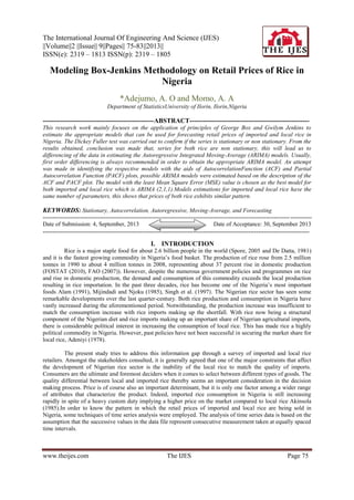
  • 3. Modeling Box-Jenkins Methodology on Retail… www.theijes.com The IJES Page 77 4. The ACF contains small autocorrelations at all lags and the PACF contains small autocorrelations at all lags; use q=0 and p=0. 5. The ACF dies down and the PACF dies down; use p=1 and q=1. Estimating the parameters for the Box–Jenkins models is a quite complicated non-linear estimation problem. For this reason, the parameter estimation should be left to a high quality software program that fits Box–Jenkins models. The main approaches to fitting Box–Jenkins models are non-linear least squares and maximum likelihood estimation (MLE). The MLE is generally the preferred technique, see George et al. (1994). Model diagnostics for Box–Jenkins models is similar to model validation for non-linear least squares fitting. That is, the error term At is assumed to follow the assumptions for a stationary univariate process. The residuals should be white noise drawings from a fixed distribution with a constant mean and variance. If the Box–Jenkins model is a good model for the data, the residuals should satisfy these assumptions. If these assumptions are not satisfied, one needs to fit a more appropriate model. That is, go back to the model identification step and try to develop a better model. One way to assess if the residuals from the Box–Jenkins model follow the assumptions is to generate statistical graphics (autocorrelation plots) of the residuals, see George et al. (1994) andHarris and Robert (2003). Empirical Illustration Using Imported and Local Rice Data To analyze the data for imported rice, the plot that displayed the features (pattern) in which the retail prices of imported rice occurs in Nigeria is shown below, the prices are expressed in naira (#) per one kilogram. Figure 1:Time plot for the retail price of imported rice From the time plot, we could easily observe that, the retail prices of imported rice rises gradually from January, 2001 and then dropped in the month of October of the same year. We also observe a sudden rise in the month of December, 2005 and there was a sudden drop in the month of April, 2006. The plot also notified the presence of upward trend in the series. Therefore, differencing will be necessary so as to obtain stationarity. Test for Autocorrelation In order to check if the errors are autoregressive in nature, the Durbin Watson test for autocorrelation was performed. The hypothesis is stated as: H0: no serial correlation vs H1: there is serial correlation. Table 1: Regression table Source | SS df MS Number of obs = 72 -------------+------------------------------ F( 1, 70) = 865.82 Model | 28771.8523 1 28771.8523 Prob > F = 0.0000 Residual | 2326.14773 70 33.2306818 R-squared = 0.9252 -------------+------------------------------ Adj R-squared = 0.9241 Total | 31098 71 438 Root MSE = 5.7646 ------------------------------------------------------------------------------ month | Coef. Std. Err. t P>|t| [95% Conf. Interval] -------------+---------------------------------------------------------------- imported | .8214094 .0279155 29.42 0.000 .7657337 .8770851 _cons | -40.87836 2.716032 -15.05 0.000 -46.29532 -35.46141 Durbin-Watson d-statistic (2, 72) = 0.9515258 Decision: dcal (0.9515) is less than dtab (1.57), since d is substantially less than 2, we reject HO and conclude that there is an evidence of positive autocorrelation. 6080 100120140 imported 0 20 40 60 80 m onth
  • 4. Modeling Box-Jenkins Methodology on Retail… www.theijes.com The IJES Page 78 Test for stationarity The Dickey Fuller test is used to check for stationarity in series for retail prices of imported rice. The hypothesis statement is stated below; Decision Rule: If the test statistics Z(t) is less than the critical value (usually 10% CV), we reject Ho and conclude that the series is stationary. Table 2 Dickey-Fuller Test Test 1% Critical 5% Critical 10% Critical Statistic Value Value Value Z(t) -1.352 -3.551 -2.913 -2.592 Decision: Since -1.352 > -2.592, we do not reject the hypothesis and we then conclude that there is a unit root in the series. In order to fit the appropriate models, one does not explicitly remove seasonality and trend before fitting the model. Instead, one includes the order of the seasonal terms in the model specification to the ARIMA estimation software. Box and Jenkins recommend the differencing approach to achieve stationarity. The first order differencing (d=1) will be preferred when fitting the ARIMA models. Estimation of ARIMA Models Before we can estimate ARIMA models, we first identify the order of the models with the aids of autocorrelation function (ACF) and partial autocorrelation functions (PACF). The ACF and PACF plots are displayed below; Figure 2 Autocorrelation function plot Figure 3 Partial Autocorrelation function plot -1.00-0.50 0.000.501.00 imported 0 5 10 15 20 25 l ag Bartlett's formula for MA(q ) 95% confidence bands Autocorrelation function (Imported rice) -1.00-0.50 0.000.501.00 imported 0 5 10 15 20 25 l ag 95% Confidence bands [se = 1/sq rt(n)] Partial Autocorrelation function (Imported rice)
  • 5. Modeling Box-Jenkins Methodology on Retail… www.theijes.com The IJES Page 79 From figure 2, we observe that the autocorrelation function plot exhibit exponential decay. This indicates that the order of Autoregressive model can be identified by using the Partial Autocorrelation function plot. From figure 3, the PACF has significant spikes at lag 1 and lag 2, this suggests fitting of AR (2) and alternative model of MA (1). Also, from the time plot (figure 1), we noticed an upward trend in the series, this call for fitting of mixed model with differencing of order one, ARIMA (2,1,1) Table 3 Estimation of AR (2) Model Number of obs = 72 Log likelihood = -128.3527 ------------------------------------------------------------------------------ month | Coef. Std. Err. z P>|z| [95% Conf. Interval] -------------+---------------------------------------------------------------- imported | .1145121 .0278579 4.11 0.000 .0599116 .1691126 _cons | 54.79285 23.61363 0.75 0.451 48.48901 66.07472 -------------+---------------------------------------------------------------- AR: L1| .8620397 .0849272 10.15 0.000 .6955854 1.028494 L2 | .1366306 .0851152 1.61 0.108 -.0301921 .3034534 -------------+---------------------------------------------------------------- The fitted autoregressive model of order 2 is given as: 𝑋𝑡 = 54.7929 + 0.8620𝑋𝑡−1 + 0.1366𝑋𝑡−2 Table 4: Estimation of MA (1) model Number of obs = 72 Log likelihood = -220.8093 ------------------------------------------------------------------------------ month | Coef. Std. Err. z P>|z| [95% Conf. Interval] -------------+---------------------------------------------------------------- imported | .7857546 .0312593 25.14 0.000 .7244874 .8470218 _cons | 47.31309 3.396736 -10.98 0.000 43.97057 63.65561 -------------+---------------------------------------------------------------- MA L1 | .3692167 .1038579 3.56 0.000 .165659 .5727745 -------------+---------------------------------------------------------------- The fitted MA (1) model can be estimated as: 𝑋𝑡 = 47.3131 + 0.3692𝑎𝑡−1 TABLE 5: Estimation of ARMA (2,1) model Number of obs = 72 Log likelihood = -158.2870 ------------------------------------------------------------------------------ month | Coef. Std. Err. z P>|z| [95% Conf. Interval] -------------+---------------------------------------------------------------- imported | .2931712 .0461779 6.35 0.000 .2026641 .3836783 _cons | 59.543362 22.18396 0.43 0.667 33.9364 73.02312 -------------+---------------------------------------------------------------- AR: L1 | .6109667 .2496642 2.45 0.014 .1216338 1.1003 L2 | .3834428 .2452636 1.56 0.118 -.0972649 .8641506 MA: L1 | -.1130025 .2568081 -0.44 0.660 -.616337 .3903321 -------------+---------------------------------------------------------------- The fitted ARMA (2,1) model can be given as: 𝑋𝑡 = 59.5434 + 0 .6110𝑋𝑡−1 + 0.3834𝑋𝑡−2 − 0.1130025𝑎𝑡−1 Table 6: Estimation of ARIMA (2,1,1) model Number of obs = 71 Log likelihood = -225.4229 D.imported | Coef. Std. Err. z P>|z| [95% Conf. Interval] -------------+---------------------------------------------------------------- _cons | .8786367 .4729777 1.86 0.063 -.0483826 1.805656 -------------+---------------------------------------------------------------- AR: L1| -1.474065 .1839555 -8.01 0.000 -1.834611 -1.113518 L2| -.5787382 .0902008 -6.42 0.000 -.7555285 -.401948 MA: L1| 1.032651 .2629669 3.93 0.000 .5172454 1.548057 -------------+---------------------------------------------------------------- The fitted ARIMA (2,1,1) model can be estimated as:
  • 6. Modeling Box-Jenkins Methodology on Retail… www.theijes.com The IJES Page 80 𝑋𝑡 = 0.8786 − 1.4741𝑋𝑡−1 − 0.5787𝑋𝑡−2 + 1.0327𝑎𝑡−1 In order to choose the best model, the Mean Square Error (MSE) Criterion for model selection is adopted. The preferred model is the one with the minimum MSE value. This can be simply expressed as:MSE = SSE/DF Where SSE is the sum of square errors and DF means the degree of freedom. DF can be expressed as: n-p. Where n is the number of observations and p is the number of parameters in the model. The comparison of the results is displayed in the table below: Table 7: Comparison of the Estimated Models Model MSE AR (2) 65.62 MA (1) 264.7 ARMA (2,1) 43.11 ARIMA (2,1,1) 36.01 From the table above, we observe that, ARIMA (2,1,1) has the least MSE value, this model is chosen as the best. Analysis for the Prices of Local Rice Figure 4: Time plot for the retail price of local rice From the time plot, we can easily observe that, the retail prices of local rice rises and drops with a gradual process from the first month. The plot also notified the presence of upward trend in the series. 4.7 TEST FOR AUTOCORRELATION Table 8: Regression table on Local Rice Source | SS df MS Number of obs = 72 -------------+------------------------------ F( 1, 70) = 473.96 Model | 27096.1233 1 27096.1233 Prob > F = 0.0000 Residual | 4001.87668 70 57.1696669 R-squared = 0.8713 -------------+------------------------------ Adj R-squared = 0.8695 Total | 31098 71 438 Root MSE = 7.5611 ------------------------------------------------------------------------------ month | Coef. Std. Err. t P>|t| [95% Conf. Interval] -------------+---------------------------------------------------------------- local | 1.102371 .0506357 21.77 0.000 1.001381 1.203361 _cons| -41.12178 3.675101 -11.19 0.000 -48.45154 -33.79202 ------------------------------------------------------------------------------ Durbin-Watson d-statistic (2, 72) = 0.7265975 Decision: Since d (0.7266) is less than the critical value (dL,α= 1.57), we reject Ho and conclude that the error terms are autoregressive in nature. 406080 100120 local 0 20 40 60 80 month
  • 7. Modeling Box-Jenkins Methodology on Retail… www.theijes.com The IJES Page 81 Test for Stationarity Table 9 Dickey-Fuller Test Test 1% Critical 5% Critical 10% Critical Statistic Value Value Value ------------------------------------------------------------------------------ Z(t) -1.622 -3.551 -2.913 -2.592 Decision: Since -1. 622 > -2.592, we do not reject the hypothesis and we then conclude that there is a unit root in the series. Estimation of ARIMA Models for Local Rice The plots for the calculated ACF and PACF values are displayed below for the purpose of model identification. Figure 5: Autocorrelation function Figure 6: Partial Autocorrelation function The ACF plot in figure 4.8.1, exhibits exponential decay. The order of Autoregressive model can be identified by the plot Partial Autocorrelation function. Both figures suggest fitting of AR (2), MA (1) and ARIMA (2,1). Table 10: Estimation of AR (2) model Number of obs = 72 Log likelihood = -132.2155 ------------------------------------------------------------------------------ month | Coef. Std. Err. z P>|z| [95% Conf. Interval] -------------+---------------------------------------------------------------- local | .1736396 .0414548 4.19 0.000 .0923896 .2548895 _cons | 48.132846 14.42854 0.56 0.573 20.14657 56.41226 -------------+---------------------------------------------------------------- AR L1 | .8220907 .1351067 6.08 0.000 .5572865 1.086895 L2 | .174355 .1406584 1.24 0.215 -.1013303 .4500403 -------------+---------------------------------------------------------------- The fitted AR (2) model is given as: 𝑋𝑡 = 48.1328 + 0 .8221𝑋𝑡−1 + 0.1744𝑋𝑡−2 -1.00-0.50 0.000.501.00 acf 0 5 10 15 20 25 l ag Bartlett's formula for MA(q ) 95% confidence bands Autocorrelation function (local rice) -0.50 0.000.501.00 pacf 0 5 10 15 20 25 l ag 95% Confidence bands [se = 1/sq rt(n)] Partial autocorrelation function (local rice)
  • 8. Modeling Box-Jenkins Methodology on Retail… www.theijes.com The IJES Page 82 TABLE 11: Estimation of MA (1) model Number of obs = 72 Log likelihood = -236.8481 ------------------------------------------------------------------------------ month | Coef. Std. Err. z P>|z| [95% Conf. Interval] -------------+---------------------------------------------------------------- local | 1.023605 .0655703 15.61 0.000 .8950894 1.15212 _cons | 35.33241 4.900818 -7.21 0.000 25.72698 48.75634 -------------+---------------------------------------------------------------- MA L1 | .4193208 .1013462 4.14 0.000 .2206858 .6179558 -------------+-------------------------------------------------------------- The fitted MA (1) model can be estimated as: 𝑋𝑡 = 35.3324 + 0.4193𝑎𝑡−1 TABLE 12: Estimation of ARMA (2,1) model Number of obs = 72 Log likelihood = -172.428 month | Coef. Std. Err. z P>|z| [95% Conf. Interval] -------------+---------------------------------------------------------------- local | .4189884 .0593169 7.06 0.000 .3027294 .5352473 _cons | 38.02211 295.0786 0.23 0.818 21.3214 84.3656 -------------+---------------------------------------------------------------- AR L1 | .4357787 .5478283 0.80 0.426 -.6379451 1.509502 L2 | .5599945 .5496435 1.02 0.308 -.5172868 1.637276 MA L1 | .2019025 .5906723 0.34 0.732 -.9557939 1.359599 -------------+---------------------------------------------------------------- sigma | 2.866552 .3713929 7.72 0.000 2.138635 3.594468 The fitted ARMA (2,1) model can be estimated as: 𝑋𝑡 = 38.0221 + 0.4358 𝑋𝑡−1 + 0.5560𝑋𝑡−2 + 0.2019𝑎𝑡−1 TABLE 13: Estimation of ARIMA (2,1,1) model Number of obs = 71 Log likelihood = -219.3419 ------------------------------------------------------------------------------ D.local | Coef. Std. Err. z P>|z| [95% Conf. Interval] -------------+---------------------------------------------------------------- _cons | .6161748 .5599209 1.10 0.271 -.4812499 1.7136 -------------+---------------------------------------------------------------- AR L1| -1.361776 .3555533 -3.83 0.000 -2.058648 -.6649046 L2| -.3706954 .2269425 -1.63 0.102 -.8154945 .0741037 MA L1| .9471462 .3566943 2.66 0.008 .2480382 1.646254 𝑋𝑡 = 0.6162 − 1.3618𝑋𝑡−1 − 0.3707𝑋𝑡−2 + 0.9471𝑎𝑡−1 From Table (14) below, we observe that, ARIMA (2,1,1) has the least MSE value. Therefore, this model is chosen as the best for forecasting retail prices of imported rice in Nigeria. Table 14:Comparison Of The Estimated Models Model MSE AR (2) 70.0 MA (1) 148.5 ARMA (2,1) 44.18 ARIMA (2,1,1) 35.14 III. CONCLUSION Based on the outcome of the results of the analysis, conclusion can be made, since the aim of this work is to know the pattern of feature that is/are present in the retail prices of rice in Nigeria and also to estimate the
  • 9. Modeling Box-Jenkins Methodology on Retail… www.theijes.com The IJES Page 83 best model for the commodities. From the analysis of local rice, we observed from the time plot, the presence of upward trend before fitting the suggested models, with the use of MSE as the criterion for model selection. We then concluded that ARIMA (2,1,1) 𝑋𝑡 = 0.8786 − 1.4741𝑋𝑡−1 − 0.5787𝑋𝑡−2 + 1.0327𝑎𝑡−1 is the best model that can be used for forecasting retail prices of local rice in Nigeria. Also, from the analysis of imported rice, we also observed from the time plot, the presence of upward trend but not as obvious as that of imported rice. Choosing the minimum value of MSE, conclusion is made that, ARIMA (2,1,1) 𝑋𝑡 = 0.6162 − 1.3618𝑋𝑡−1 − 0.3707𝑋𝑡−2 + 0.9471𝑎𝑡−1 is the best model that can be used for forecasting retail prices of imported rice in Nigeria. In general, our finding shows that more of imported rice is consumed than the local rice in Nigeria, the reason is that, the upward trend in imported rice is higher compared to that of local rice. REFERENCES [1]. Adeniyi, J.P.Rice Industry in Kwara State of Nigeria. An Economic Analysis unpublished Ph. D. Dissertation, University of Ibadan, (1978). [2]. Akinsola, E.A. Problems and Prospects of Rice Varietal resistance Pest Control in West Africa. Insects Sci. Applic. 8, (1985) pp: 467-471. [3]. Alam, M. S. A survey of rice insects pests in Nigeria. Trop. Pest Management 38 (2) (1991), pp. 115-118. [4]. Brockwell, Peter J. and Richard A. Davis. Time Series: Theory and Methods. New York: Springer–Verlag (1987). [5]. Chatfield, Christopher. The Analysis of Time Series: An Introduction. New York, NY: Chapman and Hall (1984). [6]. De Datta, S.K.Principles and practices of rice production. John Wiley and Sons, London (1981). [7]. Delurgio, S.A. Forecasting Principles and Applications. First Edition, Irwin/McGraw Hill Boston, ISBN-10: 0256134332, (1998) pp: 802 [8]. FAO . The state of Food and Agriculture: A Framework document, Rome, available at http://www.fao.org/doc/rep/010. (2007) [9]. FOSTAT. Journal of Agriculture and Social Research, Vol. 10, N02. Also available at http//www.faostatfao.org (2010) [10]. George Box, Gwilym M. Jenkins, and Gregory C. Reinsel.Time Series Analysis: Forecasting and Control, third edition. Prentice- Hall(1994). [11]. Harris, Richard and Robert Sollis. Applied Time Series Modelling and Forecasting. Hoboken, NJ: John Wiley & Sons Inc (2003). [12]. Hurvich, C. M., and Tsai, C.-L. Regression and time series model selection in small samples, Biometrika, 76 (1989): 297–307. [13]. Mijindadi, N. B. and Njoku J. E. Adoption of new technologies by agricultural cooperatives Rice Societies in Kano Nigeria ― International Journal of Development Technology 3 (1985).211-218 [14]. Singh, B.N., S. Fagade, M.N. Ukwungwu, C. Williams, S.S. Jagtap, O. Oladimeji, A. Efisue, & O. Okhidievbie. Rice growing environments and biophysical constraints in different agroecological zones of Nigeria (1997). [15]. Spore (2005). Rice: A success story for some: CTA BI-monthly Magazine. A publication of Technical centre for Agriculture and Rural Cooperation, 115 (2005): pp 4-5.