1. International Journal of Plasticity 26 (2010) 1746–1771
Contents lists available at ScienceDirect
International Journal of Plasticity
journal homepage: www.elsevier.com/locate/ijplas
A plastic constitutive equation incorporating strain, strain-rate,
and temperature
Ji Hyun Sung a, Ji Hoon Kim b, R.H. Wagoner c,*
a
Department of Mechanical Engineering, The Ohio State University, 2041 College Road, Columbus, OH 43210, USA
b
Materials Deformation Group, Korea Institute of Materials Science, 531 Changwondaero, Changwon, Gyeongnam 641-831, South Korea
c
Department of Materials Science and Engineering, The Ohio State University, 2041 College Road, Columbus, OH 43210, USA
a r t i c l e i n f o a b s t r a c t
Article history: An empirical plasticity constitutive form describing the flow stress as a function of strain,
Received 24 November 2009 strain-rate, and temperature has been developed, fit to data for three dual-phase (DP)
Received in final revised form 12 February 2010 steels, and compared with independent experiments outside of the fit domain. Dubbed
Available online 15 March 2010
the ‘‘H/V model” (for ‘‘Hollomon/Voce”), the function consists of three multiplicative func-
tions describing (a) strain hardening, (b) strain-rate sensitivity, and (c) temperature sensi-
Keywords: tivity. Neither the multiplicative structure nor the choice of functions (b) or (c) is novel. The
Constitutive equation
strain hardening function, (a), has two novel features: (1) it incorporates a linear combina-
Work hardening
Dual-phase (DP) steel
tion coefficient, a, that allows representation of Hollomon (power law) behavior (a = 1),
Thermal–mechanical FE simulation Voce (saturation) behavior (a = 0) or any intermediate case (0 < a < 1, and (2) it allows
Deformation-induced heating incorporation of the temperature sensitivity of strain hardening rate in a natural way by
allowing a to vary with temperature (in the simplest case, linearly). This form therefore
allows a natural transition from unbounded strain hardening at low temperatures toward
saturation behavior at higher temperatures, consistent with many observations. Hollomon,
Voce, H/V models and others selected as representative from the literature were fit for
DP590, DP780, and DP980 steels by least-squares using a series of tensile tests up to the
uniform strain conducted over a range of temperatures. Jump-rate tests were used to probe
strain rate sensitivity. The selected laws were then used with coupled thermo-mechanical
finite element (FE) modeling to predict behavior for tests outside the fit range: non-isother-
mal tensile tests beyond the uniform strain at room temperatures, isothermal tensile tests
beyond the uniform strain at several temperatures and hydraulic bulge tests at room tem-
perature. The agreement was best for the H/V model, which captured strain hardening at
high strain accurately as well as the variation of strain hardening with temperature. The
agreement of FE predictions up to the tensile failure strain illustrates the critical role of
deformation-induced heating in high-strength/high ductility alloys, the importance of hav-
ing a constitutive model that is accurate at large strains, and the implication that damage
and void growth are unlikely to be determinant factors in the tensile failure of these alloys.
The new constitutive model may have application for a wide range of alloys beyond DP
steels, and it may be extended to larger strain rate and temperature ranges using alternate
forms of strain rate sensitivity and thermal softening appearing in the literature.
Ó 2010 Elsevier Ltd. All rights reserved.
* Corresponding author. Tel.: +1 614 292 2079; fax: +1 614 292 6530.
E-mail address: wagoner.2@osu.edu (R.H. Wagoner).
0749-6419/$ - see front matter Ó 2010 Elsevier Ltd. All rights reserved.
doi:10.1016/j.ijplas.2010.02.005

2. J.H. Sung et al. / International Journal of Plasticity 26 (2010) 1746–1771 1747
1. Introduction
Advanced high strength steels (AHSS) provide remarkable combinations of strength and ductility by careful control of
microstructure of ferrite, martensite, and retained austenite components. Dual-phase (DP) steel microstructures consist of
large islands (of approximately the grain size) of hard martensite embedded in a softer ferrite matrix, thus mimicking a typ-
ical discontinuous composite structure. DP steels are well-established but their widespread adoption has been limited be-
cause die tryouts show that forming failures can occur much earlier than predicted using standard forming limit
diagrams (FLD) and commercial finite element (FE) programs. Unlike failures observed with traditional steels, unexpected
DP steel failures occur in long channel regions of low R/t (bending radius/sheet thickness) as the sheet is drawn over the
die radius while being stretched, bent and straightened. Such failures are often dubbed ‘‘shear fracture” by industrial prac-
titioners (Huang et al., 2008; Sklad, 2008; Chen et al., 2009). Conventional wisdom has attributed this phenomenon to a spe-
cial damage/void growth mechanism, possibly related to the large, hard martensite islands (Takuda et al., 1999; Horstemeyer
et al., 2000; Lee et al., 2004; Sarwar et al., 2006; Wagoner, 2006; Vernerey et al., 2007; McVeigh and Liu, 2008; Xue, 2008;
Sun et al., 2009).
Recent work was conducted by the authors to determine whether such unpredicted forming failures are a result of typical
plastic localization or a special kind of fracture. Draw-bend tests which reproduce the conditions that promote ‘‘shear fail-
ure” were found to exhibit greatly varying formability depending on the strain rate in the test (Wagoner et al., 2009a,b). Fur-
thermore, temperatures of up to 100 °C in sheet regions away from the necking area were measured, much higher than with
typical traditional steels with lower strength/ductility combinations. It became apparent that the role of temperature in the
flow stress, almost universally ignored in standard sheet forming simulations and mechanical property determinations,
might be a critical factor. In order to consider these effects quantitatively, a reliable constitutive equation was needed in
the range of strain, strain rate, and temperature encountered in such tests and forming operations.
1.1. Role of deformation-induced heating in plastic localization
Unlike the uniformly elevated temperature imposed in a warm forming process (usually applied to increase the inherent
ductility of the alloy), the heat caused by plastic deformation in a local region of high strain has a detrimental effect on
mechanical formability because most alloys soften with increasing temperature, and the softening occurs at the eventual
fracture location (Kleemola and Ranta-Eskola, 1979; Ayres, 1985; Lin and Wagoner, 1986; Gao and Wagoner, 1987; Lin
and Wagoner, 1987; Wagoner et al., 1990; Ohwue et al., 1992). The phenomenon can be seen as a kind of ‘‘reverse
strain-rate sensitivity,” because the higher strain rate in an incipient or developed neck tends to increase the flow stress
via strain-rate sensitivity (and thus delay failure) but also tends to decrease the flow stress via the material’s temperature
sensitivity (thus promoting earlier failure) (Wagoner and Chenot, 1997; Ghosh, 2006).
The deformation-induced thermal effects are important at strain rates high enough that heat transfer out of the neck re-
gion is limited. At sufficiently low rates the deformation becomes quasi-isothermal and temperature sensitivity has a neg-
ligible effect. At sufficiently high rates the deformation is quasi-adiabatic and the heat stays where it is generated. Typical
sheet-forming strain rates in the automotive industry are approximately 10/s (Fekete, 2009), which is close to the adiabatic
limit for typical steels. Therefore, the role of temperature sensitivity of flow stress may be important if it is sufficiently high
and the work of deformation (related to flow stress times ductility) is sufficient to raise the temperature significantly. For DP
steels with high strength and ductility, an accurate description of flow stress incorporating temperature may be essential.
Such a description, if verified, may also be useful for a large range of other materials and applications.
1.2. Plastic constitutive equations
The number, range and complexity of plastic constitutive equations proposed for metals are formidable. They take many
forms, depending on application and intent. The application of interest in the current work is metal forming, sheet metal
forming to be more precise. Typical sheet metal formability is related to the resistance to tensile necking, which is in turn
related to the evolution of plastic flow stress in biaxial tensile stress states encountered during the progressive forming.
Through-thickness stress is typically close to zero (i.e. plane stress) until failure is imminent.
Multi-axial aspects of the plastic constitutive response (yield surface shape, size, and location evolution) are often sepa-
rated for convenience from one-dimensional (1-D) aspects that are obtainable from tensile tests carried out at various strain
rates and temperatures. The current interest is in 1-D aspects. Since many material elements undergo strain paths close to
proportional, strain reversal effects such as the Bauschinger effect can be ignored for many applications.
The preponderance of sheet metal forming is carried out at moderate strain rates (up to approximately 10/s (Fekete,
2009)) and nominally room temperature (although excursions of the order of up to 100 °C are possible because of heat gen-
erated deformation and friction during forming (Wagoner et al., 2009a,b)). For most sheet-formed metals of commercial
interest (e.g. steel, aluminum, copper, titanium) under these conditions, strain hardening is the primary material factor
resisting necking, with strain-rate and temperature sensitivity of flow stress being secondary.
As listed in Appendix A, there are integrated constitutive equations relating plastic flow stress with strain, strain rate, and
temperature (which is the focus of the current work). The strain hardening representations (at constant strain rate and

3. 1748 J.H. Sung et al. / International Journal of Plasticity 26 (2010) 1746–1771
temperature) are of two main types (Table 1): those that approach a saturation stress at large strain (e.g. Brown–Anand
(‘‘BA”) model (Anand, 1982, 1985; Brown et al., 1989), MTS model (Kocks, 1976; Mecking and Kocks, 1981; Follansbee
and Kocks, 1988), Modified Bodner–Partom (‘‘BP”) model (Bodner and Partom, 1975; Chen et al., 2008) and Lin-Wagoner
(‘‘LW”) Model (Lin and Wagoner, 1987)) and those that are unbounded at large strain (e.g. Zirilli–Armstrong (‘‘ZA”) model
(Zerilli and Ronald, 1987), Rusinek–Klepaczko (‘‘RK”) model (Klepaczko, 1987; Rusinek and Klepaczko, 2001; Rusinek
et al., 2007) and Khan–Huang–Liang (‘‘KHL”) model (Khan and Huang, 1992; Khan and Liang, 1999; Khan and Zhang,
2000, 2001; Khan et al., 2004; Khan et al., 2007)). The first group may be called, in short, ‘‘saturation” or ‘‘Voce” models (Voce,
1948; Follansbee and Kocks, 1988) while the second may be called ‘‘Hollomon” or ‘‘power-law” models (Hollomon, 1945);
the proper names refer to the simplest empirical versions of these strain hardening forms appearing in the literature, with
three parameters or two parameters, respectively.
The saturation-type laws are typically found suitable for materials at higher homologous temperatures (and most face-
centered cubic (FCC) metals such as aluminum and copper (Mishra et al., 1989; Choudhary et al., 2001) at room temperature)
while power-law-type models are more suitable for body-centered cubic (BCC) metals and at low homologous temperatures.
For example, iron alloys are known to continue strain hardening at strains up to at least 3 (Johnson and Holmquist, 1988).
Integrated constitutive equations may be subdivided in another way: those that accommodate strain hardening rate
changes with temperature changes (e.g. BA model, MTS model, Modified BP model, LW Model and RK model) and those that
do not (e.g. ZA model and KHL model), Table 1. As shown in Table 1, only the saturation-type integrated laws incorporate
strain hardening rates that are sensitive to temperature (beyond fixed multiplicative or additive functions), with one excep-
tion: the RK model. The RK model (2001) incorporates power-law strain hardening with a power, n, that varies in a pre-
scribed manner with temperature as shown in Appendix A. It is similar in concept to the LW model (1987), where strain
hardening parameters in a saturation-like law are allowed to vary linearly with temperature, thus using six material param-
eters (Appendix A).
In addition to the integrated constitutive equations mentioned above, there are myriad ways to choose and combine
otherwise independent basis functions of strain, strain rate and temperature, which may be generally represented as f(e),
gðeÞ, and h(T), respectively, where e is true tensile strain, e is true strain rate, and T is temperature. (See Appendix B for a
_ _
list of typical functions if this kind. The total number of multiplicative combinations for the choices presented there alone
is 126.) The basis functions may be combined multiplicatively (Hutchison, 1963; Kleemola and Ranta-Eskola, 1979; Johnson
and Cook, 1983; Lin and Wagoner, 1986), additively (Wagoner, 1981b; Ghosh, 2006), or by some combination (Zerilli and
Ronald, 1987) thereof. Each material model of these types prescribes the strain hardening at each temperature as a simple
multiple or addition (or combination), rather than allowing for the character or rate of strain hardening to vary with tem-
perature, hence the definition adopted for Table 1 to decide whether strain hardening is a function of temperature or not.
Common choices for the basis functions f(e), gðeÞ, and h(T), are presented in Appendix B. Several of these combinations have
_
been reviewed and fit to tensile data in the literature (Lin and Wagoner, 1986).
1.3. Purpose of the current work
The purpose of the current work is to develop and verify an empirical plastic constitutive model that meets the following
conditions while introducing the minimum number of undetermined parameters:
(1) it reproduces strain hardening accurately at large strain from fitting in the uniform tensile range,
(2) it captures both extreme kinds of strain hardening forms as well as intermediate cases: bounded (power law) and
unbounded (saturation),
(3) it captures the change of strain hardening character and rate depending on temperature, and
(4) it is capable of predicting strain localization and failure under typical sheet forming conditions of strains, strain rates,
and temperatures.
In order to accomplish these goals, a new multiplicative type phenomenological constitutive equation, the H/V model, is
introduced. The H/V model is a linear combination of the Hollomon and Voce strain hardening equations with a tempera-
Table 1
Classification of integrated 1-D plastic constitutive equations that incorporate the effects of strain, strain-rate, and temperature.a
Unbounded-stress at large strain Strain hardening change with temperature
Brown–Anand N Y
MTS N Y
Modified Bodner–Partom N Y
Lin–Wagoner N Y
Zirilli–Armstrong Y N
Khan–Huang–Liang Y N
Rusinek–Klepaczko Y Y
a
For the classification shown in Table 1, whenever the flow stresses for a given strain at two temperatures differ only by a constant ratio or difference,
then the strain hardening rate is deemed not to depend on temperature.

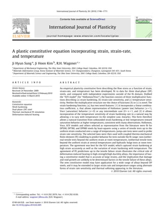
4. J.H. Sung et al. / International Journal of Plasticity 26 (2010) 1746–1771 1749
ture-dependent proportion. The temperature-dependent proportion represents the change of strain hardening character and
rate as temperature changes. Standard multiplicative forms for strain rate sensitivity and thermal softening are incorporated
for fitting and testing. The initial application, the one for which testing is conducted, is for sheet metal forming at rates up to
10/s with deformation-induced heating to temperatures up to 100 deg. C. These are conditions normally encountered in
nominally room-temperature pressforming operations; the application that inspired the current work. Nonetheless, the
H/V model may have application outside of this regime with or without changes in forms to accommodate larger ranges
of strain rate and temperature.
2. H/V constitutive equation
A new empirical work hardening constitutive model, H/V model, is proposed as three multiplicative functions, Eq. (1).
r ¼ rðe; e; TÞ ¼ f ðe; TÞ Á gðeÞ Á hðTÞ
_ _ ð1Þ
Functions f, g, and h together represent the effects of strain, strain rate, and temperature, respectively, on the tensile flow
stress r. g and h are chosen from any of several standard forms (see Appendix B), but the strain hardening function, f, is no-
vel: it incorporates the temperature sensitivity of strain hardening rate via a linear combination of Voce (saturation) (1948)
and Hollomon (power-law) (1945) strain-hardening forms.
2.1. Strain hardening function, f(e,T)
The function f(e, T) represents the major departure and contribution of the new development. The motivation for the
development of f(e, T) is illustrated in Fig. 1(a), which shows strain hardening curves for a dual-phase steel, DP 780, at three
temperatures. To compare the strain hardening curve shapes, the stresses are normalized by dividing by the yield stresses at
each temperature, Fig. 1(b). Clearly the strain hardening rate varies with temperature, being lower at higher temperatures.
This behavior, which is seldom captured by existing constitutive models, is one of the two principal motivations for the cur-
rent development.
In this study, a strain hardening function f(e, T) of the following form is proposed:
f ðe; TÞ ¼ aðTÞfH þ ð1 À aðTÞÞ Á fV ð2Þ
8
> aðTÞ ¼ a1 À a2 ðT À T 0 Þ
<
f ¼ HHV enHV ð3Þ
> H
:
fV ¼ V HV ð1 À AHV eÀBHV e Þ
where T0 is a reference temperature (298 K for simplicity), and a1a2, HHV, nHV, VHV, AHV, and BHV are material constants. The
function a(T) allows a more Voce-like curve at higher temperatures, and a more Hollomon-like curve at lower temperatures
or vice versa, depending on the sign of a1. If a(T) = 1, the H/V model becomes a pure Hollomon model and if a(T) = 0 it be-
comes a pure Voce model. If an intermediate hardening rate is sought that does not depend on temperature, a may be chosen
to be constant: 0 < a0 < 1.
2.2. Strain rate sensitivity function gðeÞ, temperature sensitivity function h(T)
_
The functions gðeÞ and h(T) within the H/V model are not novel; the exact form may be selected from among those
_
appearing in the literature, as listed in Appendix B, or as otherwise devised. It is anticipated that the choice of form of these
functions will not be important over the range of strain rates (up to 10À1/s) and temperatures (25–100 °C) encountered in the
testing carried out in the current work. For extended ranges, the choice of gðeÞ and h(T) may become more clear. The choices
_
of terms gðeÞ and h(T) for the implementation of the H/V model tested in the current work will be explained in more detail in
_
Section 4.1.
3. Experimental procedures
The experiments were chosen to correspond to typical sheet forming practice applied to three DP steels representing a
range of strengths typical of automotive body applications. Constitutive models were fit using standard tensile tests up to
the uniform strain. The quality of the fits was then probed using tensile tests and hydraulic bulge tests to failure.
3.1. Materials
DP steels exhibit good formability and high strength derived from a microstructure that is a combination of a soft ferrite
matrix and a hard martensite phase ‘‘islands.” Three grades of DP steels of nominally 1.4 mm thickness, DP590, DP780, and
DP980, were provided by various suppliers, who requested not to be identified. DP590 was supplied without coating, DP780
with hot-dipped galvanized coating (HDGI), and DP980 with hot-dipped galvanneal coating (HDGA). The chemical

5. 1750 J.H. Sung et al. / International Journal of Plasticity 26 (2010) 1746–1771
1000
25 deg.C
750
50 deg.C
True Stress (MPa)
100 deg.C
500
250
DP780
-3
dε/dt: 10 /s
0
0 0.05 0.1 0.15
True Strain
(a)
2
25 deg.C
Normalized True Stress
50 deg.C
100 deg.C
1.5
DP780
-3
dε/dt: 10 /s
1
0 0.05 0.1 0.15
True Strain
(b)
Fig. 1. Stress–strain response of DP780 at three temperatures: (a) experimental curves and (b) the same data, replotted with the stress divided by the initial
yield stress to reveal strain-hardening differences.
compositions were determined utilizing a Baird OneSpark Optical Emission Spectrometer (HVS-OES) based on ASTM E415-
99a(05) and standard tensile tests were carried out according to ASTM E8-08 at a crosshead speed of 5 mm/min. Both kinds
of tests were conducted at General Motors North America (GMNA, 2007). The chemical compositions and standard ASTM
standard tensile properties appear in Tables 2 and 3, respectively. In order to distinguish normal anisotropies measured from
sheets of the original thickness and those thinned for balanced biaxial testing (as will be discussed in Section 3.5), symbols r1
and r2 in Table 3 refer to sheets of original thickness and thinned thickness, respectively.
Table 2
Chemical composition of dual-phase steels in weight percent (balance Fe).a
C Mn P S Si Cr Al Ni Mo Nb Ti V B
DP590 0.08 0.85 0.009 0.007 0.28 0.01 0.02 0.01 <.01 <.002 <.002 <.002 <.0002
DP780 0.12 2.0 0.020 0.003 0.04 0.25 0.04 <.01 0.17 <.003 <.003 <.003 <.0002
DP980 0.10 2.2 0.008 0.002 0.05 0.24 0.04 0.02 0.35 <.002 <002 <.002 <.0002
a
Chemical analysis was conducted at General Motors North America (GMNA, 2007).

6. J.H. Sung et al. / International Journal of Plasticity 26 (2010) 1746–1771 1751
Table 3
Mechanical properties of dual-phase steels.a
Thickness (mm) 0.2% YS (MPa) UTS (MPa) eu (%) et (%) nb Dr c
r1c r2
d
ad
DP590 1.4 352 605 15.9 23.2 0.21 0.30 0.84 0.98 1.83
DP780 1.4 499 815 12.7 17.9 0.19 À0.11 0.97 0.84 1.86
DP980 1.4 551 1022 9.9 13.3 0.15 À0.23 0.76 0.93 1.90
a
Tests were conducted at General Motors North America (GMNA, 2007) with 5 mm/min crosshead speed at room temp except for test of r2 and a which
were conducted at Alcoa (ATC, 2008; Brem, 2008) with thinned materials.
b
n value was calculated from an engineering strain interval of 4–6%.
c
Dr and r1 were calculated at the uniform strain of original thickness material using Dr = (r0 À 2r45 + r90)/2 and r = (r0 + 2r45 + r90)/4, respectively.
d
r2 value was calculated at the uniform strain of thinned materials using r = (r0 + 2r45 + r90)/4 and a was found by the fit of bulge test result to tensile test
data (using Eq. (9)) considering anisotropy (r2) of thinned materials.
3.2. Material variation
In order to assure uniform, reproducible material properties in this work, a study was undertaken to determine variations
of mechanical properties across the width of a coil. DP steels can exhibit more significant variations in this regard (as com-
pared with traditional mild or HSLA steels) because of the complex thermo-mechanical treatment they undergo during pro-
duction, Fig. 2. The standard deviation of the ultimate tensile stress for DP590 was 25 MPa, a scatter greater than 4% of the
average UTS.
In order to quantify the spatial distribution of material properties and with a goal to minimize such effects on subsequent
testing, numerous rolling direction (RD) tensile tests were conducted with simplified rectangular (non-shouldered) tensile
specimens of DP590 having gage regions between the grips of 125 mm  20 mm. (As will be shown later, see Fig. 4, use
of the rectangular specimens introduces no significant errors up to the uniform elongation.) In order to minimize the effect
of sheared edge quality, the specimen edges were smoothed with 120 grit emery cloth (a practice that was followed for all
tensile tests used in this work). The results from these specimens are summarized in Fig. 3: specimens within 360 mm of the
coil edge (and thus more than 390 mm from the coil center line) exhibit systematic and significant variations in thickness
and UTS, while those in the central region do not. A similar set of tests was performed for a DP980 steel (not the one used
elsewhere in the current work) with the coil width of 1500 mm. The central region more than 300 mm from the edges had
uniform properties. For the three materials used in the current work, DP590 (coil width 1500 mm), DP780 (coil width
1360 mm), DP980 (coil width 1220 mm), only material at least 360 mm from the coil edges was used.
3.3. Tensile testing
ASTM E8-08 sheet tensile specimens with 0% and 1% width taper were initially used for tensile testing, but failures oc-
curred frequently outside of the gage region, thus making the consistent measurement of total elongation problematic.
The failures outside of the gage region were more prevalent at elevated temperatures. In order to obtain consistent test re-
sults, the width taper was increased to 2%, which proved sufficient to insure failure at the center of the specimen for all tests.
As expected (Raghavan and Wagoner, 1987), the increased taper reduced the total elongation, but there was no significant
effect on stress–strain measurement up to the uniform elongation, Fig. 4.
The consistency and reproducibility of tensile results after these two improvements, that is, using material from the cen-
ter of the coil and specimens with 2% width tapers, are illustrated in Fig. 5. The standard variation of UTS is less than 2 MPa
800
Engineering Stress (MPa)
600
σ =567MPa
UTS
400 S.D.=25MPa
200 DP590
Strain rate: 10-2 /s
0
0 5 10 15 20 25 30
Engineering Strain (%)
Fig. 2. Typical range of tensile behavior for DP590 steel specimens selected from various positions across the width of a coil.

7. 1752 J.H. Sung et al. / International Journal of Plasticity 26 (2010) 1746–1771
1.5
DP590 σ =621MPa 640
UTS
1.47 dε/dt: 10 /s
-3 S.D.=2MPa (0.3%)
Thickness (mm)
620
UTS (MPa)
1.44
UTS 600
360mm
1.41
580
1.38
Thickness 560
1.35
0 100 200 300 400 500 600 700
Distance from coil edge (mm)
Fig. 3. Variation of sheet thickness and ultimate tensile strength with position from the edge of a coil (coil width of 1500 mm).
800
Rectangular Specimen
Engineering Stress (MPa)
600
2% Taper
Shouldered
1% Taper
Specimen
400 No Taper
200
DP590
-3
dε /dt: 10 /s
0
0 0.1 0.2 0.3
Engineering Strain
Fig. 4. Effect of tensile specimen geometry on measured stress–strain curves.
1000
DP980
σ = 972MPa, S.D.= 2MPa
Engineering Stress (MPa)
UTS
e =0.139, S.D.= 0.002
f
800 DP780
σ =796MPa, S.D.= 2MPa
UTS
e =0.176, S.D.= 0.002
f
600
DP590
σ = 624MPa, S.D.= 0.7MPa
UTS
e =0.247, S.D.= 0.006
f
400
4 tests per material
2% tapered specimen
-3
dε/dt: 10 /s
200
0 0.1 0.2 0.3
Engineering Strain
Fig. 5. Consistency and scatter of tensile results for three DP steels using 2% tapered tensile specimens and material at least 360 mm away from the edge of
the coil.
(less than 0.3 % of the average value for each material), and the variation of the total elongation is less than 0.006 (less than
2.5% of the average value for each material). In view of these results, specimens with 2% tapers cut from the central region of
the coil were used for all subsequent tensile testing.

8. J.H. Sung et al. / International Journal of Plasticity 26 (2010) 1746–1771 1753
For finding the parameters for the selected constitutive equations, isothermal tensile tests were conducted at 25 °C, 50 °C ,
and 100 °C using a special test fixture designed for tension–compression testing (Boger et al., 2005; Piao et al., 2009). In this
application, the side plates that are pressed against the surface of the specimen (with a force of 2.24 kN) were not required to
stabilize the specimen mechanically against buckling but served instead to heat the specimen for the 50 °C and 100 °C tests
and to maintain near-isothermal conditions throughout the contact length and testing time for all tests. For strain rates up to
10À3/s, the temperature measured in the gage length of the specimen using embedded thermocouples was maintained with-
in 1 °C of the original one up to the uniform strain for all three materials. This method has several advantages compared with
performing tensile tests in air in a furnace, including rapid heat-up (about 3 min to achieve 250 °C), uniform temperature
along the length, and direct strain measurement using a laser extensometer.
The data was corrected for side plate friction (which was minimized using Teflon sheets) and the slight biaxial stress (which
was about 1.5 MPa) using procedures presented elsewhere (Boger et al., 2005). The friction coefficient was determined from the
slope of a least-squares line through the measured maximum force vs. four applied side forces (0, 1.12, 2.24 and 3.36 kN). The
friction coefficients obtained in this way were 0.06, 0.05 and 0.06 for DP590, DP780 and DP980, respectively.
Examples of the tensile testing data at a strain of 10À3/s illustrate the effect of test temperature on the stress–strain
curves (Fig. 6), the yield and ultimate tensile stresses (Fig. 7), and the uniform and total elongations (Fig. 8). The reduced
elongation to failure of higher temperatures is a direct consequence of the lower strain hardening.
For the purpose of comparison with FE simulation, non-isothermal tensile tests were also conducted at a strain rate of
10À3/s in air at room temperature.
3.4. Strain rate jump tests
For materials with limited strain rate sensitivity relative to strength, even small differences of strength from specimen-to-
specimen introduce large relative errors. Jump-rate tensile tests remove specimen-to-specimen variations and thus are pre-
ferred under these conditions. Strain rate jump-down tests, i.e. abruptly changing from a higher strain rate to lower strain
rate, were employed in this study. (Stress–relaxation tests can also remove specimen variations but usually can only be used
for very low strain rates, less than 10À6/s (Wagoner, 1981b).) Fourteen down-jump rate changes, with one jump per tensile
test (Saxena and Chatfield, 1976), were conducted at engineering strains of 0.1, 0.08, 0.06 for DP590, DP780, and DP980
steels, respectively, using the following pairs of rates: 0.5/s ? 0.1/s, 0.5/s ? 0.05/s, 0.1/s ? 0.01/s, 0.1/s ? 0.001/s, 0.05/
s ? 0.01/s, 0.05/s ? 0.005/s, 0.01/s ? 0.001/s, 0.001/s ? 0.0001/s. The jumps 0.1/s ? 0.01/s, 0.01/s ? 0.001/s and 0.001/
s ? 0.0001/s were repeated three times. It has been shown that strain rate sensitivity is nearly independent of strain for
steels (Wagoner, 1981a), which makes jump tests at a single intermediate strain sufficient.
For each down jump, a logarithmic strain rate sensitivity value was determined from the flow stresses r1 and r2 at the
two strain rates e1 and e2 , respectively, for an average strain rate of the two tested strain rates as shown:
_ _
r2 e2 m
_ lnðr2 =r1 Þ
¼ !m¼ ð4Þ
r1 e1
_ lnðe2 =e1 Þ
_ _
pffiffiffiffiffiffiffiffiffi
e
_ av erage ¼ e1 e2
_ _ ð5Þ
The stress after the jump shows a transient response that can be minimized by extrapolating both the higher rate curve
and the lower rate curve to a common true strain 0.005 beyond the jump strain, at which point r1 and r2 are found (Wag-
oner, 1981a). The procedure is illustrated in Fig. 9 for the case of DP590 with a jump from 10À1/s to 10À2/s. The response at
the higher first strain rate over a true strain range of 0.02 is fit to a fourth-order polynomial and extrapolated to the common
800
Engineering Stress (MPa)
Room Temp.
600
o o o
100 C 75 C 50 C
400
200
DP590
-3
dε/dt: 10 /s
0
0 0.1 0.2 0.3
Engineering Strain
Fig. 6. Variation of strain hardening and failure elongation of DP590 with test temperature.

9. 1754 J.H. Sung et al. / International Journal of Plasticity 26 (2010) 1746–1771
50 50
DP780
-3
dε /dt: 10 /s
σ
σ
(MPa)
(MPa)
0 y 0.13 0 y
σ
UTS
0.27 0.34
25 deg.C
25 deg.C
σ
UTS
σ- σ
σ- σ
-50 -50 0.90
DP590
-3
dε /dt: 10 /s
-100 -100
25 50 75 100 25 50 75 100
T (deg. C) T (deg. C)
(a) (b)
50
DP980
dε /dt: 10-3 /s
(MPa)
0
σ
y
25 deg.C
σ 0.48
UTS
σ- σ
-50 0.76
-100
25 50 75 100
T (deg. C)
(c)
Fig. 7. Variation of yield stress and ultimate tensile stress with test temperature: (a) DP590, (b) DP780 and (c) DP980.
strain. The response at the second lower strain rate is similarly fit to a strain range of 0.02 starting at a true strain 0.01 higher
than the jump strain, and is extrapolated to the common strain. The stresses from these extrapolated curves at the common
strain are used to determine the m value from Eq. (4).
3.5. Hydraulic bulge tests
Hydraulic bulge tests were conducted at the Alcoa (ATC, 2008). Because of force limits of the ATC hydraulic bulge test
system, the materials were machined from one side, from an as-received thickness of 1.4 mm–0.5 mm. The stress–strain
response of thinned materials was within standard deviations of 5–10 MPa of the original thickness materials depending
on the material. The die opening diameter was 150 mm and the die profile radius was 25.4 mm. For materials that exhibit
in-plane anisotropy, the stress state near the pole is balanced biaxial tension (Kular and Hillier, 1972) with through-thick-
ness stress negligible for small thickness/bulge diameter ratios (Ranta-Eskola, 1979). In-plane membrane stress, rb, and the
magnitude of thickness strain, et, are given by Eq. (6) and Eq. (7), respectively.
pR
rb ¼ ð6Þ
2t
D
et ¼ 2 ln ð7Þ
D0
where p is pressure, R is a radius of bulge, t is current thickness, D is current length of extensometer, and D0 is the initial
length of the extensometer, 25.4 mm. The radius of curvature R, is measured using a spherometer with each leg located
at a fixed distance of 21.6 mm from the pole. More detailed information for the Alcoa testing machine has appeared else-
where (Young et al., 1981).

10. J.H. Sung et al. / International Journal of Plasticity 26 (2010) 1746–1771 1755
0.2
-3
dε/dt: 10 /s
Temp: 25 deg. C
Uniform Elongation, e u
DP590
0.15
DP780
DP980
0.1
25 50 75 100
T (deg. C)
(a)
0.3
-3
dε/dt: 10 /s
Temp: 25 deg. C
f
Total Elongation, e
DP590
0.2
DP780
DP980
0.1
25 50 75 100
T (deg. C)
(b)
Fig. 8. Ductility change with temperature: (a) uniform elongation (eu) and (b) total elongation (ef).
Fig. 9. Schematic illustrating the procedure for calculating of the strain rate sensitivity, m, for a down jump from 10À1/s to 10À2/s), for DP590 at an
engineering strain of 0.1 (true strain of 0.095).
For an isotropic material, the von Mises effective stress and strain are equal to rb and et, respectively. Because the DP
steels tested here exhibit normal anisotropy, corrections were made for the known normal anisotropy parameters, r2 (the
normal anisotropy was measured using thinned samples at the uniform strain), shown in Table 3 and best-fit values of
the material parameter anisotropy parameter a corresponding to the Hill 1979 non-quadratic yield function (Hill, 1979):

11. 1756 J.H. Sung et al. / International Journal of Plasticity 26 (2010) 1746–1771
2ð1 þ r 2 Þra ¼ ð1 þ 2r 2 Þjr1 À r2 ja þ jr1 þ r2 ja
ð8Þ
The equations for obtaining the appropriate tensile effective stresses and strains for a balanced biaxial stress state have
been presented (Wagoner, 1980):
2r1
r¼
; ¼ e1 ½2ð1 þ r 2 ÞŠ1=a
e ð9Þ
½2ð1 þ r 2 ÞŠ1=a
where e1 is half of the absolute value of the thickness strain. The value of a was found for each material using Eq. (9) and
equating the effective stress and strain from a tensile test and bulge test at an effective strain equal to the true uniform strain
in tension for each material, Table 3.
3.6. Coupled thermo-mechanical finite element procedures
The proposed constitutive equation was tested using a thermo-mechanical FE model of a tensile test with the same spec-
imen geometry as in the experiments. ABAQUS Standard Version 6.7 (ABAQUS, 2007) was utilized for this analysis. One half
of the physical specimen is shown in Fig. 10 with thermal transfer coefficients, but only one-quarter of the specimen was
modeled, as reduced by mirror symmetry in the Y and Z directions. Eight-noded solid elements (C3D8RT) were used for cou-
pled temperature-displacement simulations with two element layers through the thickness. The grip was modeled as a rigid
body.
A von Mises yield function and the isotropic hardening law were adopted for simplicity in view of the nearly proportional
uniaxial tensile stress path throughout most of the test and the normal anisotropy values near unity for the DP steels, Table
Fig. 10. FE model for tensile test: (a) schematic of the model with thermal transfer coefficients, (b) central region of the mesh before deformation and (c)
central region of the mesh after deformation.

12. J.H. Sung et al. / International Journal of Plasticity 26 (2010) 1746–1771 1757
3. The 2% tapered specimen geometry required for experimental reproducibility automatically initiates plastic strain local-
ization at the center of the specimen without introducing numerical defects for that purpose. The total elongation (ef) from
each simulation was defined by the experimental load drop at failure. The simulation accuracy was evaluated based on the
comparison of total elongation with experiments at this same load.
3.7. Determination of thermal constants
For thermal–mechanical FE simulation, various thermal constants are required. The following constants were determined
using JMatPro (Sente-Software, 2007) based on chemical composition: thermal expansion coefficient: linear variation from
1.54 Â 10À6/K at 25 °C to 1.58 Â 10À6/K at 200 °C, heat capacity: linear variation from 0.45 J/gK at 25 °C to 0.52 J/gK at 200 °C,
and thermal conductivity: piecewise linear variation of 36.7 W/m K at 25 °C, 36.9 W/m K at 70 °C, 36.8 W/m K at 100 °C and
36 W/m K at 200 °C. Heat transfer coefficient of metal–air contact was measured as 20W/m2 K and heat transfer coefficient
of metal–metal contact were taken from the literature as 5 KW/m2 K (Burte et al., 1990).
A fraction of the plastic work done during deformation is converted to heat, with the remainder stored elastically as de-
fects (Hosford and Caddell, 1983). The relationship between adiabatic temperature rise and plastic work is as follows:
Z
g
DT ¼ rdep ð10Þ
qC p
where g is a fraction of heat conversion from plastic deformation, q is density of the material and Cp is heat capacity at con-
stant pressure. In order to measure g for DP steels, temperatures were recorded during tensile tests using three thermocou-
ples that were capacitance discharge welded onto specimens on the longitudinal centerline at locations at the center and
±5 mm from the center. The specimen was wrapped with glass fiber sheet to establish quasi-adiabatic conditions at a strain
rate of 5 Â 10À2/s. Fig. 11 shows the results for DP590 and the acceptable correspondence to a value of 0.9 for the parameter
g. g was measured only for DP590, but the value 0.9 was used for each of the three materials.
4. Results and discussion
4.1. Determination of best-fit constitutive constants
As shown by the experimental points shown in Fig. 12, the strain rate sensitivity index, m, is not independent of strain
rate for any of the steels, so the power-law model (Eq. (B.8)) and Johnson–Cook rate law (Eq. (B.9)) were rejected as inad-
equate. The Wagoner rate law (Eq. (B.10)) and a simplified version the Wagoner law with a linear variation of m with log-
arithmic value of strain rate, Eq. (11) below, represent the data equally over this strain rate range as shown in Fig. 12, so the
simpler law was selected:
c2 þðc1 =2Þ logðeÁe0 Þ
_ _
e_
r ¼ re_ 0 _ ð11Þ
e0
where re0 is a stress at e0 and c1 and c2 are material constants.
_ _
The linear variation law, Eq. (11), had slightly better correlation coefficients (R2 = 0.94–0.99) than those for the Wagoner
rate law (R2 = 0.82–0.97). The best-fit values for the parameters for each model are shown in Table 4.
800 30
DP590
True Stress
-2
dε/dt: 5X10 /s
Temp. Increase (deg. C)
True Stress (MPa)
600
20
Temp. increase
400
Eq.10, η=1
Eq.10, η=0.9 10
200 Experiment
0 0
0 0.02 0.04 0.06 0.08 0.1 0.12
True Strain
Fig. 11. Flow stress and temperature increase during a tensile test at a nominal strain rate of 5 Â 10À2/s, DP590.

13. 1758 J.H. Sung et al. / International Journal of Plasticity 26 (2010) 1746–1771
Strain rate sensitivity index, m-value
0.02
DP590(Expt.)
DP780(Expt.)
0.015 DP980(Expt.)
DP590(Fit by Eq. B.10)
DP780(Fit by Eq. B.10)
DP980(Fit by Eq. B.10)
0.01
0.005
0
-5 -4 -3 -2 -1
10 10 10 10 10 1
Strain rate, d ε /dt (1/sec )
(a)
Strain rate sensitivity index, m-value
0.02
DP590(Expt.)
DP780(Expt.)
DP980(Expt.)
0.015 DP590(Fit by Eq. 11)
DP780(Fit by Eq. 11)
DP980(Fit by Eq. 11)
0.01
0.005
0
-5 -4 -3 -2 -1
10 10 10 10 10 1
Strain rate, dε /dt (1/sec )
(b)
Fig. 12. Measured strain rate sensitivities, m, and their representation by strain rate sensitivity laws: (a) Wagoner rate law (Wagoner, 1981a) and (b)
linearized version of Wagoner rate law.
Table 4
Parameters describing the strain rate sensitivity according to three laws.
Power law (mavg) Wagoner rate law Linear law
m1 m0 c1 c2
DP590 0.0062 0.162 0.0125 0.0020 0.0103
DP780 0.0050 0.378 0.0263 0.0030 0.0115
DP980 0.0041 0.289 0.0148 0.0021 0.0086
The remainder of the H/V law was fit using results from continuous, isothermal tensile tests in the uniform strain range
conducted at a strain of 10À3/s and at three temperatures: 25, 50, and 100 °C, Fig. 13 (Note that the H/V model reproduces the
variation of strain hardening rate in the application range 25 °C–100 °C, one of the key objectives of this work.). In order to
choose a suitable form for the thermal softening function h(T), three forms were initially compared as shown in Fig. 14:
Linear (Eq. (B.11)), Power Law 1 (Eq. (B.12)), and Johnson–Cook (Eq. (B.14)). As shown in Fig. 14, and not unexpectedly, there
is no significant difference in the accuracy of the fits of these three laws over the small temperature range tested. The Linear
model (Eq. (B.11)) was chosen for the current work as perhaps the more common and simpler choice, but no advantage is
implied. For application over a larger temperature range or for other materials, presumably one of the forms shown in
Appendix B would provide a measurable advantage over the others and thus could be adopted.
With the form of the thermal function determined, the eight optimal coefficients (a1, a2, HHV, nHV, VHV, AHV, BHV, b) may be
determined for the combined function, again using results from the three tensile tests (at three temperatures) for each
material:

14. J.H. Sung et al. / International Journal of Plasticity 26 (2010) 1746–1771 1759
1200
DP980
True Stress (MPa)
1000 H/V Model
DP780
800
50 deg. C 25 deg. C
100 deg. C
DP590
600
Experiment -3
dε/dt: 10 /s
400
0.02 0.04 0.06 0.08 0.1 0.12 0.14 0.16
True Strain
Fig. 13. Comparison of isothermal tensile test data and best-fit H/V model for DP590, DP780, and DP980.
1080
Line h(T) S.D. (MPa)
Eq. B.11 0.4
Eq. B.12 1.2
1060
True Stress (Mpa)
Eq. B.14 0.4
1040
Experiment
1020
DP980
-3
dε/dt: 10 /s, ε: 0.09
1000
0 20 40 60 80 100 120
Temp (deg. C)
Fig. 14. Comparison of temperature dependent functions h(T) for DP980.
f ðe; TÞ Á hðTÞ ¼ ½aðTÞðHHV enHV Þ þ ð1 À aðTÞÞV HV ð1 À AHV eÀBHV e ÞŠ Á ½1 À bðT À T 0 ÞŠ ð12Þ
8
Using the method of least squares, high and low values of each variable were selected as initial values, producing 2 sets
of starting sets of parameters. The approximate range of parameters were known with Hollomon and Voce fit with the mate-
rial data, therefore the initial values of each parameter were selected based on the range. If fit values are out of the range,
new initial values were selected and fit again. The initial values are shown in the Table 5. Best-fit coefficients were found for
each starting set when the absolute value of the difference between the norm of the residuals (square root of the sum of
squares of the residuals), from one iteration to the next, was less than 0.001. The set exhibiting the minimum R2 value
was chosen as optimal, as reported in Table 5. The accuracy of the fit is shown in Table 5 as a standard deviation between
experiment and fit line and illustrated graphically in Fig. 13.
Using identical procedures, except for the RK model which was fit according to a procedure recommended by provided by
its originators (Rusinek, 2009), several alternative constitutive models were fit to the same tensile test and jump test data, as
follows:
1. H/V model with a = 1 (Hollomon strain hardening at all temperatures).
2. H/V model with a = 0 (Voce strain hardening at all temperatures).
3. H/V model with best-fit constant a = ao (H/V strain hardening, independent of temperature).
4. Lin–Wagoner (LW) model (Eq. (A.7)) (Voce hardening dependent on temperature).
5. Rusinek–Klepaczko (RK) model (Eq. (A.10), (A.11)) (Power-law hardening dependent on temperature).
These choices were made to be representative of the major classes of constitutive models, as reviewed in Section 1.2.
Models 1 and 2 are power-law and saturation hardening models, respectively, that are independent of temperature (except
for a multiplicative function to adjust flow stress with temperature). Models 3 and 4 allow strain hardening rates to vary
with temperature within the frameworks of saturation/Voce or power-law/Hollomon forms, respectively.

15. 1760 J.H. Sung et al. / International Journal of Plasticity 26 (2010) 1746–1771
Table 5
Trial and best-fit coefficients of the H/V model.
Trial values fH fV Temp. const. R2
Parameters Low High S.D.(MPa)
DP590 HHV 500 1500 HHV: 1051 VHV: 643.9 a1: 0.818 0.999
nHV 0.05 0.25 nHV: 0.179 AHV: 0.576 a2: 0.00193 S.D. = 0.5
VHV 500 1500 BHV: 22.44 b: 2.7 Â 10À4
AHV 0.1 0.6
BHV 10 40
a1 0.1 0.9
a2 0 0.005
b 0 0.005
DP780 HHV 500 2000 HHV: 1655 VHV: 752.1 a1: 0.507 0.998
nHV 0.05 0.25 nHV: 0.213 AHV: 0.265 a2: 0.00187 S.D. = 2.5
VHV 500 1500 BHV: 30.31 b: 5.8 Â 10À4
AHV 0.1 0.6
BHV 10 40
a1 0.1 0.9
a2 0 0.005
b 0 0.005
DP980 HHV 500 2000 HHV: 1722 VHV: 908.1 a1: 0.586 0.999
nHV 0.05 0.25 nHV: 0.154 AHV: 0.376 a2: 0.00149 S.D. = 0.6
À4
VHV 500 1500 BHV: 39.64 b: 3.9 Â 10
AHV 0.1 0.6
BHV 10 40
a1 0.1 0.9
a2 0 0.005
b 0 0.005
The material parameters for the RK model, Eq. (A.10), were found using a procedure consisting of six steps recommended
by the first author (Rusinek, 2009). Some fundamental constants in RK model: maximum strain rate, minimum strain rate
and melting temperature were first to be taken from the literature (Larour et al., 2007) and the elastic modulus was taken
to be constant because this study only covered the small homologous temperature range. The remaining six steps followed
for fitting the RK model are as follows:
Step 1: rà ðeP ; TÞ in Eq. (A.11) is zero at low strain rate and at critical temperature. In this study rà ðeP ; TÞ ¼ 0 at the strain
_ _
rate of 10À4/s and the temperature of 300 K since those were the lowest values for strain rate and temperature in this
work. Using this strain rate and temperature combination, C1 was calculated.
Step 2: Eq. (A.10) was fit to material data at the strain rate of 10À4/s and temperature of 300 K, in which rà ðeP ; TÞ ¼ 0, thus
_
allowing determination ofA ð10À4 ; 300 KÞ and n ð10À4 ; 300 KÞ.
Step 3: The strain rate sensitivity term, rà ðeP ; TÞ, was fit to jump test results in order to determine C0 and m.
_
Step 4: Aij ðei ; T j Þ and nij ðei ; T j Þ were found at each strain rate and temperature using Eq. (A.10),.
_ _
Step 5: Aðe; TÞ was fit to Aij values to find A0 and A1.
_
Step 6: nðe; TÞ was fit to nij values to find B0 and B1.
_
The optimal fit coefficients, standard deviations, and R2 values of all models are shown in Tables 6 and 7.
The true stress–strain curves for each of these fits for DP780 are shown in Fig. 15. While the differences are small in the
uniform tensile range (consistent with the small standard errors of fit shown in Tables 5–7), the differences become apparent
when extrapolated to higher strains. Strain hardening at strains beyond the tensile uniform range is particularly important
for sheet forming applications with high curvature bending, where bending strains can be large. The transition of strain hard-
ening type of the H/V law from more Hollomon-like at room temperature to progressively more Voce-like behavior at 50 and
100 ° C can be seen by comparing Figures 13a, 13b and 13c.
Tables 5–7 show that the H/V model provided the lowest standard deviations of fit for each material, followed progres-
sively by the three H/V models with constant a, the LW model, and then the RK model. The difficulty of fitting RK model to
the DP steel data has a fundamental origin: the data showed the strain hardening increases with increasing strain rate but
decreases with increasing temperature, while the RK model requires that the effects of increasing strain rate and tempera-
ture have the same sign of effect on the strain hardening rate.
4.2. Comparison of constitutive model predictions with hydraulic bulge tests
Fig. 16 compares the various constitutive models established above from tensile data with results from room-tempera-
ture (25 °C) hydraulic bulge tests. It is apparent visually and from the standard deviations computed over the strain range

16. J.H. Sung et al. / International Journal of Plasticity 26 (2010) 1746–1771 1761
Table 6
Best-fit coefficients of H/V model for a(T) = 1, a(T) = 0, and a(T) = a0.
a(T) = 1a a(T) = a0 b a(T) = 0 a
f(e)h(T) R2 f(e)h(T) R2 f(e)h(T) R2
S.D.(MPa) S.D.(MPa) S.D.(MPa)
DP590 H1: 1039 0.998 a0: 0.875 0.999 V0: 761.45 0.999
n1: 0.186 S.D. = 2.5 H1: 983 S.D. = 0.9 A0: 0.452 S.D. = 2.0
b: 5.4 Â 10À4 n1: 0.166 B0: 14.6
V0: 806.9 b: 5.6 Â 10À4
A0: 0.825
B0: 22.4
b: 5.5 Â 10À4
DP780 H1: 1234 0.997 a0: 0.850 0.997 V0: 940.9 0.997
n1: 0.148 S.D. = 3.2 H1: 1147 S.D. = 2.8 A0: 0.370 S.D. = 3.2
b: 1.0 Â 10À3 n1: 0.175 B0: 17.19
V0: 1521 b: 1.0 Â 10À3
A0: 0.289
B0: 37.7
b: 1.0 Â 10À3
DP980 H1: 1486 0.996 a0: 0.707 0.999 V0: 1111 0.997
n1: 0.135 S.D. = 3.9 H1: 1332 S.D. = 1.3 A0: 0.353 S.D. = 3.2
b: 7.4 Â 10À4 n1: 0.125 B0: 24.33
V0: 2154 b: 7.4 Â 10À4
A0: 0.9
B0: 52.3
b: 7.4 Â 10À4
a
For a(T) = 1 and a(T) = 0, the same initial values in Table 5 were used.
b
For a(T) = a0, the same initial values in Table 5 were used except V0, A0 and B0 which were found out of the range. For these three parameters, 500 and
2500 MPa, 0.1 and 0.9, and 10 and 60 were used for initial values, respectively.
Table 7
Trial and best-fit coefficients of LW and RK models.
LW RK
Trial Values f(e)h(T) R2 f(e)h(T) S.D.(MPa)
S.D. (MPa)
DP590 A: 500, 1500 A: 764.5 0.999 A0: 1072 Tm: 1750 K S.D. = 4.2
B: 0.1, 0.6 B: 0.452 S.D. = 2.5 A1: 0.076 emax : 107 =s
_
C1: À5, À40 C1: À14.3 e0: 0 emin : 10À5 =s
_
C2: À0.2.0 C2: À0.010 B0: 0.184
b: À0.9, À0.1 b: À0.229 B1: À0.043
C0:180.6
C1:0.53
m: 1.53
A0: 1381
A1: 0.245
DP780 A: 500, 1500 A: 960.4 0.998 e0: 0 Tm: 1750 K S.D. = 9.9
B: 0.1, 0.6 B: 0.375 S.D. = 2.7 B0: 0.146 emax : 107 =s
_
C1: À5, À40 C1: À15.2 B1: À0.033 emin : 10À5 =s
_
C2: À0.2. 0 C2: À0.102 C0: 404.3
b: À0.9, À0.1 b: À0.609 C1: 0.53
m: 2.11
DP980 A: 500, 1500 A: 1118 0.999 A0: 1575 Tm: 1750 K S.D. = 10
B: 0.1, 0.6 B: 0.353 S.D. = 1.8 A1: 0.140 emax : 107 =s
_
C1: À5, À40 C1: À23.3 e0: 0 emin : 10À5 =s
_
C2: À0.2. 0 C2: À0.032 B0: 0.134
b: À0.9, À0.1 b: À0.311 B1: À0.025
C0: 289.6
C1: 0.53
m: 1.92
0.03–0.7, 0.03–0.34, and 0.03–0.23 for DP590, DP780 and DP980, respectively, that the full H/V model and H/V model with
the best-fit constant a0 value (independent of temperature) extrapolated to higher strains reproduce the hydraulic bulge test
results with much greater fidelity than either Hollomon or Voce hardening models. Note that the experimental stress–strain

17. 1762 J.H. Sung et al. / International Journal of Plasticity 26 (2010) 1746–1771
behavior for these materials is intermediate between standard Voce and Hollomon laws, and further that the H/V law fit
from the tensile predicts the high-strain behavior much better than the standard ones. This result illustrates the achievement
of one of the principal objectives of the current development predicting large strain, stress–strain curves accurately. It would
be desirable to have data like that shown in Fig. 16 at other temperatures. Unfortunately, the authors are unaware of any
facility capable of elevated temperature balanced biaxial testing of high strength steels.
1100
DP780
Temp: 25 deg. C
Effective Stress (MPa)
-3
1000 dε/dt: 10 /s
900
α(T)=1
α(T)=αo
α(T)=0
800 Tensile Test LW
RK
H/V
700
0.1 0.2 0.3
Effective Strain
(a)
1100
DP780
Temp: 50 deg. C
True Stress (MPa)
-3
1000 dε/dt: 10 /s
Tensile Test
900
α(T)=1
α(T)=αo
α(T)=0
800 LW
RK
H/V
700
0.1 0.2 0.3
True Strain
(b)
1100
α(T)=1 DP780
α(T)=αo Temp: 100 deg. C
α(T)=0
True Stress (MPa)
-3
1000 dε/dt: 10 /s
LW
RK
H/V
900
800
Tensile Test
700
0.1 0.2 0.3
True Strain
(c)
Fig. 15. Comparison of selected constitutive models at various temperatures, DP780: (a) 25 °C, (b) 50 °C and (c) 100 °C.