2. 560 Ibrahim Kaya / ISA Transactions 42 (2003) 559–575
Fig. 1. The Smith predictor control scheme.
Matausek and Micic ͓5͔ who have shown that by
ˇ ´ cesses. Here, it is shown that the structure can also
adding an additional gain the disturbance response be used to control processes with open loop un-
of the Smith predictor can be controlled indepen- stable poles by using a gain only controller in an
dently of the set point response. The result given inner feedback loop.
in Ref. ͓5͔ was later improved by the same authors For autotuning of the proposed Smith predictor
by adding a PD controller, instead of a propor- structure, plant model transfer functions are first
tional only controller, so that a better disturbance obtained using exact limit cycle analysis from a
rejection can be achieved. More recently, Normey- single relay feedback test. Once the plant model
Rico and Camacho ͓6͔ also proposed a new ap- transfer functions are obtained from the relay au-
proach to design dead-time compensators for totuning, the parameters of the PI-PD controller in
stable and integrating processes. the Smith predictor can be calculated from the for-
It has been shown that a PI-PD controller can mulas provided. Excellent performance of the pro-
give better closed loop responses for processes posed PI-PD Smith predictor over some existing
with large time constants ͓7͔, an integrator ͓8͔, or design methods is illustrated by simulations for
unstable open loop poles ͓9͔. In Kaya and Ather- stable, integrating, and unstable process transfer
ton ͓7͔ controller parameters for a PI-PD control- functions.
ler in a Smith predictor scheme were obtained us-
ing standard forms. The difficulty with the design
is to involve a trade-off between selected values of 2. Model parameter estimation
K p and T i , respectively, the gain and integral time
constant of the PI controller in the forward path. Recently, the relay feedback test based identifi-
The aim of this paper is twofold. First, the control- cation, which is used in this paper, has been very
ler design suggested in Kaya and Atherton ͓7͔ is popular. There are several reasons behind the suc-
extended by providing simple tuning rules. The cess of the relay feedback method. First, the relay
provided simple tuning formulas have physically feedback method, as normally used, gives impor-
meaningful parameters, namely, the damping ratio tant information about the process frequency re-
and the natural frequency o to tune a stable sponse at the critical gain and frequency, which
second-order plus dead time ͑SOPDT͒ and an are the essential data required for controller de-
integrating first-order order plus dead-time sign. Second, the relay feedback method is per-
͑IFOPDT͒ plant transfer functions and closed loop formed under closed loop control. If appropriate
time constant to tune an unstable first-order plus values of the relay parameters are chosen, the pro-
dead time ͑UFOPDT͒ plant transfer function. The cess may be kept in the linear region where the
values of the damping ratio and natural fre- frequency response is of interest. Third, the relay
quency o have been obtained based on desired feedback method eliminates the need for a careful
overshoot and the rise time and the value of time choice of frequency, which is the case for tradi-
constant has been obtained based on the user tional methods of process identification, since an
specified settling time. Second, the Smith predic- appropriate signal can be generated automatically.
tor structure given in Kaya and Atherton ͓7͔ were Finally, the method is so simple that operators un-
suggested only for stable and integrating pro- derstand how it works.
3. Ibrahim Kaya / ISA Transactions 42 (2003) 559–575 561
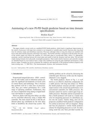
Fig. 2. The proposed Smith predictor control scheme.
Luyben ͓10͔ was one of the first to consider es- K m e ϪL m s
timating the plant transfer function from limit G 1͑ s ͒ ϭ , ͑1͒
͑ T 1m sϩ1 ͒͑ T 2m sϩ1 ͒
cycle measurements and used the approximate de-
scribing function ͑DF͒ method. Several authors K m e ϪL m s
͓11,12͔ have presented further approaches, which G 2͑ s ͒ ϭ , ͑2͒
s ͑ T m sϩ1 ͒
make use of the approximate DF method.
The fact that exact expressions can be found for K m e ϪL m s
a limit cycle in a relay feedback system has been G 3͑ s ͒ ϭ . ͑3͒
T m sϪ1
known for many years ͓13–15͔. Atherton ͓16͔
showed how knowledge of the exact solution for The details of parameter estimation are not given
limit cycles in relay controlled first-order plus here, since interested readers can refer to Kaya
dead time ͑FOPDT͒ plants could be used to give and Atherton ͑Ref. ͓20͔ or Ref. ͓24͔͒ to determine
more accurate results using the DF method. Re- unknown parameters of the related plant transfer
cently, several papers ͓17–19͔ have been written function. However, equations for a stable SOPDT,
on using exact analysis for parameter estimation in IFOPDT, and UFOPDT plant transfer functions to
a relay feedback system, assuming a specific plant identify its unknown parameters are given in the
transfer function and an odd symmetrical limit Appendix for convenience.
cycle. In Kaya and Atherton ͓20͔ asymmetrical
limit cycle data is used, however, the effect of
static load disturbances is not considered. 3. The new PI-PD Smith predictor
Use of expressions based on symmetrical limit configuration
cycles may thus lead to significant errors in the
estimates under static load disturbances, which In the conventional PID control algorithm, the
cause asymmetrical limit cycles. There are only a proportional, integral, and derivative parts are
few works ͓21–23͔ which consider relay autotun- placed in the forward loop, thus acting on the error
ing under static load disturbances. All consider between the set point and closed loop response.
calculation of the ultimate gain and frequency by This PID controller implementation may lead to
first estimating the disturbance and then injecting an undesirable phenomena, namely the derivative
a signal to make the limit cycle odd symmetrical. kick. Also by moving the P͑D͒ part into an inner
Kaya and Atherton ͓24͔ derived exact expressions feedback loop an unstable or integrating process
for the simple features of asymmetrical limit can be stabilized and the pole locations for a stable
cycles in relay controlled loops with both stable process can be modified. Therefore the new PI-PD
and unstable FOPDT and SOPDT plant transfer Smith predictor configuration ͓7͔ is shown in Fig.
functions in the presence of static load distur- 2, where G c1 ( s ) is a PI controller, G c2 ( s ) is a PD
bances. This enables the parameters to be esti- controller, and G d ( s ) is the disturbance rejection
mated directly, which eliminates the need to try to controller. G c2 ( s ) , as mentioned above, is used to
obtain a symmetrical limit cycle. The following stabilize an unstable or integrating process and
transfer functions are used to model a plant trans- modify the pole locations for a stable process. The
fer function by a stable SOPDT, IFOPDT, and other two controllers, G c1 ( s ) and G d ( s ) , are used
UFOPDT, respectively: to take care of servo tracking and regulatory con-
4. 562 Ibrahim Kaya / ISA Transactions 42 (2003) 559–575
trol, respectively. When G c2 ( s ) ϭG d ( s ) ϭ0 then the disturbance response of the Smith predictor
the standard Smith predictor is obtained. can be controlled independently of the controllers
Assuming exact matching between the process G c1 ( s ) and G c2 ( s ) , which are the controllers used
and the model parameters, that is G ( s ) ϭG m ( s ) for servo tracking and designed by using pole zero
and LϭL m , then the set point and disturbance re- cancellations. The controller G d ( s ) , which is used
sponses are given by to control the disturbance rejection, is designed
based on the Nyquist stability criteria. Therefore
C ͑ s ͒ ϭT r ͑ s ͒ R ͑ s ͒ ϩT d ͑ s ͒ D ͑ s ͒ , ͑4͒ both the set point response and disturbance rejec-
tion of the proposed PI-PD Smith predictor result
where
in better performance when compared to existing
G m ͑ s ͒ G c1 ͑ s ͒ e ϪL m s PI͑D͒ Smith predictor controllers.
T r͑ s ͒ ϭ , ͑5͒
1ϩG m ͑ s ͓͒ G c1 ͑ s ͒ ϩG c2 ͑ s ͔͒
G m ͑ s ͒ ͕ 1ϩG m ͑ s ͓͒ G c2 ͑ s ͒ ϩG c1 ͑ s ͒
ϪG c1 ͑ s ͒ e ϪL m s e ϪL m s 4. Development of autotuning formulas
T d͑ s ͒ ϭ .
͕ 1ϩG m ͑ s ͓͒ G c1 ͑ s ͒ ϩG c2 ͑ s ͔͒ ͖
ϫ ͓ 1ϩG d ͑ s ͒ G m ͑ s ͒ e ϪL m s ͔ Case 1: Processes which can be modeled by a
͑6͒ stable SOPDT
For this case, the delay free part of the SOPDT
The transfer function for the set point response, model is
given by Eq. ͑5͒, reveals that the parameters of the
two controllers, G c1 ( s ) and G c2 ( s ) , may be deter-
mined using a model of the delay free part of the Km
G m͑ s ͒ ϭ ͑7͒
plant. In addition, it is seen that only the distur- ͑ T 1m sϩ1 ͒͑ T 2m sϩ1 ͒
bance response T d ( s ) is affected by the controller
G d ( s ) . It has been shown ͓2͔ that the original
Smith predictor gives a steady-state error under and the controllers G c1 ( s ) and G c2 ( s ) have the
disturbances for open loop integrating processes. forms
That is why the controller G d ( s ) has been adopted
in the proposed method, again primarily to im-
prove disturbance rejection for integrating and un-
stable processes transfer functions.
ͩ
G c1 ͑ s ͒ ϭK p 1ϩ
1
T isͪ, ͑8͒
The proposed PI-PD Smith predictor control
structure gives superior performance over classical G c2 ͑ s ͒ ϭK f ͑ 1ϩT f s ͒ . ͑9͒
PI or PID Smith predictor control configuration
for both the set point response and disturbance re- The controller G d ( s ) is not needed in this case as
jection. The superior performance of the proposed the plant is a stable and nonintegrating one. Sub-
Smith predictor is more evident when the process stituting Eqs. ͑7͒–͑9͒ into Eq. ͑5͒, letting T i
has a large time constant, with or without an inte- ϭT 1m and T f ϭT 1m , the delay free part of the
grator or an unstable pole. This is illustrated later closed loop transfer function for the servo tracking
by examples. However, the proposed Smith pre- becomes
dictor configuration still suffers from a mismatch
between the actual process and model dynamics,
which is a case also for classical PI͑D͒ Smith pre- K mK p
dictor scheme. Another point which must be men- T 1m T 2m
tioned about the performance of the proposed T r͑ s ͒ ϭ
1 K mK p
PI-PD Smith predictor design is that one can think s 2ϩ ͑ 1ϩK m K f ͒ sϩ
that due to pole zero cancellation in the controller T 2m T 1m T 2m
design procedure, as will be given in the next sec- 2
o
tion, the load disturbance rejection may be slug- ϭ , ͑10͒
gish. However, as is seen from Eqs. ͑5͒ and ͑6͒, s 2 ϩ2 o sϩ 2
o
5. Ibrahim Kaya / ISA Transactions 42 (2003) 559–575 563
where o and are the natural frequency and h 2 ϭϪ0.6 and ⌬ϭ0 was performed. The static
damping ratio to be specified in the design. Com- load disturbance was assumed to be dϭ0.05. Then
paring the left-and right-hand side of Eq. ͑10͒, measured limit cycle parameters, ϭ0.088, a max
ϭ2.24, a minϭϪ0.64, and ⌬t 1 ϭ35.86, were mea-
T 1m T 2m 2
o sured and used in the identification procedure
K pϭ , ͑11͒
Km given in the Appendix Section 1 to find the
SOPDT model G m1 ( s ) ϭ4e Ϫ14.69s / ( 21.62sϩ1 )
2T 2m o Ϫ1 ϫ( 11.34sϩ1 ) . Fig. 3 illustrates the Nyquist plots
Kfϭ ͑12͒ ¨
Km for the actual plant proposed, Hang’s and Hag-
glund’s obtained models. For this example the
are obtained. The other controller parameters are proposed identification method and the identifica-
T i ϭT 1m ͑13͒ tion method proposed by Hang et al. ͓26͔ gives
quite similar estimation results while the identifi-
and cation method used by Hagglund ͓27͔ gives poor
¨
estimation results. The reason for the identification
T f ϭT 1m . ͑14͒ method proposed by Hang et al. ͓26͔ gives better
When o and in Eqs. ͑11͒ and ͑12͒ are found the estimations is that the time constants used in this
design will be complete. For this, time domain example are larger, which cause the limit cycle
specifications, namely, the maximum overshoot oscillation to be a good sinusoidal and therefore
and the rise time, will be used. The relation be- eliminating the approximation used in the DF
tween the maximum overshoot ͑M͒, the rise time method. The reason for poor estimates obtained by
( T r ) , the damping ratio ͑͒, and the natural fre- ¨
Hagglund is that the open loop step becomes inaf-
quency ( o ) is given ͓25͔ by fective for processes with large time constants.
Specifing a 1% overshoot and 10-s rise time gives
ͱ1Ϫ 2 ϭ0.83 and o ϭ0.2664. The PI-PD controller
M ϭe Ϫ / ͑15͒
parameters K p and K f were calculated as 4.350
and and 1.004, respectively, using Eqs. ͑11͒ and ͑12͒.
The other controller parameters are T i ϭT 1m
1Ϫ0.4167 ϩ2.917 2
T rϭ . ͑16͒ ϭ21.620 and T f ϭT 1m ϭ21.620. The controller
o ¨
parameters for Hang’s and Hagglund’s designs are
Rearranging Eqs. ͑15͒ and ͑16͒, the equations K p ϭ0.0625, T i ϭ15.410 and K p ϭ0.250, T i ϭ31,
respectively. Fig. 4 shows responses for a unity
ϭ ͱ ϩ M M
ln
2
͑
ln ͑
͒2
͒2
͑17͒
step input and disturbance with magnitude of d
ϭϪ0.2 at time tϭ200 s for all three design meth-
ods. The superior performance of the proposed de-
and sign is now clear. Fig. 5 illustrates the good re-
sponse of the proposed structure and design in the
1Ϫ0.4167 ϩ2.917 2 case of Ϯ10% change in the plant time delay.
oϭ ͑18͒
Tr Case 2: Processes which can be modeled by
IFOPDT
can be obtained. Therefore, for the specified maxi- The delay free part of the IFOPDT model is
mum overshoot and rise time, and o can be
found from Eqs. ͑17͒ and ͑18͒, respectively. Once
the value of and o is calculated, K p and K f , Km
respectively, can be found from Eqs. ͑11͒ and ͑12͒. G m͑ s ͒ ϭ . ͑19͒
s ͑ T m sϩ1 ͒
The values of T i and T f are given by Eqs. ͑13͒ and
͑14͒, respectively.
Example 1 The controllers G c1 ( s ) and G c2 ( s ) are again
A fourth-order plant transfer function given given by Eqs. ͑8͒ and ͑9͒. Carrying out the same
by G p1 ( s ) ϭ4e Ϫ10s / ( 20sϩ1 )( 10sϩ1 )( 5sϩ1 )( s procedure as before, the delay free part of the
ϩ1 ) is considered. In order to find the SOPDT closed loop transfer function for servo control, let-
transfer function model the relay test with h 1 ϭ1, ting T i ϭT m and T f ϭT m , is obtained as follows:
6. 564 Ibrahim Kaya / ISA Transactions 42 (2003) 559–575
Fig. 3. Nyquist plots for example 1.
Fig. 4. Step responses for example 1.
7. Ibrahim Kaya / ISA Transactions 42 (2003) 559–575 565
Fig. 5. Step responses for example 1: ͑a͒ for nominal Lϭ10, ͑b͒ for ϩ10% change in the plant time delay, ͑c͒ for Ϫ10%
change in the plant time delay.
K mK p The controller G d ( s ) ,
Tm 2
T r͑ s ͒ ϭ ϭ
o
. G d ͑ s ͒ ϭK d ͑ 1ϩT d s ͒ , ͑25͒
K mK p s 2 ϩ2 o sϩ 2
o
s 2 ϩK f K m sϩ is now necessary for a satisfactory load distur-
Tm
͑20͒ bance rejection. G d ( s ) is designed based on the
stabilization of the second part of the characteris-
Then, one can obtain the controller parameters, by tic equation of Eq. ͑6͒,
comparing the left- and right-hand sides of Eq.
͑20͒, as 1ϩG d ͑ s ͒ G m ͑ s ͒ e ϪL m s ϭ0. ͑26͒
T m 2
o Matausek and Micic ͓28͔ assumed a relation T d
ˇ ´
K pϭ , ͑21͒ ϭ ␣ L m to obtain
Km
2 o /2Ϫ⌽ pm
Kfϭ . ͑22͒ K dϭ
Km K m L m ͱ͑ 1Ϫ ␣ ͒ 2 ϩ ͑ /2Ϫ⌽ pm ͒ 2 ␣ 2
The other controller parameters are ͑27͒
T i ϭT m ͑23͒ for a specified phase margin ⌽ pm . It has to be
noted that ⌽ pm is not the phase margin corre-
and sponding to the system open loop transfer func-
T f ϭT m . ͑24͒ tion. The best results can be obtained ͓28͔ with
␣ ϭ0.4 and ⌽ pm ϭ64°. It should be pointed out
Therefore first and o are, respectively, obtained that Matausek and Micic ͓28͔ use a pure integrator
ˇ ´
from Eqs. ͑17͒ and ͑18͒ and subsequently K p from plus dead-time process model to find K d as given
Eq. ͑21͒ and K f from Eq. ͑22͒. T i and T f are given by Eq. ͑27͒. Therefore, since here the IFOPDT
by Eqs. ͑23͒ and ͑24͒, respectively. model is used, in Eq. ͑27͒ L m ϭT e ϩL m , where T e
8. 566 Ibrahim Kaya / ISA Transactions 42 (2003) 559–575
Fig. 6. Nyquist plots for example 2: ͑a͒ the actual plant, ͑b͒ the proposed model, ͑c͒ the model used by Matausek and Micic.
ˇ ´
is the sum of the equivalent time constants, must ˇ ´
used in Matausek and Micic. The responses to a
be used. unit set point and a disturbance change, which is
Example 2 of magnitude Ϫ0.1 at tϭ50 s, are given in Fig. 7.
An integrating process given by G p2 ( s ) For this example only a small improvement over
ϭe Ϫ5s / s ( s ϩ 1 )( 0.5s ϩ 1 )( 0.2s ϩ1 )( 0.1s ϩ1 ) , ˇ
Matausek’s approach is obtained. Good step re-
which was given in Matausek and Micic ͓28͔, is
ˇ ´ sponses for Ϯ10% mismatch in the plant and
considered. The IFODPT model was obtained as model time delays case, which is the most deterio-
G m2 ( s ) ϭe Ϫ5.72s /s ( 1.18sϩ1 ) using the identifica- rative to system performance, are given in Fig. 8.
tion method given in Appendix Section 3. The re- Example 3
lay parameters were h 1 ϭ1, h 2 ϭϪ0.7 and ⌬ϭ0. Consider G p3 ( s ) ϭe Ϫ6.7s /s ( 10sϩ1 ) , where the
The static load disturbance was assumed to be d plant has both an integrator and a relatively large
ϭ0.2. a maxϭ0.99, a minϭϪ0.69, ϭ0.48, and time constant. The relay parameters used in the
⌬t 1 ϭ6.61 were the measured limit cycle data. relay feedback test were h 1 ϭ1, h 2 ϭϪ0.7, and
Fig. 6 shows the Nyquist plots for the actual plant, ⌬ϭ0. The static load disturbance was assumed to
the model obtained by the proposed method, and be dϭ0.2. With the measured limit cycle data,
ˇ ´
the model used by Matausek and Micic. As is seen a maxϭ0.59, a minϭϪ0.24, ϭ0.29, and ⌬t 1
from the figure both estimation methods result in ϭ11.08, the IFOPDT model was identified ex-
good estimates. Requesting a maximum overshoot actly using the relay estimation method given in
of 1% and a rise time of 5 s gives K p ϭ0.335 and the Appendix Section 3. Fig. 9 shows the Nyquist
K f ϭ0.885, using Eqs. ͑21͒ and ͑22͒. The other plots for the actual plant, the model obtained by
controller parameters are T i ϭT m ϭ1.18 and T f the proposed method, and the model used by Ma-
ϭT m ϭ1.18. K d was calculated from Eq. ͑27͒ as ˇ ´
tausek and Micic. Note that since the model ob-
0.1049, for ␣ ϭ0.4 and ⌽ pm ϭ64°. Also, T d tained by the proposed method matches the actual
ϭ ␣ L m ϭ2.76. Note that here L m ϭT e ϩL m ϭ1.18 plant exactly, its Nyquist plot intersects with the
ϩ5.72ϭ6.9 was used. In Matausek and Micic
ˇ ´ actual plant’s Nyquist plot and hence cannot be
͓28͔ K d ϭ0.1065 and T d ϭ2.72 were used. Also, a ˇ
seen while the model used by Matausek and Micic ´
proportional only controller with gain 0.56 was is quite poor as seen from the figure. The reason
9. Ibrahim Kaya / ISA Transactions 42 (2003) 559–575 567
Fig. 7. Step responses for example 2.
Fig. 8. Step responses for example 2: ͑a͒ for nominal Lϭ5, ͑b͒ for ϩ10% change in the plant time delay, ͑c͒ for Ϫ10%
change in the plant time delay.
10. 568 Ibrahim Kaya / ISA Transactions 42 (2003) 559–575
Fig. 9. Nyquist plots for Example 3: ͑a͒ the actual plant, ͑b͒ the proposed model, ͑c͒ the model used by Matausek and Micic.
ˇ ´
for this is the large time constant. The controller closed loop transfer function for servo control, let-
gains K p and K f were obtained as 2.841 and ting T i ϭT m ϩ2T f and K m K f ϭ2, is obtained as
0.885, respectively, using Eqs. ͑21͒ and ͑22͒, for a follows:
specified value of 1% overshoot and 5-s rise time.
The other controller parameters are T i ϭT m ϭ10 1 1
T r͑ s ͒ ϭ ϭ , ͑29͒
and T f ϭT m ϭ10. Using Eq. ͑27͒, K d ϭ0.0434 was ͑ T i /K m K p ͒ sϩ1 sϩ1
obtained for ␣ ϭ0.4 and ⌽ pm ϭ64°. Also, T d
ϭ ␣ L m ϭ6.68. Matausek’s method ͓28͔ has the
ˇ where is the closed loop design parameter. Let-
same K d and T d values and the main controller ting K m K p ϭ1 results in T i ϭ . Note that it was
gain of 0.1. The responses to a unit set point chosen such that T i ϭT m ϩ2T f . Hence T f ϭ (
change and disturbance of dϭϪ0.1 at tϭ100 s ϪT m ) /2. Therefore the controller parameters are
are given in Fig. 10. The far superior performance given by
of the proposed design method is now evident. 1
Fig. 11 shows the good response of the proposed K pϭ , ͑30͒
structure and design in the case of Ϯ10% change Km
in the plant time delay.
T iϭ , ͑31͒
Case 3: Processes which can be modeled by
UFOPDT 2
The delay free part of the unstable FOPDT is Kfϭ , ͑32͒
given by Km
Km ϪT m
G m͑ s ͒ ϭ . ͑28͒ Tfϭ . ͑33͒
͑ T m sϪ1 ͒ 2
Two main controllers G c1 ( s ) and G c2 ( s ) are The value of , which is the desired closed loop
again given by Eqs. ͑8͒ and ͑9͒. Following a simi- time constant, can be found based on the user
lar procedure as before the delay free part of the specified settling time. The settling time is defined
11. Ibrahim Kaya / ISA Transactions 42 (2003) 559–575 569
Fig. 10. Step responses for example 3.
Fig. 11. Step responses for example 3: ͑a͒ for nominal Lϭ6.7, ͑b͒ for ϩ10% change in the plant time delay, ͑c͒ for Ϫ10%
change in the plant time delay.
12. 570 Ibrahim Kaya / ISA Transactions 42 (2003) 559–575
Fig. 12. Step responses for example 4: ͑a͒ for nominal Lϭ2, ͑b͒ for ϩ10% change in the plant time delay, ͑c͒ for Ϫ10%
change in the plant time delay.
as the time required for the output to settle within of K d is obtained on the basis of stabilization of
a certain percent of its final value. Regardless of second part of characteristic of Eq. ͑6͒,
the percentage used, the settling will be directly
proportional to the time constant for a second- 1ϩK d G m ͑ s ͒ e ϪL m s ϭ0. ͑36͒
order underdamped system ͓29͔. That is,
De Paor and O’Malley ͓31͔ used an optimum
T s ϭk , ͑34͒ phase margin criterion to obtain
where T s is the settling time. In the coefficient
diagram method ͑CDM͒, which is shown to per-
form very well for processes with large time con-
K dϭ
1
Km
ͱT
L
m
m
͑37͒
stants, an integrator or unstable poles k is chosen
with the constraint L m /T m Ͻ1.
between 2.5 and 3.0 ͓30͔. Referring to Eq. ͑34͒
Example 4
and using kϭ2.5,
An unstable process G p4 ( s ) ϭ4e Ϫ2s / ( 4sϪ1 ) is
Ts considered. The plant transfer function was simu-
ϭ ͑35͒ lated in SIMULINK with relay parameters of h 1
2.5
ϭ1, h 2 ϭϪ0.9, and ⌬ϭ0.1. The static load dis-
is obtained. Therefore once the value of is found turbance was assumed to be dϭ0.1. The fre-
from Eq. ͑35͒ with specification on the settling quency of the limit cycle , maximum a max , and
time, the controller parameters can then be found minimum a min of the limit cycle amplitude and the
from Eqs. ͑30͒–͑33͒. pulse duration ⌬t 1 were measured as 0.34, 3.42,
The controller G d ( s ) has to be used again for a Ϫ1.82, and 4.94, respectively. The model was
satisfactory load disturbance rejection. De Paor identified exactly using the identification method
and O’Malley ͓31͔ suggested a proportional only given in the Appendix Section 2, since the as-
controller, G d ( s ) ϭK d , for the stabilization of an sumed model transfer function matches the actual
unstable FOPDT plant transfer function. The value plant transfer function exactly. Letting T s ϭ5s, the
13. Ibrahim Kaya / ISA Transactions 42 (2003) 559–575 571
closed loop time constant is 2.0, from Eq. ͑35͒. 1. Parameter estimation for the SOPDT
Hence the controller parameters are K p ϭ0.25, T i
ϭ2, K f ϭ0.5, and T f ϭϪ1, from Eqs. ͑30͒–͑33͒. Assuming a biased relay and load disturbance at
The parameter of the controller G d ( s ) was found the plant input, two equations for the limit cycle
using Eq. ͑35͒, K d ϭ0.354. With these controller frequency and the pulse duration ⌬t 1 can be
settings, the response of the closed loop system to obtained and are given ͓24͔ by
a unit set point change and a disturbance with
magnitude of Ϫ0.1 at tϭ50 s is given in Fig. 12.
ͩ
The figure also shows the response of the closed
Ϫ ⌬t 1 T 2m e L m /T 2m ͑ 1Ϫe ⌬t 1 /T 2m ͒
loop system in the case of Ϯ10% change in the Km ϩ
plant time delay. As is seen from the figure, the 2 ͑ T 1m ϪT 2m ͒ ͑ e 2 / 2 Ϫ1 ͒
ͪ
proposed Smith predictor structure and design
T 1m e L m /T 1m ͑ 1Ϫe ⌬t 1 /T 1m ͒
method gives very satisfactory results for unstable Ϫ
processes as well. ͑ T 1m ϪT 2m ͒ ͑ e 2 / 1 Ϫ1 ͒
5. Conclusions ϭ
Ϫ
͑ h 1 ϩh 2 ͒ ͩ
dG ͑ 0 ͒ ϩ⌬
ͪ
Simple tuning formulas for a PI-PD Smith pre-
dictor configuration have been given. It is shown G ͑ 0 ͒͑ h 1 ⌬t 1 Ϫh 2 ⌬t 2 ͒
ϩ ͑38͒
by examples that the existing Smith predictor con- P
figurations and design methods for stable and in-
tegrating processes may be ineffective when pro-
cesses include large time constants. Processes with
and
high orders or large time delays have been mod-
eled by lower stable SOPDT, IFOPDT, or
UFOPDT models so that the closed loop system
output will be a second-order response or a first-
order response, where it is proper, assuming a per-
fect matching. The provided simple tuning formu-
Km ͩ ͑ ⌬t 1 Ϫ2 ͒
2
las have physically meaningful parameters, T 2m e L m /T 2m ͑ 1Ϫe ͑ Ϫ ⌬t 1 ϩ2 ͒ / 2 ͒
namely the damping ratio and the natural fre- ϩ
͑ T 1m ϪT 2m ͒ ͑ e 2 / 2 Ϫ1 ͒
quency o for the SOPDT and IFOPDT and time
constant for the UFOPDT. The values of the
damping ratio and natural frequency o have
been obtained based on desired overshoot and the
ϩ
T 1m
͑ T 1m ϪT 2m ͒
e L m /T 1m ͑ 1Ϫe ͑ Ϫ ⌬t 1 ϩ2 ͒ / 1 ͒
͑ e 2 / 2 Ϫ1 ͒
ͪ
rise time and the value of time constant has been
obtained based on the user specified settling time.
The proposed design method has been compared
ϭ
͑ h 1 ϩh 2 ͒ ͩ
dG ͑ 0 ͒ Ϫ⌬
with some existing ones and it is shown by some
examples that the proposed method can be advan-
tageous for processes, either stable or integrating,
ϩ
G ͑ 0 ͒͑ h 1 ⌬t 1 Ϫh 2 ⌬t 2 ͒
P
, ͪ ͑39͒
with large time constants. Also, it is shown that
the proposed Smith predictor configuration and
design method can also be used to control pro- where h 1 and h 2 are the relay heights, ⌬ is the
cesses with unstable plant transfer function. hysteresis. ⌬t 1 and ⌬t 2 are the pulse durations
and Pϭ⌬t 1 ϩ⌬t 2 is the period of the oscillation.
Appendix: Parameter estimation 1 ϭ T 1m , 2 ϭ T 2m and d is the magnitude of
the disturbance.
This section gives equations used to determine Two more equations can be obtained for the
unknown parameters of a stable SOPDT, IFOPDT, maximum and minimum of the plant output wave
or an UFOPDT plant transfer functions based on form which are given by the following equations
relay autotuning. ͓24͔:
14. 572 Ibrahim Kaya / ISA Transactions 42 (2003) 559–575
G ͑ 0 ͒͑ h 1 ⌬t 1 Ϫh 2 ⌬t 2 ͒ before the disturbance enters the system, where
a maxϭdG ͑ 0 ͒ ϩ c ( t ) and y ( t ) are the plant and relay output, re-
P
spectively, and P is the period of the limit cycle.
ϩ
2 ͩ
͑ h 1 ϩh 2 ͒ K m Ϫ ⌬t 1 Once steady-state operation occurs with the dis-
turbance existing, the disturbance magnitude can
be calculated from
T 2m e 1 / 2 ͑ 1Ϫe ⌬t 1 /T 2m ͒
ϩ
͑ T 1m ϪT 2m ͒ ͑ e 2 / 2 Ϫ1 ͒ dϭ
1
G͑ 0 ͒P1
͵ t
tϩ P 1
c ͑ t ͒ dtϪ
h 1 ⌬t 1 Ϫh 2 ⌬t 2
P1
,
Ϫ
T 1m
͑ T 1m ϪT 2m ͒
e 1 / 1 ͑ 1Ϫe ⌬t 1 /T 1m ͒
͑ e 2 / 1 Ϫ1 ͒
, ͪ where P 1 is the period of the limit cycle. The use
͑43͒
of Eq. ͑42͒ to find K m may not be practical. In this
͑40͒ case, the relay test can be performed with its
G ͑ 0 ͒͑ h 1 ⌬t 1 Ϫh 2 ⌬t 2 ͒ heights set to ͉ h 1 ͉ ϭ ͉ h 2 ͉ ϭh so that the disturbance
a minϭdG ͑ 0 ͒ ϩ magnitude can be found using the result given in
P Ref. ͓12͔:
ϩ
ͩ
͑ h 1 ϩh 2 ͒ K m ͑ Ϫ ⌬t 1 ϩ2 ͒
2 dϭ
⌬a
a
h, ͑44͒
T 2m e 2 / 2 ͑ e 2 / 2 Ϫe ⌬t 1 /T 2m ͒ where aϭ ( a maxϩ͉amin͉)/2 and ⌬aϭa maxϪa. Once
ϩ the magnitude of the disturbance is known, Eq.
͑ T 1m ϪT 2m ͒ ͑ e 2 / 2 Ϫ1 ͒
͑43͒ can be rearranged to give
Ϫ
T 1m
͑ T 1m ϪT 2m ͒
e 2 / 1 ͑ e 2 / 1 Ϫe ⌬t 1 /T 1m ͒
͑ e 2 / 1 Ϫ1 ͒
, ͪ K m ϭG ͑ 0 ͒ ϭ ͵ t
tϩ P 1
c ͑ t ͒ dt/ ͑ d P 1 ϩh 1 ⌬t 1
͑41͒
Ϫh 2 ⌬t 2 ͒ . ͑45͒
where For the SOPDT transfer function, Eq. ͑42͒ can be
1ϭ
T 1m T 2m
͑ T 2m ϪT 1m ͒
ln
͑ 1Ϫe
͑ 1Ϫe ͩ
⌬t 1 /T 1m
͒͑ e
͒͑ e
⌬t 1 /T 2m
2 / 2
Ϫ1 ͒
Ϫ1 ͒
2 / 1
ͪ used to find the steady-state gain K m and Eq. ͑43͒
to find the disturbance magnitude d, or Eq. ͑44͒
can be used to find d and then Eq. ͑45͒ to find K m .
Finally, Eqs. ͑40͒ and ͑41͒ may be used to find the
and
time constants T 1m and T 2m . The only remaining
T 1m T 2m unknown, the dead time L m , can then be calcu-
2ϭ lated from either Eqs. ͑38͒ or ͑39͒.
͑ T 2m ϪT 1m ͒
ͩ ͪ
2. Parameter estimation for the UFOPDT
͑ e 2 / 2 Ϫe ⌬t 1 /T 2m ͒͑ e 2 / 1 Ϫ1 ͒
ϫln .
͑ e 2 / 1 Ϫe ⌬t 1 /T 1m ͒͑ e 2 / 2 Ϫ1 ͒ As for the stable SOPDT two equations for the
limit cycle frequency and the pulse duration ⌬t 1
There are five unknowns, namely, K m , T 1m , T 2m ,
͓24͔ are
L m , and d, to be determined. Therefore one more
equation is needed. Fourier analysis can be used to
identify the steady-state gain K and disturbance
magnitude d. It is assumed that the steady-state
Km ͩ ⌬t 1 ͑ e Ϫ⌬t 1 /T m Ϫ1 ͒ e ϪL m /T m
2
Ϫ
͑ e Ϫ2 / Ϫ1 ͒ ͪ
gain can be calculated from
ϭ
Ϫ
͑ h 1 ϩh 2 ͒ ͩ
dG ͑ 0 ͒ ϩ⌬
͵ tϩ P
K ϭG ͑ 0 ͒ ϭ
t
c ͑ t ͒ dt
͑42͒ ϩ
G ͑ 0 ͒͑ h 1 ⌬t 1 Ϫh 2 ⌬t 2 ͒
ͪ ͑46͒
͵ P
m tϩ P
y ͑ t ͒ dt
t and
15. Ibrahim Kaya / ISA Transactions 42 (2003) 559–575 573
Km ͩ ͑ Ϫ ⌬t 1 ϩ2 ͒
2
sumed that there is no disturbance to the system
͓32,33͔. If an unbiased relay test with no load dis-
turbances is performed, either the gain has to be
Ϫ
͑ e ͑ ⌬t 1 Ϫ2 ͒ / Ϫ1 ͒ e ϪL m /T m
͑ e Ϫ2 / Ϫ1 ͒
ͪ assumed known or two relay tests, one with hys-
teresis and another without hysteresis, have to be
performed. However, the standard relay autotun-
ϭ
͑ h 1 ϩh 2 ͒ ͩ
dG ͑ 0 ͒ Ϫ⌬
ing can slightly be improved to determine the un-
known parameters of the IFOPDT using a biased
relay and/or assuming static load disturbances. For
ϩ
G ͑ 0 ͒͑ h 1 ⌬t 1 Ϫh 2 ⌬t 2 ͒
P
, ͪ ͑47͒
this, a differentiator is put in front of the IFOPDT
plant transfer function to cancel the integrator pole
by the zero of the differentiator. In this case, the
where ϭ T m . overall plant transfer function is a stable FOPDT
The other two equations, for the minimum and which has unknown parameters of K m , T m , and
maximum of the plant output, are L m . In theory, differentiating the relay output
gives impulses at zero crossings while in practice
G ͑ 0 ͒͑ h 1 ⌬t 1 Ϫh 2 ⌬t 2 ͒ these impulses can be approximated by pulses
a minϭdG ͑ 0 ͒ ϩ
P with short pulse width. Therefore to identify the
ͩ ͪ
unknown parameters of the IFOPDT, all one needs
͑ h 1 ϩh 2 ͒ K m ⌬t 1 ͑ 1Ϫe Ϫ⌬t 1 /T m ͒ is to derive equations for a stable FOPDT. This is
ϩ ϩ
2 ͑ e Ϫ2 / Ϫ1 ͒ the approach used in this paper and the equations
required can be found in Refs. ͓32,20͔ and are
͑48͒ given here for convenience.
and Equations for the limit cycle frequency and
the pulse duration ⌬t 1 ͓32,20͔ are
G ͑ 0 ͒͑ h 1 ⌬t 1 Ϫh 2 ⌬t 2 ͒
a maxϭdG ͑ 0 ͒ ϩ
P Km ͩ Ϫ ⌬t 1 ͑ e ⌬t 1 /T m Ϫ1 ͒ e L m /T m
2
ϩ
͑ e 2 / Ϫ1 ͒ ͪ
ϩ
ͩ
͑ h 1 ϩh 2 ͒ K m ͑ ⌬t 1 Ϫ2 ͒
2 ϭ
Ϫ
͑ h 1 ϩh 2 ͒ ͩ
dG ͑ 0 ͒ ϩ⌬
ϩ
e ⌬t 1 /T m
͑e
͑e
Ϫ2 /
Ϫ2 /
Ϫe
Ϫ1 ͒
Ϫ⌬t 1 /T m
͒
ͪ .
ϩ
G ͑ 0 ͒͑ h 1 ⌬t 1 Ϫh 2 ⌬t 2 ͒
P ͪ ͑50͒
͑49͒
and
The steady-state gain K m and the disturbance mag-
nitude d are found either using Eqs. ͑42͒ and ͑43͒
or Eqs. ͑44͒ and ͑45͒. The time constant T m can be
obtained from either Eq. ͑48͒ or Eq. ͑49͒. Finally,
Km ͩ ͑ ⌬t 1 Ϫ2 ͒
2
with K m , d, and T m known, the dead time can be
calculated from either Eq. ͑46͒ or Eq. ͑47͒. ϩ
͑ e ͑ Ϫ ⌬t 1 ϩ2 ͒ / Ϫ1 ͒ e L m /T m
͑ e 2 / Ϫ1 ͒
ͪ
3. Parameter estimation for the IFOPDT
Unlike the SOPDT and UFOPDT, the standard
ϭ
͑ h 1 ϩh 2 ͒ ͩ
dG ͑ 0 ͒ Ϫ⌬
relay autotuning under static load disturbances or
with a biased relay cannot be used for parameter ϩ
G ͑ 0 ͒͑ h 1 ⌬t 1 Ϫh 2 ⌬t 2 ͒
P
, ͪ ͑51͒
estimation of the IFOPDT, since in the equations
obtained G ( 0 ) will appear which is infinity for the where ϭ T m .
IFOPDT. Therefore for the IFOPDT an unbiased Two more equations can be calculated from the
relay has to be used. In addition, it has to be as- plant output, one for the maximum of the plant
16. 574 Ibrahim Kaya / ISA Transactions 42 (2003) 559–575
output and the other for the minimum of the plant for integrating processes. Proc. of American Control
output. They are given by Conference, ACC’99, 1999, pp. 258 –262.
͓9͔ Atherton, D. P. and Boz, A. F. Using standard forms
G ͑ 0 ͒͑ h 1 ⌬t 1 Ϫh 2 ⌬t 2 ͒ for controller design. UKACC Int. Conference on
a minϭdG ͑ 0 ͒ ϩ Control’98, Swansea, UK, 1998, pp. 1066 –1071.
P ͓10͔ Luyben, W. L., Derivation of transfer functions for
ͩ
highly nonlinear distillation columns. Ind. Eng. Chem.
͑ h 1 ϩh 2 ͒ K m Ϫ ⌬t 1 Res. 26, 2490–2495 ͑1987͒.
ϩ ͓11͔
2 Li, W., Eskinat, E., and Luyben, W. L., An improved
autotune identification method. Ind. Eng. Chem. Res.
ϩ
͑ e ⌬t 1 /T m Ϫ1 ͒
͑ e 2 / Ϫ1 ͒ ͪ ͑52͒ ͓12͔
30, 1530–1541 ͑1991͒.
Shen, S. H., Wu, J. S., and Yu, C. C., Use of biased-
relay feedback for autotune identification. AIChE J.
42, 1174 –1180 ͑1996͒.
and ͓13͔ Bohn, E. V., Stability margins and steady-state oscil-
lations in on-off feedback systems. IRE Trans. Circuit
G ͑ 0 ͒͑ h 1 ⌬t 1 Ϫh 2 ⌬t 2 ͒ Theory 8, 127–130 ͑1961͒.
a maxϭdG ͑ 0 ͒ ϩ ͓14͔ Chung, J. K.-C. and Atherton, D. P., The determination
P
of periodic modes in relay systems using the state
ϩ
ͩ
͑ h 1 ϩh 2 ͒ K m ͑ Ϫ ⌬t 1 ϩ2 ͒
2
͓15͔
space approach. Int. J. Control 4, 105–126 ͑1966͒.
Atherton, D. P., Conditions for periodicity in control
systems containing several relays. 3rd IFAC Congress,
ͪ
Paper 28E, 1966.
e Ϫ⌬t 1 /T m ͑ e ⌬t 1 /T m Ϫe 2 / ͒ ͓16͔ Atherton, D. P. Improving accuracy of autotuning pa-
ϩ . ͑53͒
͑ e 2 / Ϫ1 ͒ rameters estimation. Proc. IEEE, Int. Conference of
Control App., Hartford, CT, 1997, pp. 51–56.
The steady-state gain K m is again obtained from ͓17͔ Chang, R. C., Shen, S. H., and Yu, C. C., Derivation of
Eq. ͑42͒, and d from Eq. ͑43͒, the time constant transfer functions from relay feedback systems. Ind.
Eng. Chem. Res. 31, 855– 860 ͑1992͒.
T m , can be obtained from either Eq. ͑52͒ or Eq. ͓18͔ Wang, Q. G., Hang, C. C., and Zou, B., Low order
͑53͒. Finally, with K m , T m , and d known, the modeling from relay feedback systems. Ind. Eng.
dead time L m can be calculated from either Eq. Chem. Res. 3, 375–381 ͑1997͒.
͑50͒ or Eq. ͑51͒. ͓19͔ Kaya, I. and Atherton, D. P., Parameter estimation us-
ing limit cycle data. Trans. Inst. Meas. Control ͑Lon-
don͒ 21, 21–29 ͑1999͒.
͓20͔ Kaya, I. and Atherton, D. P., Parameter estimation
References from relay autotuning with asymmetric limit cycle
͓1͔ Smith, O. J., A controller to overcome dead time. ISA data. J. Process Control 11, 429– 439 ͑2001͒.
͓21͔ ˚ ¨
J. 6, 28 –33 ͑1959͒. Hang, C. C., Astrom, K. J., and Ho, W. K., Relay
͓2͔ Watanabe, K. and Ito, M., A process-model control for autotuning in the presence of static load disturbance.
linear systems with delay. IEEE Trans. Autom. Control Automatica 29, 563–564 ͑1993͒.
AC-26, 1261–1266 ͑1981͒. ͓22͔ Shen, S. H., Wu, J. S., and Yu, C. C., Autotune iden-
˚ ¨
͓3͔ Astrom, K. J., Hang, C. C., and Lim, B. C., A new tification under load disturbance. Ind. Eng. Chem. Res.
Smith predictor for controlling a process with an inte- 35, 1642–1651 ͑1996͒.
grator and Long dead-time. IEEE Trans. Autom. Con- ͓23͔ Park, J. H., Sung, S. W., and Lee, I. B., Improved relay
trol 39, 343–345 ͑1994͒. autotuning with static load disturbance. Automatica
͓4͔ Zhang, W. D. and Sun, Y. X., Modified Smith predic- 33, 711–715 ͑1997͒.
tor for integrator/time delay processes. Ind. Eng. ͓24͔ Kaya, I. and Atherton, D. P. Exact parameter estima-
Chem. Res. 35, 2769–2772 ͑1996͒. tion from relay autotuning under static load distur-
͓5͔ Matausek, M. R. and Micic, A. D., A modified Smith
ˇ ´ bances. Proc. of American Control Conference,
predictor for controlling a process with an integrator ACC’01, 2001, pp. 3274 –3279.
and long dead-time. IEEE Trans. Autom. Control 44, ͓25͔ Kuo, B. C. Automatic Control Systems. Prentice-Hall,
1199–1203 ͑1996͒. Englewood Cliffs, NJ, 1995.
͓6͔ Normey-Rico, J. E. and Camacho, E. F., A unified ap- ͓26͔ Hang, C. C., Wang, Q. G., and Cao, L. S., Self-tuning
proach to design dead-time compansators for stable Smith predictors for processes with long dead time.
and integrative processes with dead time. IEEE Trans. Int. J. Adapt. Control Signal Process. 9, 255–270
Autom. Control 47, 299–305 ͑2002͒. ͑1995͒.
͓7͔ Kaya, I. and Atherton, D. P., A new PI-PD Smith pre- ͓27͔ ¨
Hagglund, T., A predictive PI controller for processes
dictor for control of processes with long dead time. with long dead-time delay. IEEE Control Syst. Mag.
14th IFAC World Congress, Vol. C, 1999, pp. 283– 12, 57– 60 ͑1992͒.
288. ͓28͔ ˇ ´
Matausek, M. R. and Micic, A. D., On the modified
͓8͔ Kaya, I. and Atherton, D. P., A PI-PD controller design Smith predictor for controlling a process with an inte-
17. Ibrahim Kaya / ISA Transactions 42 (2003) 559–575 575
grator and long dead-time. IEEE Trans. Autom. Con- ͓31͔ De Paor, A. M. and O’Malley, M., Controllers of Zie-
trol 41, 1603–1606 ͑1999͒. gler Nichols type for unstable processes. Int. J. Con-
͓29͔ Phillips, C. L. and Harbor, R. D., Feedback Control trol 49, 1273–1284 ͑1989͒.
Systems. Prentice-Hall, Englewood Cliffs, NJ, 1996. ͓32͔ Kaya, I. Relay Feedback Identification and Model
͓30͔ Hamamci, S. E., Kaya, I., and Koksal, M. Improving Based Controller Design. Ph.D. thesis, University of
performance for a class of processes using Coefficient Sussex, Brighton, U.K., 1999.
Diagram Method. 9th IEEE Mediterranean Conference ͓33͔ Atherton, D. P. Nonlinear Control Engineering.
on Control and Automation, June 27–29, Dubrovnik, Van Nonstrand-Reinhold, London, Student Edition,
Croatia, 2001. 1981.