SlideShare ist ein Scribd-Unternehmen logo
1 von 72
Downloaden Sie, um offline zu lesen
Chapter 10.                VOF Free Surface Model


                       Information about the VOF model is divided into the following
                       sections:

                            Section 10.1: Introduction
                            Section 10.2: Theory
                            Section 10.3: Using the VOF Model

10.1   Introduction

                  Two models are available in FLUENT for simulations where two or
                  more uids are present. The Volume of Fluid VOF model Hirt
                  and Nichols, 1981 49  is designed for two or more immiscible uids,
                  where the position of the interface between the uids is of interest.
                  The Eulerian model, described in Chapter 9, is designed for two or
                  more interpenetrating uids. Whereas the Eulerian model makes
                  use of multiple momentum equations to describe the individual u-
                  ids, the VOF model does not. In the VOF model, a single set
                  of momentum equations is shared by the uids, and the volume
                  fraction of each of the uids is tracked throughout the domain. Ap-
                  plications of the VOF model include the prediction of jet break-up,
                  the motion of large bubbles in a liquid, the motion of liquid after a
                  dam break, or the steady or transient tracking of any liquid-gas in-
                  terface. The Eulerian multiphase model, on the other hand, is best
                  suited for applications involving slurries or liquid-liquid and liquid-
                  gas mixtures involving small bubbles. The distinction between large
                  and small bubbles in these examples is based on the size of a typical
                  control volume. If a bubble is much smaller than a control volume,
                  many such bubbles can be treated as a separate uid in the Eu-
                  lerian multiphase model. If the bubble is so large that it extends
                  across several control volumes, the VOF formulation is appropriate
                  to track its boundary.
Example of a Dam To illustrate the capabilities of the VOF model, consider a rectan-
            Break gular domain, 4 m long and 2.2 m high, in which water is initially
                  con ned to a region on the left side by the presence of a dam. At
                  time t=0, the dam breaks, and the water starts to ow to the right.
10-2                                       Chapter 10 | VOF Free Surface Model

                   Figures 10.1.1 and 10.1.2 illustrate the spread of the water during
                   the rst 0.7 seconds.
                   By 0.9 and 1.1 seconds, the water has reached the opposite side of
                   the container and is moving up the wall Figure 10.1.3.
                   If the grid is su ciently ne, FLUENT can predict the formation of
                   large water drops that separate from the water stream as it hits
                   the upper boundary of the domain. These drops will then fall to
                   the bottom of the container, where they will reattach to the water
                   there.
  Auxiliary Models Most FLUENT models are available in combination with the VOF
   and Limitations model. For example, the sliding-mesh model can be used to pre-
                   dict the shape of the surface of a liquid in a mixing tank. The
                   deforming mesh capability is also compatible with the VOF model.
                   The porous media model can be used to track the motion of the
                   interface between two uids through a packed bed or other porous
                   region. The e ects of surface tension may be included for one
                   speci ed phase only, and in combination with this model, you can
                   specify the wall adhesion angle. Heat transfer from walls to each
                   of the phases can be modeled, as can heat transfer between phases.
                   Turbulence modeling is available through the standard or the RNG
                   k - -model. Turbulence modeling with the Reynolds Stress model
                   is not available, however. For any of these applications, note that
                   all control volumes must be lled with either a single uid phase
                   or a combination of phases, since the model does not allow for void
                   regions where no uid of any type is present.
                   Some models are available for only one of the phases. Only one
                   phase's density can be calculated using the gas law. Species mix-
                   ing and reacting ow can be modeled in one of the phases, but
                   mass transfer between phases cannot be modeled without User-
                   De ned Subroutines. While temperature-dependent properties are
                   available for both phases, the kinetic theory option is only avail-
                   able for one of the phases, as is property de nition through User-
                   De ned-Subroutines. Only one of the phases can be modeled with
                   a non-Newtonian viscosity law.
                   If you model solidi cation using the phase change model described
                   in Chapter 8, the solidi cation can occur in only one phase. By
                   default, this solidifying phase is the rst secondary phase. You will
                   have the opportunity to specify a di erent phase for solidi cation
                   when you specify the phase change properties see Section 8.3.
                   Note also that solidi cation cannot take place in the vicinity of the
                   interface between two phases.

                                                                       c   Fluent Inc. May 10, 1997
10.1 Introduction                                                                                        10-3


                                   1.00E+00


                                   5.00E-01


                                   0.00E+00

                                    Y         Transient Simulation of a Dam Break                  Oct 20 1994
                                    Z   X     Water Volume Fraction (Dim)                          Fluent 4.30
                                              Lmax = 1.000E+00 Lmin = 0.000E+00 Time = 2.000E-01    Fluent Inc.


                               Figure 10.1.1: Transient Simulation of a Dam Break During the
                               First 0.2 Seconds
                                   1.00E+00


                                   5.00E-01


                                   0.00E+00

                                    Y         Transient Simulation of a Dam Break                  Oct 20 1994
                                    Z   X     Water Volume Fraction (Dim)                          Fluent 4.30
                                              Lmax = 1.000E+00 Lmin = 0.000E+00 Time = 7.000E-01    Fluent Inc.


                               Figure 10.1.2: Transient Simulation of a Dam Break at 0.5 and 0.7
                               Seconds


c   Fluent Inc. May 10, 1997
10-4                                            Chapter 10 | VOF Free Surface Model


                         1.00E+00


                         5.00E-01


                         0.00E+00

                         Y          Transient Simulation of a Dam Break                                Oct 24 1994
                         Z    X     Water Volume Fraction (Dim)                                        Fluent 4.30
                                    Lmax = 1.000E+00 Lmin = 0.000E+00 Time = 1.100E+00                  Fluent Inc.


                    Figure 10.1.3: Transient Simulation of a Dam Break at 0.9 and 1.1
                    Seconds

  Steady State vs. The VOF formulation in FLUENT is, by default, time-dependent,
 Time Dependence but for problems in which you are concerned only with a steady-
                    state solution, it is possible to perform a steady-state calculation.
                    A steady-state VOF calculation is sensible only when your solution
                    is independent of the initial conditions and there are distinct in ow
                    boundaries for the individual phases. For example, since the shape
                    of the free surface inside a rotating cup depends on the initial level of
                    the uid, such a problem must be solved using the time-dependent
                    formulation. On the other hand, the ow of water in a channel with
                    a region of air on top and a separate air inlet can be solved with
                    the steady-state formulation.


                                                                                         c   Fluent Inc. May 10, 1997
10.2 Theory                                                                               10-5

10.2          Theory

                      The VOF formulation relies on the fact that two or more uids
                      or phases are not interpenetrating. For each additional phase
                      that you add to your model, a variable is introduced, which is the
                      volume fraction of that phase. In each control volume, the volume
                      fractions of all phases add to unity. The elds for all variables and
                      properties are shared by the phases, as long as the volume fraction
                      of each of the phases is known at each location. Thus the variables
                      and properties in any given cell are either purely representative of
                      one of the phases, or are representative of a mixture of the phases,
                      depending upon the volume fraction values. In other words, if the
                      volume fraction of the kth uid in a multi- uid system is denoted
                       k , then the following three conditions are possible:

                         k = 0        the cell is empty of the kth uid
                         k = 1        the cell is full of the kth uid
                        0 k 1 the cell contains the interface between the uids
                      Based on the local value of k , the appropriate properties and vari-
                      ables will be assigned to each control volume within the domain.
          The Volume The tracking of the interfaces between the phases is accomplished
    Fraction Equation by the solution of a continuity equation for the volume fraction of
                      one or more of the phases. For the kth phase, this equation has
                      the form:
                                                     @            @
                                                      @t
                                                         k
                                                             + uj @xk = S k            10.2-1
                                                                      i


                            The source term on the right hand side of Equation 10.2-1 is nor-
                            mally zero, but can be constructed with a User-De ned Subroutine
                            to generate a source of the kth phase in one or more regions of the
                            solution domain to simulate mass transfer between phases. This
                            task requires the additional speci cation of a mass source.
                 Properties The properties appearing in the transport equations are determined
                            by the presence of the component phases in each control volume.
                            In a two-phase system, for example, if the phases are represented
                            by the subscripts 1 and 2, and if the volume fraction of the second
                            of these is being tracked, the density in each cell is given by:

                                                      =      2 2   + 1 , 2    1      10.2-2
                               In general, for an N-phase system, the volume-fraction averaged
                               density takes on the form:

c   Fluent Inc. May 10, 1997
10-6                                           Chapter 10 | VOF Free Surface Model

                                                                       X
                                                                  =                k k                                    10.2-3
                       All other properties are computed in this manner viscosity and
                       thermal conductivity, for example with the exception of the speci c
                       heat, which is mass fraction averaged:
                                                                P
                                                                                   k cp k
                                                            cp = P                                                        10.2-4
                                                                  k

                                                                                   k k


                       The basis for the mass-weighted averaging done for the speci c heat
                       lies in the manner in which the enthalpy is calculated at cells near
                       the interface. The enthalpy in general is dependent upon the ther-
                       mal mass of the uid. It follows, therefore, that a mass-averaged
                       enthalpy be computed at and near interface cells. For cells in this
                       region, the enthalpy at the node P is computed as follows:
                                                                   P
                                                                                       k hk
                                                            hP    = Pk                                                    10.2-5
                                                                                   k k


   The Momentum A single momentum equation is solved throughout the domain, and
        Equation the resulting velocity eld is shared among the phases. The momen-
                       tum equation, shown below, is dependent on the volume fraction of
                       the kth phase through the properties and .
                                                           @                   @
                                                                 uj    +                ui uj
                                                          @t               @xi

                                                                                      !
                                = , @x + @x 
                                       @P      @                 @ui
                                                                 @xj
                                                                       + @x +  @uj
                                                                                                  gj   + Fj               10.2-6
                                        j             i                            i


                    One limitation of the shared- elds approximation is that in cases
                    where large velocity di erences exist between the phases, the accu-
                    racy of the velocities computed near the interface can be adversely
                    a ected.
       The Enthalpy The enthalpy equation, also shared between the phases, is shown
           Equation below.
                                                                                             !
                                   @          @                        @               @T
                                  @t
                                       h    + @x          ui h   = @x              k
                                                                                       @xi
                                                                                                  + Sh                    10.2-7
                                                  i                        i


                       The properties and k are shared by the phases, as discussed earlier.
                       The source term, Sh, contains contributions from radiation, and the

                                                                                                          c   Fluent Inc. May 10, 1997
10.2 Theory                                                                                      10-7

                               heat of reaction in the primary phase if reactions are a part of the
                               model.
                               As with the velocity eld, the accuracy of the enthalpy and conse-
                               quently the temperature near the interface is limited in cases where
                               large temperature di erences exist between the phases. Such prob-
                               lems also arise in cases where the properties vary by several orders
                               of magnitude. For example, if a model includes liquid metal in
                               combination with air, the conductivities of the materials can di er
                               by as much as 4 orders of magnitude. Such large discrepancies in
                               properties lead to equation sets with anisotropic coe cients, which
                               in turn lead to convergence and precision limitations.
     Additional Scalar         Depending upon your problem de nition, additional scalar equa-
            Equations          tions may be involved in your solution. In the case of turbulence
                               quantities, a single set of transport equations is solved, and the vari-
                               ables k and are shared by the phases throughout the eld. In the
                               case of species mixing, the species conservation equations are solved
                               throughout the eld, but only pertain to one of the phases. If a cell
                               is completely devoid of that phase, the mass fractions of the rst
                               N-1 species that you name will all take a value of zero in that cell.
    Interpolation Near         The control volume formulation requires that convection and dif-
          the Interface        fusion uxes through the control volume faces be computed and
                               balanced with source terms within the control volume itself. There
                               are two options in FLUENT for the calculation of face uxes for the
                               VOF model.
                               In the default method, which is an explicit approach, the standard
                               interpolation schemes that are used in FLUENT are used to obtain
                               the face uxes whenever a cell is completely lled with one phase or
                               another. When the cell is near the interface between two phases, a
                                 donor-acceptor scheme is used to determine the amount of uid
                               advected through the face 49 . This scheme identi es one cell as a
                               donor of an amount of uid from one phase and another neighbor
                               cell as the acceptor of that same amount of uid, and is used to
                               prevent numerical di usion at the interface. The amount of uid
                               from one phase that can be convected across a cell boundary is
                               limited by the minimum of two values: the lled volume in the
                               donor cell or the free volume in the acceptor cell.
                               The orientation of the interface is also used in determining the face
                                 uxes. It is determined by the direction of the gradient of the
                               volume fraction of the ith phase within the cell, and that of the
                               neighbor cell which shares the face in question. Depending upon
                               this as well as the motion of the interface, ux values are obtained by

c   Fluent Inc. May 10, 1997
10-8                                      Chapter 10 | VOF Free Surface Model

                 pure upwinding, pure downwinding, or some combination of these.
                 In the alternative implicit interpolation method, FLUENT's stan-
                 dard interpolation schemes are used to obtain the face uxes for all
                 cells, including those near the interface. Thus, a standard scalar
                 transport equation is solved for each of the secondary-phase volume
                 fractions. The implicit formulation is valid for both steady-state
                 and time-dependent calculations. See Sections 10.1 and 10.3.2 for
                 more information.
 Time Dependence The default VOF formulation in FLUENT is time-dependent, so
                 Equation 10.2-1 is solved using an explicit time-marching scheme.
                 Time dependence is automatically enabled as soon as you activate
                 the VOF model. A number of options are available for the control
                 of the time-dependent solution. You may use a single time step
                 for the calculation of all of the transport equations, or you can
                 use an automatic re nement of the time step for the multi-step
                 integration of the volume fraction equation. You may update the
                 volume fraction once for each time step, or once for each iteration
                 within each time step. These options are discussed in more detail
                 in the next section of this chapter.
                 If the explicit donor-acceptor interpolation method is disabled, it
                 is possible to turn o time dependence and perform a steady-state
                 calculation.

10.3    Using the VOF Model

10.3.1 Enabling VOF
                    The VOF model can be enabled in one of two ways. Either you
                    can enter the SETUP1 menu and use the DEFINE-MODELS command
                    from the text interface, or you can open the Models panel using the
                    graphical user interface.
         Using the When you use the panel, the VOF Free Surface model can be chosen
Graphical Interface from among the options in the Model drop-down list under Multi-
                    phase on the right-hand side of the panel.


                                                                      c   Fluent Inc. May 10, 1997
10.3 Using the VOF Model                                                                      10-9


                               Note that when you select the VOF model with the default donor-
                               acceptor scheme, the Time Dependent Flow model is activated au-
                               tomatically. If you wish to disable time dependence and perform
                               a steady-state calculation, you will need to rst disable the donor-
                               acceptor scheme, as described in Section 10.3.2.
                               When you click Apply in the Models panel, if you are just beginning
                               the problem setup, you may see the following question, which is
                               needed for the allocation of memory needed for the additional phase.


c   Fluent Inc. May 10, 1997
10-10                        Chapter 10 | VOF Free Surface Model


        Once you have selected one of the multiphase models, the Multi-
        phase Parameters... button becomes active, allowing you to specify
        additional model parameters. In the case of the VOF model, this
        panel allows you to select the optional Surface Tension and Wall Ad-
        hesion models, disable the Donor-Acceptor Model, and set some of
        the time-dependent solution control parameters.


                                                          c   Fluent Inc. May 10, 1997
10.3 Using the VOF Model                                                            10-11


                         The surface tension and wall-adhesion models and the time-dependence
                         parameters that are relevant to the VOF model are discussed later
                         in this chapter. The use of the implicit interpolation scheme rather
                         than the default donor-acceptor scheme is also discussed later.
         Using the Text From the text interface, the VOF model can be enabled with the
               Interface DEFINE-MODELS command in the SETUP1 menu. This command re-
                         sults in a menu where you can choose from among many models
                         that are available in FLUENT.
                               SETUP1 ,! DEFINE-MODELS


c   Fluent Inc. May 10, 1997
10-12                                    Chapter 10 | VOF Free Surface Model

SETUP1-
 DM

COMMANDS AVAILABLE FROM DEFINE-MODELS:
   CYLINDRICAL-VELOCITIES          HEAT-TRANSFER
   TURBULENCE                      RADIATION
   SPECIES-AND-CHEMISTRY           MULTIPLE-PHASES
   QUIT                            HELP
ENTER HELP COMMAND FOR MORE INFORMATION.
DEFINE-MODELS-


                     The option to perform either a VOF or an Eulerian multiphase
                     calculation is enabled with the MULTIPLE-PHASES command.
                     DEFINE-MODELS   ,! MULTIPLE-PHASES

DEFINE-MODELS-
 MP

MULTIPHASE MODELS SELECT ONLY ONE
 NO           EULERIAN-EULERIAN MULTIPHASE FLOW MODEL
 NO           EULERIAN-EULERIAN GRANULAR FLOW MODEL
  YES         VOF FREE SURFACE MODEL
  D           ACTION TOP,DONE,QUIT,REFRESH


                     After you select one of the multiphase models, a new menu appears
                     in which you can continue the model de nition. If you are just
                     beginning the problem setup, you may rst see the following ques-
                     tion, which is needed for the allocation of memory needed for the
                     additional phase.

MULTIPHASE MODEL SELECT ONLY ONE
*- ** MEMORY ALLOCATION **
I- NUMBER OF ADDITIONAL PHASES TO BE CONSIDERED
I- ++DEFAULT     1++
 1
I- DEFAULT ASSUMED

COMMANDS AVAILABLE FROM MULTIPHASE:
   DEFINE-PHASES               MULTIPHASE-OPTIONS            QUIT
   HELP
ENTER HELP COMMAND FOR MORE INFORMATION.
MULTIPHASE-


                                                                     c   Fluent Inc. May 10, 1997
10.3 Using the VOF Model                                                                   10-13

                               The DEFINE-PHASES command is used to specify the number of
                               phases and their names, as described in Section 10.3.3. The
                               MULTIPHASE-OPTIONS command is used to enable the surface ten-
                               sion and wall adhesion models that may be used in conjunction with
                               the VOF calculation, or to disable the donor-acceptor scheme.
                               MULTIPHASE   ,! MULTIPHASE-OPTIONS

MULTIPHASE-
 MO

VOF OPTIONS
 YES          ENABLE DONOR-ACCEPTOR VOF MODEL
 NO           SURFACE TENSION
 NO           WALL ADHESION
  D           ACTION TOP,DONE,QUIT,REFRESH


                               These options are discussed in Section 10.3.2 and 10.3.9.
10.3.2 Choosing the VOF Formulation
                               The VOF formulations that are available in FLUENT are as follows:

                                    time-dependent with the donor-acceptor interpolation scheme
                                    default
                                    time-dependent with the implicit interpolation scheme
                                    steady-state with the implicit interpolation scheme

                               The time-dependent formulation with the donor-acceptor scheme is
                               the default scheme, and it should be used whenever you are inter-
                               ested in the time-accurate transient behavior of the VOF solution.
                               This formulation is activated automatically when you rst enable
                               the VOF model as described in Section 10.3.1.
                               The time-dependent formulation with the implicit interpolation scheme
                               can be used if you are looking for a steady-state solution and you
                               are not interested in the intermediate transient ow behavior, but
                               the nal steady-state solution is dependent on the initial ow con-
                               ditions and or you do not have a distinct in ow boundary for each
                               phase. To use this formulation, turn o the donor-acceptor model
                               as described below. While the implicit time-dependent formulation


c   Fluent Inc. May 10, 1997
10-14                                      Chapter 10 | VOF Free Surface Model

                   may converge faster than the donor-acceptor formulation, the in-
                   terface between phases will not be as sharp as that predicted with
                   the donor-acceptor scheme. To reduce this di usivity, it is rec-
                   ommended that you use the QUICK discretization scheme for the
                   volume fraction equations. In addition, you may want to consider
                   turning the donor-acceptor scheme back on after calculating a solu-
                   tion with the implicit scheme, in order to obtain a sharper interface.
                   The steady-state formulation can be used if you are looking for
                   a steady-state solution, you are not interested in the intermedi-
                   ate transient ow behavior, and the nal steady-state solution is
                   not a ected by the initial ow conditions and there is a distinct
                   in ow boundary for each phase. To use this formulation, turn
                   o the donor-acceptor model as described below, and then disable
                   the time-dependent ow model in the Models panel or the EXPERT
                   TIME-DEPENDENCE table. As mentioned above, it is recommended
                   that you use the QUICK discretization scheme for the volume frac-
                   tion equations when you use the implicit interpolation scheme.
          Examples To help you determine the best formulation to use for your problem,
                   examples which use each of the three formulations are listed below:

                            time-dependent with the donor-acceptor scheme: jet breakup
                            time-dependent with the implicit interpolation scheme: shape
                            of the liquid interface in a centrifuge
                            steady-state with the implicit interpolation scheme: ow around
                            a ship's hull

     Disabling the In the GUI, you can turn o the donor-acceptor scheme in the Mul-
   Donor-Acceptor tiphase Parameters panel. Click on the Multiphase Parameters... but-
          Scheme ton in the Models panel, and then turn o the Donor-Acceptor Model
                      under VOF Free Surface Options:


                                                                       c   Fluent Inc. May 10, 1997
10.3 Using the VOF Model                                                                   10-15


                               If a steady-state formulation is desired, you can now turn o the
                               Time Dependent Flow option in the Models panel. When the Donor-
                               Acceptor Model is active, it is not possible to disable time depen-
                               dence.
                               When the donor-acceptor model is not active, FLUENT will solve
                               standard scalar transport equations for the secondary volume frac-
                               tions.


c   Fluent Inc. May 10, 1997
10-16                                    Chapter 10 | VOF Free Surface Model

                     In the text interface, you can deactivate the donor-acceptor scheme
                     in the VOF OPTIONS table accessed when you use the MULTIPLE-
                     PHASES command in the DEFINE-MODELS menu to enable the VOF
                     model, as described in Section 10.3.1:

VOF OPTIONS
  NO          ENABLE DONOR-ACCEPTOR VOF MODEL
 NO           SURFACE TENSION
 NO           WALL ADHESION
              ACTION TOP,DONE,QUIT,REFRESH


                     If a steady-state formulation is desired, you can now turn o TIME-
                     DEPENDENCE in the EXPERT menu. When the DONOR-ACCEPTOR VOF
                     MODEL is active, it is not possible to disable time dependence.

10.3.3 De ning the Phases
                     The next step in the problem setup is the naming of the phases.
                     Note that while this step is optional, it can facilitate the subse-
                     quent setup process in that the phases will be identi ed by name
                     rather than by number. To de ne the phases, you can use either
                     the DEFINE-PHASES text command in the SETUP1 menu, or the
                     DEFINE-PHASES command in the MULTIPHASE menu that appears
                     after you use the DEFINE-MODELS MULTIPLE-PHASES text command
                     to enable the VOF model.
                     You will be asked rst for the number of secondary phases in the
                     problem whether or not you were prompted for the number of
                     additional phases to be considered earlier, for memory allocation
                     purposes. You will only be allowed to input the same value as
                     before or a smaller value. A greater number of phases cannot be
                     enabled at this point. If you respond that there is 1 secondary
                     phase, a table will result in which you can input the name of the
                     PRIMARY PHASE and the secondary phase, PHASE 2.
                     SETUP1 ,! DEFINE-PHASES


                                                                      c   Fluent Inc. May 10, 1997
10.3 Using the VOF Model                                                                       10-17

SETUP1-
 DP
I- NUMBER OF SECONDARY PHASES
I- ++DEFAULT     1++
 1

PHASE NAMES
                         NOTE : PHASE NAMES CANNOT CONSIST OF
                                A SINGLE CHARACTER C OR X
PHASE 1                  PRIMARY PHASE
PHASE 2                  PHASE 2
                         ACTION TOP,DONE,QUIT,REFRESH


                                Before you name the phases, it is important to give some thought
                                to which of the uids to identify as the PRIMARY PHASE. If you plan
                                to use the gas law, this model is only available for the primary
                                phase. In the same manner, any species mixing or chemical reac-
                                tions will take place only within the primary phase. It is only this
                                phase that allows for the complete spectrum of property model-
                                ing, including the use of kinetic theory, User-De ned Subroutines,
                                non-Newtonian ow, and composition-dependence. Temperature
                                dependence through polynomial or piecewise-linear pro les, on the
                                other hand, is available for all phases.
                                If your problem de nition does not require the gas law, species
                                mixing, or special property de nitions, you should identify the less
                                dense of the uids as the primary phase. This means that the vol-
                                ume fraction equations will be solved for the denser uids. The
                                motivation for this choice has to do with numerics. If, during the
                                course of the solution, small perturbations in the pressure eld occur
                                near the interface, these will translate into perturbations in the ve-
                                locity eld. Because of the increased inertia, velocity perturbations
                                are smaller and much less destabilizing in the denser uid than in
                                the lighter uid. If the volume fraction is computed for the denser
                                  uid, the increased stability of the velocity eld leads to increased
                                stability in the volume fraction calculation.
                                Once you have determined which uid should be assigned to which
                                phase, the phases can be named, as shown below for a two-phase
                                system involving AIR and WATER.


c   Fluent Inc. May 10, 1997
10-18                                       Chapter 10 | VOF Free Surface Model

PHASE NAMES
                NOTE : PHASE NAMES CANNOT CONSIST OF
                       A SINGLE CHARACTER C OR X
 AIR            PRIMARY PHASE
 WATER          PHASE 2
 D              ACTION TOP,DONE,QUIT,REFRESH


                       If you request 2 secondary phases, the table will ask for the names
                       of the primary and the two secondary phases.

SETUP1-
 DP
I- NUMBER OF SECONDARY PHASES
I- ++DEFAULT     1++
 2

PHASE NAMES
                NOTE : PHASE NAMES CANNOT CONSIST OF
                       A SINGLE CHARACTER C OR X
 AIR            PRIMARY PHASE
 WATER          PHASE 2
 OIL            PHASE 3
 D              ACTION TOP,DONE,QUIT,REFRESH


10.3.4 Time-Dependent Modeling Parameters
                       If you are using the time-dependent VOF formulation in FLUENT,
                       an explicit solution for the volume fraction is obtained either once
                       each time step or once each iteration, depending upon your inputs
                       to the model. You also have control over the time step used for the
                       volume fraction calculation. It can be either the same as that used
                       for the solution of the other transport equations in the model, or
                       it can be adjusted automatically by FLUENT, again based on your
                       inputs.
                       From the text interface, the time-dependent solution controls are
                       accessed from the EXPERT menu using the TIME-DEPENDENCE com-
                       mand.
                       EXPERT ,! TIME-DEPENDENCE


                                                                         c   Fluent Inc. May 10, 1997
10.3 Using the VOF Model                                                                     10-19

EXPERT-
 TD

TIME DEPENDENT FLOW SOLUTION PARAMETERS
 100          MAX. NO. ITNS PER TIME STEP
 1.0000E-03   MIN. RESIDUAL SUM DIM
 1.0000E-03   SET TIME STEP S
 YES          SOLVE VOF EVERY ITERATION
 NO           AUTOMATIC TIME STEP REFINEMENT FOR VOF
 2.5000E-01   MAXIMUM COURANT NUMBER FOR VOF DIM
 NO           AUTOMATIC SAVING
 NO           ENABLE TIME VARYING GRAVITY VECTOR
              ACTION TOP,DONE,QUIT,REFRESH


                               The input lines in this table are the same as those appearing in
                               the table when the VOF model is not active, with the exception of
                               three. These are discussed below.
                                    SOLVE VOF EVERY ITERATION: A response of yes or no to this
                                    question allows you to request that FLUENT solve the vol-
                                    ume fraction equations every iteration within a time step
                                    or simply once a time step. If you solve these equations ev-
                                    ery iteration, the convective ux coe cients appearing in the
                                    other transport equations will be updated based on the up-
                                    dated volume fraction each iteration. If you solve the VOF
                                    equations once a time step, these coe cients will not be com-
                                    pletely updated each iteration, since the volume fraction eld
                                    will not change from iteration to iteration.
                                    In general, if you anticipate that the location of the inter-
                                    face will change as the other ow variables converge during
                                    the time step, you should use a response of YES. This situa-
                                    tion arises when large time steps are being used in hopes of
                                    reaching a steady-state solution, for example. If small time
                                    steps are being used, however, it is not necessary to perform
                                    the additional work of solving for the volume fraction every
                                    iteration, so an input of NO can be used. This choice is the
                                    more stable of the two, and requires less computational e ort
                                    per iteration than the rst choice, but the overall result is less
                                    accurate in time.
                                    AUTOMATIC TIME STEP REFINEMENT FOR VOF: Two options are
                                    available for the choice of time step to be used for the volume
                                    fraction calculation. If you respond NO to this option, FLU-
                                    ENT will solve the VOF equations using the time step that

c   Fluent Inc. May 10, 1997
10-20                       Chapter 10 | VOF Free Surface Model

             is set in this table on the SET TIME STEP S line. If you re-
             spond YES, the time step will be re ned automatically, based
             on your input for the maximum Courant Number allowed near
             the free surface, discussed below.
             MAXIMUM COURANT NUMBER FOR VOF DIM: The Courant Num-
             ber is a dimensionless number that compares the time step in
             a calculation to the characteristic time of transit of a uid
             element across a control volume:
                                          t                       10.3-1
                                      xcell =v uid
             In the region near the uid interface, FLUENT divides the
             volume of each cell by the sum of the outgoing uxes. The
             resulting time represents the time it would take for the uid
             to empty out of the cell. The smallest such time is used as
             the characteristic time of transit for a uid element across a
             control volume, as described above. Based upon this time
             and your input for the maximum allowed Courant Number,
             a time step is computed for use in the VOF calculation. For
             example, if the maximum allowed Courant Number is 0.25,
             the time step will be chosen to be at most one-fourth the
             minimum transit time for any cell near the interface.

        You can access the time-dependent ow parameters from the graph-
        ical interface, as well. Recall that as soon as the VOF model is
        enabled in the Models panel, the Time Dependent Flow option is en-
        abled as well. If you open the Time Dependent Flow Parameters panel
        from the Models panel, you can set the standard time-dependent
          ow variables.


                                                         c   Fluent Inc. May 10, 1997
10.3 Using the VOF Model                                                                10-21


                               To set the time dependent ow parameters that are used in the
                               VOF model, you can use the Multiphase Parameters panel that can
                               be accessed once one of the multiphase models is enabled.


c   Fluent Inc. May 10, 1997
10-22                                  Chapter 10 | VOF Free Surface Model


                   In this panel, you can choose whether or not to solve the VOF
                   equations every iteration, whether or not to use the automatic re-
                    nement of the time step, as described above, and set the limiting
                   Courant Number.
10.3.5 De ning the Properties
                   The uid properties are set up using the PHYSICAL-CONSTANTS com-
                   mand in the SETUP1 menu. The items appearing in the PHYSICAL-
                   CONSTANTS menu depend upon the scope of your problem de nition.


                                                                   c   Fluent Inc. May 10, 1997
10.3 Using the VOF Model                                                            10-23

                    At the very least, options for setting the DENSITY and VISCOSITY
                    will appear. Thermal properties appear when temperature is being
                    calculated. Species-related properties appear when the calculation
                    involves two or more species. Kinetic theory parameters appear
                    when kinetic theory is active, and so forth. When the VOF model
                    is active, the same items appear in the menu, but the dialogue that
                    follows when you set the properties changes. This dialogue is de-
                    signed to allow you to set the properties for each of the active phases
                    in your problem. It is illustrated through a number of examples that
                    follow.
Setting the Density When the VOF model is active, the gas law can be used for the
                    density calculation for the primary phase only. Alternatively, the
                    phases can have temperature dependent densities. In the simplest
                    case, the phases have constant, but di erent densities. If such a
                    system consists of two phases, the following dialogue illustrates the
                    setup of constant densities.
                               SETUP1 ,! PHYSICAL-CONSTANTS   ,! DENSITY


c   Fluent Inc. May 10, 1997
10-24                                     Chapter 10 | VOF Free Surface Model

SETUP1-
 PC

COMMANDS AVAILABLE FROM PHYSICAL-CONSTANTS:
    DENSITY                    VISCOSITY                       OPERATING-PRESSURE
    QUIT                       HELP
ENTER HELP COMMAND FOR MORE INFORMATION.
PHYSICAL-CONSTANTS-
 DE

COMMANDS AVAILABLE FROM PHASE-SELECTION:
   AIR            WATER          QUIT              HELP
ENTER HELP COMMAND FOR MORE INFORMATION.
PHASE-SELECTION-
 AIR
L- USE GAS LAW FOR AIR?
L- Y OR N ++DEFAULT-NO++
 N
R- DENSITY OF AIR
R- UNITS= KG M3 ++DEFAULT 1.0000E+03++
 1.0

COMMANDS AVAILABLE FROM PHASE-SELECTION:
   AIR            WATER          QUIT              HELP
ENTER HELP COMMAND FOR MORE INFORMATION.
PHASE-SELECTION-
 WAT
R- DENSITY OF WATER
R- UNITS= KG M3 ++DEFAULT 1.2930E+00++
 1000

PHASE-SELECTION-
 Q


                     In the next example, consider a 3-phase system where the gas law is
                     to be used for the primary phase. As with any single phase system
                     involving a single species, FLUENT will ask for the molecular weight
                     for the material being modeled with the gas law.


                                                                       c   Fluent Inc. May 10, 1997
10.3 Using the VOF Model                                                                    10-25

PHYSICAL-CONSTANTS-
 DE

COMMANDS AVAILABLE FROM PHASE-SELECTION:
   AIR            WATER          QUIT                        HELP
ENTER HELP COMMAND FOR MORE INFORMATION.
PHASE-SELECTION-
 AIR
L- USE GAS LAW FOR AIR?
L- Y OR N ++DEFAULT-NO++
 Y
R- OPERATING PRESSURE
R- UNITS= PA ++DEFAULT 1.0132E+05++
 X
R- DEFAULT ASSUMED

R- ENTER THE MOLECULAR WEIGHT FOR AIR
R- UNITS= DIM ++DEFAULT 2.8970E+01++
 X
R- DEFAULT ASSUMED

PHASE-SELECTION-
 WAT
R- DENSITY OF WATER
R- UNITS= KG M3 ++DEFAULT            1.2930E+00++
 1000

PHASE-SELECTION-
 Q


                               If you are modeling multiple species in the primary phase, you
                               will not be asked to input the molecular weight, but will be re-
                               minded to input molecular weights for all of the species using the
                               MOLECULAR-WEIGHTS command.
                               When you are solving for temperature, FLUENT asks for the tem-
                               perature dependence for all of the properties for all of the phases.
                               For example, for a 3-phase system, the dialogue for setting up the
                               densities would be similar to that shown below.


c   Fluent Inc. May 10, 1997
10-26                                  Chapter 10 | VOF Free Surface Model

PHYSICAL-CONSTANTS-
 DE

COMMANDS AVAILABLE FROM PHASE-SELECTION:
   AIR            OIL            WATER         QUIT              HELP
ENTER HELP COMMAND FOR MORE INFORMATION.
PHASE-SELECTION-
 AIR
L- USE GAS LAW FOR AIR?
L- Y OR N ++DEFAULT-NO++
 Y
R- OPERATING PRESSURE
R- UNITS= PA ++DEFAULT 1.0132E+05++
 X
R- DEFAULT ASSUMED

R- ENTER THE MOLECULAR WEIGHT FOR AIR
R- UNITS= DIM ++DEFAULT 2.8970E+01++
 X
R- DEFAULT ASSUMED

PHASE-SELECTION-
 WAT
*- DEFINE DENSITY OF WATER KG M3
*- AS A FUNCTION OF TEMPERATURE K
*-
I- NUMBER OF COEFFICIENTS +VE = POLYNOM., -VE = P.W.LINEAR
I- ++DEFAULT     1++
 1
R- DENSITY OF WATER KG M3
R- UNITS= KG M3 ++DEFAULT 1.0000E+03++
 X
R- DEFAULT ASSUMED


                                                                   c   Fluent Inc. May 10, 1997
10.3 Using the VOF Model                                                                  10-27

PHASE-SELECTION-
 OIL
*- DEFINE DENSITY OF OIL KG M3
*- AS A FUNCTION OF TEMPERATURE K
*-
I- NUMBER OF COEFFICIENTS +VE = POLYNOM., -VE = P.W.LINEAR
I- ++DEFAULT     1++
 2

POLYNOMIAL FIT FOR DENSITY OF OIL
  8.0000E+02  ENTER COEFFICIENT - A1 KG M3
  -1.0000E-02 ENTER COEFFICIENT - A2 -
  D           ACTION TOP,DONE,QUIT,REFRESH


                Setting the The viscosities for the phases are input in the same manner. In an
                  Viscosity isothermal, 3-phase system, the viscosities would be input in the
                               manner shown below.
                               PHYSICAL-CONSTANTS    ,! VISCOSITY
PHYSICAL-CONSTANTS-
 VI

PHASE-SELECTION-
 AIR
R- VISCOSITY OF AIR
R- UNITS= KG M-S ++DEFAULT            2.0000E-05++
 1.7e-5

PHASE-SELECTION-
 WAT
R- VISCOSITY OF WATER
R- UNITS= KG M-S ++DEFAULT            9.0000E-04++
 X
R- DEFAULT ASSUMED

PHASE-SELECTION-
 OIL
R- VISCOSITY OF OIL
R- UNITS= KG M-S ++DEFAULT            1.7200E-05++
 .01


                               If you are calculating temperature, FLUENT will ask for the tem-
                               perature dependence of the viscosity for each phase, in the manner
                               shown above for the density.

c   Fluent Inc. May 10, 1997
10-28                                       Chapter 10 | VOF Free Surface Model

       Modeling a In the event that one of the phases is to be modeled as a non-
    Non-Newtonian Newtonian uid, you must de ne this uid as the primary phase.
         Viscosity Once the non-Newtonian model has been enabled in the EXPERT
                      OPTIONS table or the Models panel, the VISCOSITY command in the
                      PHYSICAL-CONSTANTS menu can be used to set the non-Newtonian
                      viscosity constants as well as the viscosity for the additional phases.

SETUP1-
 PC

COMMANDS AVAILABLE FROM PHYSICAL-CONSTANTS:
   DENSITY                     VISCOSITY                          PROPERTY-OPTIONS
   OPERATING-PRESSURE          QUIT                               HELP
ENTER HELP COMMAND FOR MORE INFORMATION.
PHYSICAL-CONSTANTS-
 VIS

PHASE-SELECTION-
 AIR

NON-NEWTONIAN FLOW PARAMETERS POWER LAW FOR AIR
  1.5         PARAMETER N DIM
 1.0000E+00   PARAMETER K PA*S**N
  D           ACTION TOP,DONE,QUIT,REFRESH

PHASE-SELECTION-
 WAT
R- VISCOSITY OF WATER
R- UNITS= KG M-S ++DEFAULT    1.7200E-05++
 9E-4


     Using Kinetic If you are using the gas law to model the primary phase, you will
        Theory for have the option of using kinetic theory to model one or more of
Property De nition the other properties for that phase. The kinetic theory option is
                      enabled in the usual way, using the PROPERTY-OPTIONS table in the
                      PHYSICAL-CONSTANTS menu. Once enabled, you will be asked if
                      you want to use kinetic theory when you set the various properties.
                      For example, to use kinetic theory for the speci c heat, the dia-
                      logue would proceed as shown below. After setting the REFERENCE
                      TEMPERATURE FOR ENTHALPY and selecting the primary phase AIR
                      in the example below, you will be asked if you want to use kinetic
                      theory for the primary phase:


                                                                          c   Fluent Inc. May 10, 1997
10.3 Using the VOF Model                                                                   10-29

PHYSICAL-CONSTANTS-
 CP
R- REFERENCE TEMPERATURE FOR ENTHALPY
R- UNITS= K ++DEFAULT 2.7300E+02++
 X
R- DEFAULT ASSUMED

PHASE-SELECTION-
 AIR
L- COMPUTE SPECIFIC HEAT FROM KINETIC THEORY?
L- Y OR N ++DEFAULT-YES++
 Y


                               You can then de ne the optionally temperature-dependent speci c
                               heat for the remaining phases.

PHASE-SELECTION-
 WAT
*- DEFINE SPECIFIC HEAT OF WATER J KG-K
*- AS A FUNCTION OF TEMPERATURE K
*-
I- NUMBER OF COEFFICIENTS +VE = POLYNOM., -VE = P.W.LINEAR
I- ++DEFAULT     1++
 X
I- DEFAULT ASSUMED

R- SPECIFIC HEAT OF WATER J KG-K
R- UNITS= J KG-K ++DEFAULT 1.0000E+03++
 4136


                               Before kinetic theory can be used, you will need to set the kinetic
                               theory parameters, appearing in the KINETIC-THEORY-PARMS. ta-
                               ble. The setting of these parameters is described in Chapter 15.
10.3.6 Including Body Forces in the VOF Calculation
                               In many instances, the motion of the uids you are tracking with the
                               VOF model is due, in part, to gravitational e ects. When you ac-
                               tivate a gravitational force in the BODY-FORCES table in the EXPERT
                               menu, you will be given a choice of whether to set the site of the
                               reference density or to set the reference density itself.
                               EXPERT ,! BODY-FORCES


c   Fluent Inc. May 10, 1997
10-30                                       Chapter 10 | VOF Free Surface Model

SETUP1-
 EX BF

BODY FORCES
 YES            IMPROVED TREATMENT OF BODY FORCE IN DISCRETE EQNS.
 YES            INCLUDE BODY FORCE TERMS IN VELOCITY INTERPOLATION
  9.8000E+00    GRAVITY ACCELERATION IN X-DIRN - M S2
 0.0000E+00     GRAVITY ACCELERATION IN Y-DIRN - M S2
  YES           USER DEFINED REFERENCE DENSITY
  D             ACTION TOP,DONE,QUIT,REFRESH


                       If you respond YES to the option to input a USER DEFINED REFERENCE
                       DENSITY, a second table will appear, where you will be able to input
                       the value of this density.

USER DEFINED REFERENCE DENSITY
  1.0000E+00  REFERENCE DENSITY KG M3
  D           ACTION TOP,DONE,QUIT,REFRESH


                       If you respond NO to the input of a USER DEFINED REFERENCE DENSITY,
                       a second table will appear asking you to input the location of the
                       cell from which the reference density will be taken.

REFERENCE DENSITY LOCATION
 2            REFERENCE DENSITY : I - LOCATION
 2            REFERENCE DENSITY : J - LOCATION
              ACTION TOP,DONE,QUIT,REFRESH


                       While either selection works well for most single phase applications,
                       the option to set the reference density rather than the site of the
                       reference density is preferred when the VOF model is in use. The
                       aim is to have a reference density value that is stable throughout
                       the calculation. Since many VOF applications involve a change
                       from one phase to another in any given control volume throughout
                       the course of the calculation, it is better to set the density value
                       itself, rather than assume that one cell in particular will always be
                         lled with one particular phase.
                       In terms of selecting the appropriate reference density value, the
                       best strategy is to use the density of the predominant uid. If,
                       in a two-phase system, for example, water occupies over 50 of

                                                                         c   Fluent Inc. May 10, 1997
10.3 Using the VOF Model                                                                     10-31

                               the volume, the density of water should be used. This strategy
                               minimizes the round-o in the density uctuations that are the
                               source of the buoyancy forces in the domain.
                               If your model has in ow out ow boundaries and you prefer to set
                               the reference density site, you should do so at an in ow boundary
                               where the predominant uid enters the domain. This is because
                               the density will be constant throughout the calculation at this site.
                               If you choose an interior site, convergence problems will arise if
                                 uctuations of the density occur at the site that you choose.
10.3.7 Setting Boundary Conditions
                               Boundary conditions may be input using either the text interface
                               command for BOUNDARY-CONDITIONS in the SETUP1 menu, or the
                               Boundary Conditions panel through the graphical user interface. At
                               inlets, one additional scalar, the volume fraction, must be set when
                               the VOF model is active. Note that this scalar can only be set for
                               the non-primary phases.
                               In a 2-phase system, for example, where the primary phase is air and
                               the second phase is water, the steps for setting the inlet boundary
                               conditions from the graphical user interface are as follows. From the
                               Boundary Conditions panel, choose an INLET cell type and select the
                               appropriate zone ID. When you press the Set... button the Velocity
                               or Pressure Inlet Boundary Conditions panel appears.


c   Fluent Inc. May 10, 1997
10-32                        Chapter 10 | VOF Free Surface Model


        In the Inlet Boundary Conditions panel, the rst Phase that you
        named appears in the upper left corner, and the elds for the rel-
        evant velocities and scalars are active. The Volume Fraction eld
        under Multiphase is not active at this time.
        The speci cation of the boundary conditions requires two steps.
        First, enter the velocity and other scalar values in the appropriate
          elds and click on Apply. Second, choose one of the secondary phases
        from the Phase drop-down list. When you do this, the velocity and


                                                          c   Fluent Inc. May 10, 1997
10.3 Using the VOF Model                                                                    10-33

                               scalar elds become inactive, and the Volume Fraction eld becomes
                               active. Set the appropriate Volume Fraction and click on Apply. If,
                               in a two-phase system, the inlet is to have a volume fraction of 1
                               for the rst phase, you will need to choose the second phase and set
                               a volume fraction of 0.


                               Note that with the VOF Model, only values of 0 or 1 are meaningful
                               at any given inlet. If an inlet is to introduce a strati ed layer of
                               two uids into a domain, it should be replaced by two inlets, each
                               carrying a single uid.

c   Fluent Inc. May 10, 1997
10-34                                     Chapter 10 | VOF Free Surface Model

                     From the text interface, the VOLUME-FRACTION appears in the inlet
                     zone boundary conditions menu as shown below.
                     SETUP1 ,! BOUNDARY-CONDITIONS


SETUP1-
 BC

COMMANDS AVAILABLE FROM BOUNDS:
   W-WALL            Z-WALL            SYMMETRY               .LIVE
   CYCLIC            OUTLET            INLET                  AXIS
   QUIT              HELP
ENTER HELP COMMAND FOR MORE INFORMATION.
BOUNDS-
 I 1

COMMANDS AVAILABLE FROM I1-ZONE-BOUNDARY-CONDITIONS:
   NORMAL-VELOCITY          U-VELOCITY               V-VELOCITY
   VOLUME-FRACTION          QUIT                     HELP
ENTER HELP COMMAND FOR MORE INFORMATION.
I1-ZONE-BOUNDARY-CONDITIONS-


                     As with the graphical interface, the VOLUME-FRACTION command
                     will prompt you for the volume fraction of the secondary phases
                     only. Thus, if you are solving a problem in which there is one sec-
                     ondary phase, FLUENT will ask for the volume fraction of only that
                     phase. Volume fractions of either 0 or 1.0 are the only meaningful
                     choices for the VOF model, even though any value between these
                     two will be accepted.
                     BOUNDARY-CONDITIONS     ,! VOLUME-FRACTION

I1-ZONE-BOUNDARY-CONDITIONS-
 VF
R- VOLUME FRACTION OF WATER
R- UNITS= DIM ++DEFAULT 0.0000E+00++
 1.0


                     Because the velocity and turbulence and enthalpy elds are shared,
                     there is no need to specify a separate velocity boundary condition
                     for the various phases. This is in contrast to the setting of bound-
                     ary conditions in the Eulerian multiphase model, where each phase


                                                                        c   Fluent Inc. May 10, 1997
10.3 Using the VOF Model                                                                      10-35

                               carries its own velocity eld. Wall boundary condition options
                               are not expanded by the presence of multiple phases within the
                               domain. A zero normal gradient boundary condition is imposed for
                               the volume fraction.
10.3.8 Solution Strategies
                   In addition to the appropriate choice for the primary phase uid
                   and the time stepping technique to use, other steps can be taken to
                   improve the accuracy of the VOF calculation.
       Setting the The site of the reference pressure can be moved to a location that
Reference Pressure will result in less round-o in the pressure calculation. The option
          Location to set the reference pressure location is in the EXPERT SOLUTION-
                   PARAMETERS table. If you respond YES, as shown below, a second
                   table appears in which the location of the reference pressure can be
                   chosen.
                               EXPERT ,! SOLUTION-PARAMETERS


SOLUTION PARAMETERS
 NO           MONITOR SOLVER
 NO           ALLOW PATCHING OF BOUNDARY VALUES
 YES          CONVERGENCE-DIVERGENCE CHECK ON
 1.0000E-03   SET MINIMUM RESIDUAL SUM DIM
 YES          NORMALIZE RESIDUALS
 YES          CONTINUITY CHECK
 NO           ENABLE HIGHER ORDER SCHEME
 NO           ENABLE LINEAR INTERPOLATION FOR PRESSURE
 NO           VISCOSITY WEIGHTED VELOCITY INTERPOLATION
 NO           ENABLE SIMPLEC METHOD DEFAULT IS SIMPLE
 NO           ENABLE FIX VARIABLE OPTION
  YES         SET PRESSURE REFERENCE LOCATION
  D           ACTION TOP,DONE,QUIT,REFRESH

REFERENCE PRESSURE LOCATION
  2           I-VALUE
  10          J-VALUE
  D           ACTION TOP,DONE,QUIT,REFRESH


                               The cell that you choose should be in a region that will always
                               contain the less dense of the two uids. This is because variations
                               in the static pressure are larger in a more dense uid than in a less
                               dense uid, given the same velocity distribution. If the zero of the
                               relative pressure eld is in a region where the pressure variations are

c   Fluent Inc. May 10, 1997
10-36                                       Chapter 10 | VOF Free Surface Model

                    small, less round-o will occur than if the variations occur in a eld
                    of large non-zero values. Thus in systems containing air and water,
                    for example, it is important that the reference pressure location be
                    in the portion of the domain lled with air rather than that lled
                    with water.
        Setting the The calculation of pressure is perhaps the most important among all
         Multigrid of the variables in a VOF simulation in terms of having an in uence
        Parameters on the prediction of volume fraction. Whenever possible, the multi-
                    grid solver should be enabled for pressure. To extract the most work
                    from the multigrid solver each iteration, you should decrease the
                    TERMINATION-CRITERIA to its minimum value, 1  10,3 , at least
                    during the rst few time steps, using the TERMINATION-CRITERIA
                    command in the MULTIGRID-PARAMETERS menu or the Termination
                    Criterion eld in the Multigrid Parameters panel.
                        EXPERT ,! LINEAR-EQN.-SOLVERS        ,! MULTIGRID-PARAMETERS
                        Solve ,! Controls ,!Multigrid...
                       Reduction of this value leads to the maximum volume conservation
                       condition that can be imposed during each iteration, leading to the
                       most accurate prediction of the volume fraction.
  Underrelaxation      A third change that you may want to make to the solver settings is
           for the     in the underrelaxation factors that you use. Typically, the default
  Time-Dependent       time-dependent VOF formulation allows for increased values on all
  Donor-Acceptor       underrelaxation factors, provided a small time step is used, without
      Formulation      a loss of solution stability. In simple geometries with little grid
                       skew, you can generally increase the underrelaxation factors for all
                       variables to 1.0 and expect stability and a rapid rate of convergence
                       in the form of few iterations required per time step. The default
                       underrelaxation factor of 1.0 on the body forces need not be reduced
                       except in cases where gravity and strong swirl or other user-de ned
                       momentum sources are involved.
                        EXPERT ,! UNDERRELAX1
                       Solve ,! Controls ,!Underrelaxation...
                       As with any FLUENT simulation, the underrelaxation factors can
                     and should be increased as the solution exhibits stable, convergent
                     behavior. You should always save a Data File beforehand, however,
                     in case the increase you specify destabilizes the solution process.
   Underrelaxation If you have deactivated the donor-acceptor model as described in
    for the Implicit Section 10.3.2, you will be able to set underrelaxation parame-
       Formulations ters for each secondary-phase volume-fraction transport equation.

                                                                         c   Fluent Inc. May 10, 1997
10.3 Using the VOF Model                                                                       10-37

                               This is true for both the time-dependent and steady-state implicit
                               formulations. By default, these underrelaxation factors are set to
                               0.2. For improved convergence, you can set these as well as the
                               underrelaxation factors for all other equations to 0.5.
    Linear Solver              As mentioned earlier, if you have deactivated the donor-acceptor
Parameters for the             model as described in Section 10.3.2, FLUENT will solve trans-
          Implicit             port equations for the secondary-phase volume fractions. It is not
     Formulations              possible to use the multigrid solver for these volume fraction equa-
                               tions, so you must always use the linear LGS solver.
         Discretization        When the implicit scheme is used instead of the donor-acceptor
     Scheme Selection          scheme, you should use the QUICK discretization scheme for the
       for the Implicit        volume fraction equations in order to improve the sharpness of the
          Formulations         interface between phases.
10.3.9 The Surface Tension Model
                               It is possible to include the e ects of surface tension along the in-
                               terface between two uids. The model can be augmented by the
                               additional speci cation of a contact angle that one of the uids
                               makes with the container wall.
                               Surface tension arises as a result of attractive forces between molecules
                               in a uid. Consider an air bubble in water, for example. Within
                               the bubble, the net force on a molecule due to its neighbors is zero.
                               At the surface, however, the net force is radially inward, and the
                               combined e ect of the radial components of force across the entire
                               spherical surface is to make the surface contract, thereby increasing
                               the pressure on the concave side of the surface. The surface tension
                               is a force, acting only at the surface, that is required to maintain
                               equilibrium in such instances. It acts to balance the radially inward
                               inter-molecular attractive force with the radially outward pressure
                               gradient force across the surface. In regions where two uids are
                               separated, but one of them is not in the form of spherical bubbles,
                               the surface tension acts to decrease the area of the interface.
                               The surface tension model in FLUENT is the Continuum Surface
                               Force CSF model proposed by Brackbill et al. 14 . With this
                               model, the addition of surface tension to the VOF calculation results
                               in a source term to the momentum equation. To understand the
                               origin of the source term, consider the special case where the surface
                               tension is constant along the surface, and where only the forces
                               normal to the interface are considered. It can be shown that the
                               pressure drop across the surface depends upon the surface tension
                               coe cient, , and the surface curvature as measured by two radii

c   Fluent Inc. May 10, 1997
10-38                                     Chapter 10 | VOF Free Surface Model

                      in orthogonal directions, R1 and R2:
1     1
                                           p2   , p1 =      R1
                                                                 +R                          10.3-2
                                                                   2

                      where p1 and p2 are the pressures in the two uids on either side of
                      the interface.
                      In FLUENT, a more general formulation is used, where the surface
                      curvature is computed from local gradients in the surface normal at
                      the interface. Let n be the surface normal, de ned as the gradient
                      in 2 , the secondary phase volume fraction.

                                                      n   =r 2                               10.3-3
                      The curvature, , is de ned in terms of the divergence of the unit
                      normal, n:
                              ^
                                                          !             
                                =rn =
                                        1
                                                     jnj  r jnj , r  n
                                                     n
                                    ^ jnj                                                    10.3-4

                      where
                                                           n
                                                      ^ = jnj
                                                      n                                      10.3-5

                      The surface tension can be written in terms of the pressure jump
                      across the surface. The force at the surface can be expressed as a
                      volume force using the divergence theorem. It is this volume force
                      that is the source term which is added to the momentum equation.
                      It has the following form:

                                                   = 2 x 2 r 2
                                            Fvol x                                           10.3-6
                      Note that the source term is only added on one side of the inter-
                      face: the side on which the volume fraction calculation is being
                      performed. In the FLUENT VOF model, this corresponds to the
                      secondary phase.
         Example:     As an example of the surface tension model, consider a section of a
    Prediction of a   stationary cylinder of water in a zero gravitational eld. The sec-
     Capillary Jet    tion is 5.236 cm in length, and roughly 1 cm in diameter, following
          Breakup     an example proposed in Reference 65 . A region of air, 3 cm in
                      diameter, surrounds the cylinder of water. A 41  31 grid is used

                                                                             c   Fluent Inc. May 10, 1997
10.3 Using the VOF Model                                                                              10-39

                               in the axisymmetric model, which employs a symmetry boundary
                               condition on the axis and both ends, and a pressure boundary to
                               model the plenum of air surrounding the water.
                               The liquid surface is initially perturbed at t=0 so that the diameter
                               at the left side is 5 larger than that at the right Figure 10.3.1,
                               with the transition modeled using a cosine function.
                                    1.00E+00


                                    5.00E-01


                                    0.00E+00

                                    Y          Initial Conditions for Capillary Jet Breakup       Nov 03 1994
                                    Z    X     Water Volume Fraction (Dim)                        Fluent 4.30
                                               Max = 1.000E+00 Min = 0.000E+00 Time = 5.000E-04    Fluent Inc.


                               Figure 10.3.1: Initial Conditions for Capillary Jet Breakup Problem

                       As time evolves, the perturbation in the surface grows, as can be
                       seen in Figure 10.3.2.
                       The reason that the perturbation grows in this manner is that the
                       curvature in the surface gives rise to di erent pressure gradients
                       across the surface in di erent regions. Where the surface is concave
                       as seen from the water side, the pressure is higher on the water side
                       than on the air side, forcing the boundary to move outward. Where
                       the surface is convex, the opposite is true, so that the boundary
                       moves inward. At t = 0.75 seconds Figure 10.3.3, the perturbation
                       has advanced to the point where the jet is about to break. Within
                       the next 15 ms, the break up has occurred.
         Enabling the The surface tension model can be enabled three di erent ways.
       Surface Tension First, you can open the Multiphase Parameters panel and turn on
                Model the Surface Tension check button.
c   Fluent Inc. May 10, 1997
10-40                               Chapter 10 | VOF Free Surface Model


            1.00E+00


            5.00E-01


            0.00E+00

            Y          Capillary Jet Breakup at t = 0.5 / 0.7 sec                       Nov 03 1994
            Z    X     Water Volume Fraction (Dim)                                      Fluent 4.30
                       Max = 1.000E+00 Min = 0.000E+00 Time = 7.000E-01                  Fluent Inc.


        Figure 10.3.2: Capillary Jet Breakup at T = 0.5 top and 0.7
        bottom sec


                                                                          c   Fluent Inc. May 10, 1997
10.3 Using the VOF Model                                                                             10-41


                                   1.00E+00


                                   5.00E-01


                                   0.00E+00

                                    Y         Capillary Jet Breakup at t = 0.75 / 0.765 sec      Nov 03 1994
                                    Z   X     Water Volume Fraction (Dim)                        Fluent 4.30
                                              Max = 1.000E+00 Min = 0.000E+00 Time = 7.650E-01    Fluent Inc.


                               Figure 10.3.3: Capillary Jet Breakup at T = 0.75 top and 0.765
                               bottom sec


c   Fluent Inc. May 10, 1997
10-42                                      Chapter 10 | VOF Free Surface Model

                       Alternatively, you can use the text interface. In the SETUP1 menu,
                       you can start with the DEFINE-MODELS command and select the
                       MULTIPLE-PHASES option to turn on the VOF FREE SURFACE MODEL.


DEFINE-MODELS-
 MP

MULTIPHASE MODELS SELECT ONLY ONE
 NO           EULERIAN-EULERIAN MULTIPHASE FLOW MODEL
 NO           EULERIAN-EULERIAN GRANULAR FLOW MODEL
  YES         VOF FREE SURFACE MODEL
  D           ACTION TOP,DONE,QUIT,REFRESH


                       After you select one of the multiphase models, a new menu ap-
                       pears in which you can name the phases, as described earlier, or
                       choose MULTIPHASE-OPTIONS that are relevant to the VOF model:
                       the SURFACE TENSION model with the optional addition of WALL
                       ADHESION described later in this section.


COMMANDS AVAILABLE FROM MULTIPHASE:
    DEFINE-PHASES              MULTIPHASE-OPTIONS               QUIT
    HELP
ENTER HELP COMMAND FOR MORE INFORMATION.
MULTIPHASE-
 MO

VOF OPTIONS
 YES            ENABLE DONOR-ACCEPTOR VOF MODEL
  YES           SURFACE TENSION
 NO             WALL ADHESION
  D             ACTION TOP,DONE,QUIT,REFRESH


                       Finally, you can use the OPTIONS command in the EXPERT menu.
                       EXPERT ,! OPTIONS


                                                                       c   Fluent Inc. May 10, 1997
10.3 Using the VOF Model                                                                      10-43

EXPERT-
 OP

MODELING OPTIONS
 NO           ALLOW LINK SETTING
 NO           ALLOW PROFILE SETTING
 NO           ENABLE NON-NEWTONIAN FLOW MODEL
 NO           ENABLE POROUS FLOW MODEL
 NO           ENABLE FAN RADIATOR MODEL
 NO           ALLOW FIXED PRESSURE BOUNDARIES
 NO           ALLOW SETTING FLOW ANGLES FOR PRESSURE-INLETS
 NO           ENABLE STEADY CORIOLIS FORCE
 NO           ENABLE TIME-DEPENDENT CORIOLIS FORCE
 NO           ENABLE MULTIPLE ROTATING REFERENCE FRAMES
 YES          ENABLE DONOR-ACCEPTOR VOF MODEL
  YES         SURFACE TENSION
 NO           WALL ADHESION
 NO           ENABLE SLIDING MESH CALCULATION
 NO           ACTIVATE PHASE CHANGE MODELING
 NO           ENABLE DEFORMING MESH CALCULATION
  D           ACTION TOP,DONE,QUIT,REFRESH


                        The setting of the surface tension coe cient is illustrated along with
                        the setting of the contact angle that the uid makes with the wall.
                        This so-called wall adhesion angle is discussed below.
          Wall Adhesion An option to specify a wall adhesion angle in conjunction with the
                        surface tension model is also available in the VOF model. The
                        model is taken from work done by Brackbill et al. 14 . Rather than
                        impose this boundary condition at the wall itself, the contact angle
                        that the uid is assumed to make with the wall is used to adjust
                        the surface normal in cells near the wall. This so-called dynamic
                        boundary condition results in the adjustment of the curvature of
                        the surface near the wall.
                        If
w is the contact angle at the wall, then the surface normal at the
                        live cell next to the wall is

                                                     n   ^           ^
                                                     ^ = nw cos
w + tw sin
w              10.3-7
                                               ^
                               where nw and tw are the unit vectors normal and tangential to
                                      ^
                               the wall, respectively. The combination of this contact angle with
                               the normally calculated surface normal one cell away from the wall
                               determine the local curvature of the surface, and this curvature is
                               used to adjust the body force term in the surface tension calculation.

c   Fluent Inc. May 10, 1997
10-44                                      Chapter 10 | VOF Free Surface Model

 Enabling the Wall The ability to set the contact angle that the uid makes with the
  Adhesion Model wall is set using one of the three methods discussed earlier for en-
                      abling surface tension. You can use the Multiphase Parameters panel,
                      the MULTIPHASE-OPTIONS menu command, or the EXPERT OPTIONS
                      table.
         Example:     As an example, consider a cylindrical container, partially lled with
    Formation of a    water, in a zero gravity eld. The container is 10 cm tall and 10
     Water Bubble     cm in diameter. An axisymmetric model is solved using a 51  31
                      grid.
                      At time t=0, the water lls the bottom 2 cm of the container, with
                      air above it Figure 10.3.4, left frame. The air is modeled as the
                      primary phase, which means that the surface tension value 0.07
                      N m will be applied to the second phase, water. A contact angle
                      of 175 is used. This contact angle is applied to the water, which
                      means that an obtuse angle, as measured in the water, will form at
                      the walls. For this condition to be met, the water level must rise in
                      the middle of the container and drop at the edges. The start of this
                      process is shown in Figure 10.3.4 right frame, where the boundary
                      condition at the wall acts to change the water level nearby. Note
                      that the water level at the center of the vessel is not yet a ected at
                      this time.
                      After 0.7 sec have passed Figure 10.3.5 left frame, the uid in the
                      center of the container has responded, and the water at the edges
                      continues to try to satisfy the contact angle boundary condition. By
                      1.3 sec Figure 10.3.5 right frame, the water has become detached
                      from the bottom of the vessel and is moving slowly upward.
Setting the Surface   The surface tension coe cient and contact angle at the wall are set
  Tension and Wall    in the PHYSICAL-CONSTANTS menu, using the VOF-SURFACE-TENSION
          Adhesion    command. Note that you can specify the surface tension coe cient
         Properties   for only one phase. The contact angle is that between the inter-
                      face and the wall as measured inside the speci ed phase uid. In
                      the example below, a contact angle of 45 corresponds to the water
                      creeping up the side of its container, as is common with water in a
                      glass.
                      SETUP1 ,! PHYSICAL-CONSTANTS         ,! VOF-SURFACE-TENSION


                                                                         c   Fluent Inc. May 10, 1997
10.3 Using the VOF Model                                                                              10-45


                                    1.00E+00


                                    5.00E-01


                                    0.00E+00

                                               Formation of a Bubble in a Zero Gravity Field      Oct 21 1994
                                    Z    Y     Water Volume Fraction (Dim)                        Fluent 4.30
                                    X
                                               Max = 1.000E+00 Min = 0.000E+00 Time = 2.000E-01    Fluent Inc.


                               Figure 10.3.4: Initial Water Level in a Container Left and Altered
                               Water Level After 0.2 sec Right


c   Fluent Inc. May 10, 1997
10-46                               Chapter 10 | VOF Free Surface Model


             1.00E+00


             5.00E-01


             0.00E+00

                        Formation of a Bubble in a Zero Gravity Field                    Oct 21 1994
             Z    Y     Water Volume Fraction (Dim)                                      Fluent 4.30
             X
                        Max = 1.000E+00 Min = 0.000E+00 Time = 1.300E+00                  Fluent Inc.


        Figure 10.3.5: Formation of a Water Bubble Before Left and After
        Right it Separates from the Wall


                                                                           c   Fluent Inc. May 10, 1997
10.3 Using the VOF Model                                                                    10-47

SETUP1-
 PC

COMMANDS AVAILABLE FROM PHYSICAL-CONSTANTS:
   DENSITY                      VISCOSITY
   PROPERTY-OPTIONS             OPERATING-PRESSURE
   VOF-SURFACE-TENSION          QUIT
   HELP
ENTER HELP COMMAND FOR MORE INFORMATION.
PHYSICAL-CONSTANTS-
 VOF

*- SELECT PHASE FOR SURFACE TENSION

*- DEFAULT PHASE - WATER

COMMANDS AVAILABLE FROM PHASE-SELECTION:
   AIR            WATER          QUIT                        HELP
ENTER HELP COMMAND FOR MORE INFORMATION.
PHASE-SELECTION-
 WAT

R- ENTER SURFACE TENSION COEFFICIENT FOR WATER
R- UNITS= N M ++DEFAULT 7.3050E-02++
 X
R- DEFAULT ASSUMED

R- ENTER CONTACT ANGLE IN DEGREES
R- UNITS= DIM ++DEFAULT 9.0000E+01++
 45
R- DEFAULT ASSUMED


                               The default setting for surface tension coe cient corresponds to
                               water at room temperature and atmospheric pressure. The contact
                               angle is the angle between each boundary wall and the uid interface
                               as measured in the speci ed phase here, water. The default value
                               90  corresponds to a surface which is at all times normal to the
                               surrounding walls.
10.3.10 Using the VOF Model with Porous Media
                               The VOF model is compatible with the porous media model in
                               FLUENT. If you have a region that needs to be described as a porous
                               media, the setup begins in the normal way. First, you need to enable
                               the porous media model in the EXPERT OPTIONS table in the text

c   Fluent Inc. May 10, 1997
10-48                                      Chapter 10 | VOF Free Surface Model

                       interface. The next step is to set the cell types appropriately so as
                       to belong to one or more porous zones.
                       When you set the porous media constants from the PHYSICAL-CONSTANTS
                       menu, FLUENT will prompt you for the PERMEABILITY and INERTIAL-
                       RESISTANCE-FACTOR for each of the phases separately.
                       PHYSICAL-CONSTANTS    ,! POROUS-MEDIA

PHYSICAL-CONSTANTS-
 PM
*- POROUS MEDIA INPUTS...
*- ENTER QUIT WHEN FINISHED

SELECT-ZONE-
 1

COMMANDS AVAILABLE FROM * POROUS MEDIA INPUTS FOR ZONE 1 *:
   PERMEABILITY                        INERTIAL-RESISTANCE-FACTOR
   POROSITY                            QUIT
   HELP
ENTER HELP COMMAND FOR MORE INFORMATION.
 * POROUS MEDIA INPUTS FOR ZONE 1 *-
 PER

PERMEABILITY   FOR ZONE 1
  1.0000E-08    PERMEABILITY IN THE I-DIRN. FOR   PHASE   1   M2
  1.0000E-08    PERMEABILITY IN THE J-DIRN. FOR   PHASE   1   M2
  5.0000E-09    PERMEABILITY IN THE I-DIRN. FOR   PHASE   2   M2
  5.0000E-09    PERMEABILITY IN THE J-DIRN. FOR   PHASE   2   M2
  D             ACTION TOP,DONE,QUIT,REFRESH

 * POROUS MEDIA INPUTS FOR ZONE 1 *-
 IRF

INERTIAL RESISTANCE FACTOR FOR ZONE 1
  4.0000E+02  INERTIAL FACTOR IN THE I-DIRN. FOR    PHASE 1  M
  4.0000E+02  INERTIAL FACTOR IN THE J-DIRN. FOR    PHASE 1  M
  1.0000E+02  INERTIAL FACTOR IN THE I-DIRN. FOR    PHASE 2  M
  1.0000E+02  INERTIAL FACTOR IN THE J-DIRN. FOR    PHASE 2  M
 NO           INERTIAL TERM =C2*DEN*Vi*ABSVi    2 ELSE =C2*DEN*Vi*Vmag 2
  D           ACTION TOP,DONE,QUIT,REFRESH


                                                                      c   Fluent Inc. May 10, 1997
10.3 Using the VOF Model                                                                   10-49

                    Example As an example, consider a long narrow channel that is completely
                                lled with a porous material.

    CELL TYPES:
      J I= 2    4  6   8 10 12 14 16 18 20
     10 W1W1W1W1W1W1W1W1W1W1W1W1W1W1W1W1W1W1W1W1               10
      9 I1*1*1*1*1*1*1*1*1*1*1*1*1*1*1*1*1*1*1I2                9
      8 I1*1*1*1*1*1*1*1*1*1*1*1*1*1*1*1*1*1*1I2                8
      7 I1*1*1*1*1*1*1*1*1*1*1*1*1*1*1*1*1*1*1I2                7
      6 I1*1*1*1*1*1*1*1*1*1*1*1*1*1*1*1*1*1*1I2                6
      5 I1*1*1*1*1*1*1*1*1*1*1*1*1*1*1*1*1*1*1I2                5
      4 I1*1*1*1*1*1*1*1*1*1*1*1*1*1*1*1*1*1*1I2                4
      3 I1*1*1*1*1*1*1*1*1*1*1*1*1*1*1*1*1*1*1I2                3
      2 I1*1*1*1*1*1*1*1*1*1*1*1*1*1*1*1*1*1*1I2                2
      1 W1W1W1W1W1W1W1W1W1W1W1W1W1W1W1W1W1W1W1W1                1
      J I= 2    4  6   8 10 12 14 16 18 20


                               The duct is initially lled with oil with a density of 800 kg m3 and
                               a viscosity of 0.01 kg m-sec. At t=0, water is allowed to enter the
                               domain from the left under the action of a total pressure of 104
                               Pascals. The water has a density of 1000 kg m3 and a viscosity of
                               9e-4 kg m-sec. A zero pressure boundary serves as the exit for the
                               duct on the right.
                               In this example, the porous media is modeled with a permeability
                               only. Under these conditions, the source term contribution to the
                               momentum equation in the porous region has the form:

                                                           S   = ,v
                                                                  k
                                                                                          10.3-8
                               Using permeability values of 5 10,7 m2 for oil and 1 10,8 m2
                               for water, the transient solution shows the front moving steadily
                               through the domain Figure 10.3.6.
                               The velocity is continuous across the interface, but the pressure
                               drop is not, due to the permeabilities speci ed for the two uids.
10.3.11 Using the VOF Model in Mixing Tank Simulations
                               There are many industrial applications of mixing tanks involving
                               impellers and a tank lled partially with liquid. In these cases,
                               the shape of the liquid surface can be of interest. At low impeller
                               speeds, the liquid surface will remain at. As the speed increases,
                               the surface will be pulled downward near the impeller shaft. If the

c   Fluent Inc. May 10, 1997
10-50                                 Chapter 10 | VOF Free Surface Model


            1.00E+00


            5.00E-01


            0.00E+00

             Y         Motion of an Oil-Water Interface through a Porous Region                 Oct 20 1994
             Z   X     Water Volume Fraction (Dim)                                              Fluent 4.30
                       Max = 1.000E+00 Min = 0.000E+00 Time = 6.600E+01                          Fluent Inc.


        Figure 10.3.6: Motion of an Oil-Water Interface Through a Porous
        Region


                                                                                  c   Fluent Inc. May 10, 1997
Chapter 10. VOF Free Surface Model

Weitere ähnliche Inhalte

Was ist angesagt?

Was ist angesagt? (20)

CFD Introduction using Ansys Fluent
CFD Introduction using Ansys FluentCFD Introduction using Ansys Fluent
CFD Introduction using Ansys Fluent
 
Banco de [1]..
Banco de [1]..Banco de [1]..
Banco de [1]..
 
Phase Diagrams
Phase DiagramsPhase Diagrams
Phase Diagrams
 
Iron carbon diagram presentation
Iron carbon diagram presentationIron carbon diagram presentation
Iron carbon diagram presentation
 
Iron Carbon Equilibrium Diagram
Iron Carbon Equilibrium DiagramIron Carbon Equilibrium Diagram
Iron Carbon Equilibrium Diagram
 
Correlation of the eutectic type alloy with the phase diagram
Correlation of the eutectic type alloy with the phase diagramCorrelation of the eutectic type alloy with the phase diagram
Correlation of the eutectic type alloy with the phase diagram
 
Age hardening
Age hardeningAge hardening
Age hardening
 
Reactor kinetics & ; different types of reactor trays
Reactor kinetics & ; different types of reactor traysReactor kinetics & ; different types of reactor trays
Reactor kinetics & ; different types of reactor trays
 
Multiphase models
Multiphase models Multiphase models
Multiphase models
 
Uppload chap 5 convection heat trasnfer
Uppload chap  5 convection heat trasnferUppload chap  5 convection heat trasnfer
Uppload chap 5 convection heat trasnfer
 
Ch.5
Ch.5Ch.5
Ch.5
 
Lect-4 Iron Carbon Equilibrium Diagram
Lect-4 Iron Carbon Equilibrium DiagramLect-4 Iron Carbon Equilibrium Diagram
Lect-4 Iron Carbon Equilibrium Diagram
 
Guía Medidores de flujo
Guía Medidores de flujoGuía Medidores de flujo
Guía Medidores de flujo
 
tempering
 tempering tempering
tempering
 
Pumps in chemical engineerimg
Pumps in chemical engineerimgPumps in chemical engineerimg
Pumps in chemical engineerimg
 
study of liquid diffusion
study of liquid diffusion study of liquid diffusion
study of liquid diffusion
 
Slurry and pneumatic conveying
Slurry and pneumatic conveyingSlurry and pneumatic conveying
Slurry and pneumatic conveying
 
Heat exchanger lab 2
Heat exchanger lab 2Heat exchanger lab 2
Heat exchanger lab 2
 
Dislocations in FCC Metals_Radwan
Dislocations in FCC Metals_RadwanDislocations in FCC Metals_Radwan
Dislocations in FCC Metals_Radwan
 
TTT diagram
TTT diagramTTT diagram
TTT diagram
 

Andere mochten auch

Tutorial to set up a case for chtMultiRegionFoam in OpenFOAM 2.0.0
Tutorial to set up a case for chtMultiRegionFoam in OpenFOAM 2.0.0Tutorial to set up a case for chtMultiRegionFoam in OpenFOAM 2.0.0
Tutorial to set up a case for chtMultiRegionFoam in OpenFOAM 2.0.0ARPIT SINGHAL
 
Relatoria segunda mesa tematica ambiental
Relatoria segunda mesa tematica ambientalRelatoria segunda mesa tematica ambiental
Relatoria segunda mesa tematica ambientalMichel Maya
 
Brainsharing: Durch kontinuierlichen Wissenstransfer zum Projekterfolg
Brainsharing: Durch kontinuierlichen Wissenstransfer zum ProjekterfolgBrainsharing: Durch kontinuierlichen Wissenstransfer zum Projekterfolg
Brainsharing: Durch kontinuierlichen Wissenstransfer zum Projekterfolgwisdomclouds
 
Tiempo Interior 0912a(Diciembre)
Tiempo Interior 0912a(Diciembre)Tiempo Interior 0912a(Diciembre)
Tiempo Interior 0912a(Diciembre)guested08fae80
 
E-waste Africa Project - From Europe to West-Africa
E-waste Africa Project - From Europe to West-AfricaE-waste Africa Project - From Europe to West-Africa
E-waste Africa Project - From Europe to West-AfricaOeko-Institut
 
Membrana training
Membrana trainingMembrana training
Membrana trainingbzmiller
 
El Doctor Juan Coullaut y el tema 5 de la visión
El Doctor Juan Coullaut y el tema 5 de la visiónEl Doctor Juan Coullaut y el tema 5 de la visión
El Doctor Juan Coullaut y el tema 5 de la visiónDoctor Juan Coullaut
 
Videojuegos
VideojuegosVideojuegos
Videojuegosfranine
 
Ismael mijan golfiños na ensenada diario de ferrol
Ismael mijan   golfiños na ensenada diario de ferrolIsmael mijan   golfiños na ensenada diario de ferrol
Ismael mijan golfiños na ensenada diario de ferrolIsmael Mijan
 
Press release golden giving
Press release   golden givingPress release   golden giving
Press release golden givingKevin Davison
 
Aviso convocatoria suministro vias serranía
Aviso convocatoria suministro  vias serraníaAviso convocatoria suministro  vias serranía
Aviso convocatoria suministro vias serraníavideodigital
 
27 dias para controlar tu tiempo
27 dias para controlar tu tiempo27 dias para controlar tu tiempo
27 dias para controlar tu tiempoquiquehidalgo
 
Folha Dominical - 06.02.11 Nº359
Folha Dominical - 06.02.11 Nº359Folha Dominical - 06.02.11 Nº359
Folha Dominical - 06.02.11 Nº359Comunidades Vivas
 
Apresentação FORMEDIA - Luanda, 18 de Junho 2014
Apresentação FORMEDIA - Luanda, 18 de Junho 2014Apresentação FORMEDIA - Luanda, 18 de Junho 2014
Apresentação FORMEDIA - Luanda, 18 de Junho 2014Laura Ferreira
 
Estudiopsicologicocustcompartibañez2005
Estudiopsicologicocustcompartibañez2005Estudiopsicologicocustcompartibañez2005
Estudiopsicologicocustcompartibañez2005kidetza1
 
Descubra el programa de gestión SQL Pyme
Descubra el programa de gestión SQL PymeDescubra el programa de gestión SQL Pyme
Descubra el programa de gestión SQL PymeDistrito K
 
Catálogo Belleza 360°
Catálogo Belleza 360°Catálogo Belleza 360°
Catálogo Belleza 360°Fedco
 

Andere mochten auch (20)

Tutorial to set up a case for chtMultiRegionFoam in OpenFOAM 2.0.0
Tutorial to set up a case for chtMultiRegionFoam in OpenFOAM 2.0.0Tutorial to set up a case for chtMultiRegionFoam in OpenFOAM 2.0.0
Tutorial to set up a case for chtMultiRegionFoam in OpenFOAM 2.0.0
 
Relatoria segunda mesa tematica ambiental
Relatoria segunda mesa tematica ambientalRelatoria segunda mesa tematica ambiental
Relatoria segunda mesa tematica ambiental
 
Brainsharing: Durch kontinuierlichen Wissenstransfer zum Projekterfolg
Brainsharing: Durch kontinuierlichen Wissenstransfer zum ProjekterfolgBrainsharing: Durch kontinuierlichen Wissenstransfer zum Projekterfolg
Brainsharing: Durch kontinuierlichen Wissenstransfer zum Projekterfolg
 
Tiempo Interior 0912a(Diciembre)
Tiempo Interior 0912a(Diciembre)Tiempo Interior 0912a(Diciembre)
Tiempo Interior 0912a(Diciembre)
 
E-waste Africa Project - From Europe to West-Africa
E-waste Africa Project - From Europe to West-AfricaE-waste Africa Project - From Europe to West-Africa
E-waste Africa Project - From Europe to West-Africa
 
Membrana training
Membrana trainingMembrana training
Membrana training
 
El Doctor Juan Coullaut y el tema 5 de la visión
El Doctor Juan Coullaut y el tema 5 de la visiónEl Doctor Juan Coullaut y el tema 5 de la visión
El Doctor Juan Coullaut y el tema 5 de la visión
 
Videojuegos
VideojuegosVideojuegos
Videojuegos
 
Diabetes mellitus
Diabetes mellitusDiabetes mellitus
Diabetes mellitus
 
Ismael mijan golfiños na ensenada diario de ferrol
Ismael mijan   golfiños na ensenada diario de ferrolIsmael mijan   golfiños na ensenada diario de ferrol
Ismael mijan golfiños na ensenada diario de ferrol
 
Press release golden giving
Press release   golden givingPress release   golden giving
Press release golden giving
 
Aviso convocatoria suministro vias serranía
Aviso convocatoria suministro  vias serraníaAviso convocatoria suministro  vias serranía
Aviso convocatoria suministro vias serranía
 
Saxion ondernemers top 50 en tip 10 2011
Saxion ondernemers top 50 en tip 10 2011Saxion ondernemers top 50 en tip 10 2011
Saxion ondernemers top 50 en tip 10 2011
 
27 dias para controlar tu tiempo
27 dias para controlar tu tiempo27 dias para controlar tu tiempo
27 dias para controlar tu tiempo
 
Folha Dominical - 06.02.11 Nº359
Folha Dominical - 06.02.11 Nº359Folha Dominical - 06.02.11 Nº359
Folha Dominical - 06.02.11 Nº359
 
Apresentação FORMEDIA - Luanda, 18 de Junho 2014
Apresentação FORMEDIA - Luanda, 18 de Junho 2014Apresentação FORMEDIA - Luanda, 18 de Junho 2014
Apresentação FORMEDIA - Luanda, 18 de Junho 2014
 
(E ) .......and humanized informations
(E ) .......and humanized informations(E ) .......and humanized informations
(E ) .......and humanized informations
 
Estudiopsicologicocustcompartibañez2005
Estudiopsicologicocustcompartibañez2005Estudiopsicologicocustcompartibañez2005
Estudiopsicologicocustcompartibañez2005
 
Descubra el programa de gestión SQL Pyme
Descubra el programa de gestión SQL PymeDescubra el programa de gestión SQL Pyme
Descubra el programa de gestión SQL Pyme
 
Catálogo Belleza 360°
Catálogo Belleza 360°Catálogo Belleza 360°
Catálogo Belleza 360°
 

Ähnlich wie Chapter 10. VOF Free Surface Model

IJCER (www.ijceronline.com) International Journal of computational Engineeri...
 IJCER (www.ijceronline.com) International Journal of computational Engineeri... IJCER (www.ijceronline.com) International Journal of computational Engineeri...
IJCER (www.ijceronline.com) International Journal of computational Engineeri...ijceronline
 
1.src 25 jan 2007 visit (general)
1.src 25 jan 2007 visit (general)1.src 25 jan 2007 visit (general)
1.src 25 jan 2007 visit (general)Taha Sochi
 
PhysRevE.90.020201
PhysRevE.90.020201PhysRevE.90.020201
PhysRevE.90.020201amit kunte
 
ARGOMARINE Final Conference - SUSY presentation -
ARGOMARINE Final Conference - SUSY presentation - ARGOMARINE Final Conference - SUSY presentation -
ARGOMARINE Final Conference - SUSY presentation - ARGOMARINE
 
CFD Lecture (8/8): CFD in Chemical Systems
CFD Lecture (8/8): CFD in Chemical SystemsCFD Lecture (8/8): CFD in Chemical Systems
CFD Lecture (8/8): CFD in Chemical SystemsAbhishek Jain
 
18 japan2012 milovan peric vof[1]
18 japan2012 milovan peric vof[1]18 japan2012 milovan peric vof[1]
18 japan2012 milovan peric vof[1]Soumendu Banik
 
Webinar ocean-modelling-and-gulf-of-thailand-questions-and-answers
Webinar ocean-modelling-and-gulf-of-thailand-questions-and-answersWebinar ocean-modelling-and-gulf-of-thailand-questions-and-answers
Webinar ocean-modelling-and-gulf-of-thailand-questions-and-answersDeltares
 
Colloid Mobility in Soils, Fundamental Pore Scale Mechanisms, Simplifications...
Colloid Mobility in Soils, Fundamental Pore Scale Mechanisms, Simplifications...Colloid Mobility in Soils, Fundamental Pore Scale Mechanisms, Simplifications...
Colloid Mobility in Soils, Fundamental Pore Scale Mechanisms, Simplifications...National Institute of Food and Agriculture
 
Inamdar_et_al_AIAA_2016
Inamdar_et_al_AIAA_2016Inamdar_et_al_AIAA_2016
Inamdar_et_al_AIAA_2016Aniket Inamdar
 
sedimentation for Engineers
sedimentation for Engineerssedimentation for Engineers
sedimentation for Engineersusman1017
 
01 multiphaseflows-fundamental definitions.pptx
01 multiphaseflows-fundamental definitions.pptx01 multiphaseflows-fundamental definitions.pptx
01 multiphaseflows-fundamental definitions.pptxAjeetPattnaik1
 
M A S S T R A N S F E R O P E R A T I O N S I J N T U M O D E L P A P E...
M A S S  T R A N S F E R  O P E R A T I O N S  I  J N T U  M O D E L  P A P E...M A S S  T R A N S F E R  O P E R A T I O N S  I  J N T U  M O D E L  P A P E...
M A S S T R A N S F E R O P E R A T I O N S I J N T U M O D E L P A P E...guest3f9c6b
 
Mass Transfer Operations I Jntu Model Paper{Www.Studentyogi.Com}
Mass Transfer Operations I Jntu Model Paper{Www.Studentyogi.Com}Mass Transfer Operations I Jntu Model Paper{Www.Studentyogi.Com}
Mass Transfer Operations I Jntu Model Paper{Www.Studentyogi.Com}guest3f9c6b
 
Light_Weight_Deflectometer_LWD.pdf
Light_Weight_Deflectometer_LWD.pdfLight_Weight_Deflectometer_LWD.pdf
Light_Weight_Deflectometer_LWD.pdfsultra2022
 
Volume_7_avrami
Volume_7_avramiVolume_7_avrami
Volume_7_avramiJohn Obuch
 

Ähnlich wie Chapter 10. VOF Free Surface Model (20)

IJCER (www.ijceronline.com) International Journal of computational Engineeri...
 IJCER (www.ijceronline.com) International Journal of computational Engineeri... IJCER (www.ijceronline.com) International Journal of computational Engineeri...
IJCER (www.ijceronline.com) International Journal of computational Engineeri...
 
1.src 25 jan 2007 visit (general)
1.src 25 jan 2007 visit (general)1.src 25 jan 2007 visit (general)
1.src 25 jan 2007 visit (general)
 
PhysRevE.90.020201
PhysRevE.90.020201PhysRevE.90.020201
PhysRevE.90.020201
 
240708
240708240708
240708
 
WIND ISSUES IN THE DESIGN OF TALL BUILDINGS
WIND ISSUES IN THE DESIGN OF TALL BUILDINGSWIND ISSUES IN THE DESIGN OF TALL BUILDINGS
WIND ISSUES IN THE DESIGN OF TALL BUILDINGS
 
Final presentation2
Final presentation2Final presentation2
Final presentation2
 
ARGOMARINE Final Conference - SUSY presentation -
ARGOMARINE Final Conference - SUSY presentation - ARGOMARINE Final Conference - SUSY presentation -
ARGOMARINE Final Conference - SUSY presentation -
 
CFD Lecture (8/8): CFD in Chemical Systems
CFD Lecture (8/8): CFD in Chemical SystemsCFD Lecture (8/8): CFD in Chemical Systems
CFD Lecture (8/8): CFD in Chemical Systems
 
18 japan2012 milovan peric vof[1]
18 japan2012 milovan peric vof[1]18 japan2012 milovan peric vof[1]
18 japan2012 milovan peric vof[1]
 
Webinar ocean-modelling-and-gulf-of-thailand-questions-and-answers
Webinar ocean-modelling-and-gulf-of-thailand-questions-and-answersWebinar ocean-modelling-and-gulf-of-thailand-questions-and-answers
Webinar ocean-modelling-and-gulf-of-thailand-questions-and-answers
 
Colloid Mobility in Soils, Fundamental Pore Scale Mechanisms, Simplifications...
Colloid Mobility in Soils, Fundamental Pore Scale Mechanisms, Simplifications...Colloid Mobility in Soils, Fundamental Pore Scale Mechanisms, Simplifications...
Colloid Mobility in Soils, Fundamental Pore Scale Mechanisms, Simplifications...
 
Inamdar_et_al_AIAA_2016
Inamdar_et_al_AIAA_2016Inamdar_et_al_AIAA_2016
Inamdar_et_al_AIAA_2016
 
sedimentation for Engineers
sedimentation for Engineerssedimentation for Engineers
sedimentation for Engineers
 
Rheology
Rheology Rheology
Rheology
 
01 multiphaseflows-fundamental definitions.pptx
01 multiphaseflows-fundamental definitions.pptx01 multiphaseflows-fundamental definitions.pptx
01 multiphaseflows-fundamental definitions.pptx
 
M A S S T R A N S F E R O P E R A T I O N S I J N T U M O D E L P A P E...
M A S S  T R A N S F E R  O P E R A T I O N S  I  J N T U  M O D E L  P A P E...M A S S  T R A N S F E R  O P E R A T I O N S  I  J N T U  M O D E L  P A P E...
M A S S T R A N S F E R O P E R A T I O N S I J N T U M O D E L P A P E...
 
Mass Transfer Operations I Jntu Model Paper{Www.Studentyogi.Com}
Mass Transfer Operations I Jntu Model Paper{Www.Studentyogi.Com}Mass Transfer Operations I Jntu Model Paper{Www.Studentyogi.Com}
Mass Transfer Operations I Jntu Model Paper{Www.Studentyogi.Com}
 
Light_Weight_Deflectometer_LWD.pdf
Light_Weight_Deflectometer_LWD.pdfLight_Weight_Deflectometer_LWD.pdf
Light_Weight_Deflectometer_LWD.pdf
 
9979190.pdf
9979190.pdf9979190.pdf
9979190.pdf
 
Volume_7_avrami
Volume_7_avramiVolume_7_avrami
Volume_7_avrami
 

Kürzlich hochgeladen

How to do quick user assign in kanban in Odoo 17 ERP
How to do quick user assign in kanban in Odoo 17 ERPHow to do quick user assign in kanban in Odoo 17 ERP
How to do quick user assign in kanban in Odoo 17 ERPCeline George
 
ENGLISH6-Q4-W3.pptxqurter our high choom
ENGLISH6-Q4-W3.pptxqurter our high choomENGLISH6-Q4-W3.pptxqurter our high choom
ENGLISH6-Q4-W3.pptxqurter our high choomnelietumpap1
 
Incoming and Outgoing Shipments in 3 STEPS Using Odoo 17
Incoming and Outgoing Shipments in 3 STEPS Using Odoo 17Incoming and Outgoing Shipments in 3 STEPS Using Odoo 17
Incoming and Outgoing Shipments in 3 STEPS Using Odoo 17Celine George
 
Choosing the Right CBSE School A Comprehensive Guide for Parents
Choosing the Right CBSE School A Comprehensive Guide for ParentsChoosing the Right CBSE School A Comprehensive Guide for Parents
Choosing the Right CBSE School A Comprehensive Guide for Parentsnavabharathschool99
 
Science 7 Quarter 4 Module 2: Natural Resources.pptx
Science 7 Quarter 4 Module 2: Natural Resources.pptxScience 7 Quarter 4 Module 2: Natural Resources.pptx
Science 7 Quarter 4 Module 2: Natural Resources.pptxMaryGraceBautista27
 
Barangay Council for the Protection of Children (BCPC) Orientation.pptx
Barangay Council for the Protection of Children (BCPC) Orientation.pptxBarangay Council for the Protection of Children (BCPC) Orientation.pptx
Barangay Council for the Protection of Children (BCPC) Orientation.pptxCarlos105
 
call girls in Kamla Market (DELHI) 🔝 >༒9953330565🔝 genuine Escort Service 🔝✔️✔️
call girls in Kamla Market (DELHI) 🔝 >༒9953330565🔝 genuine Escort Service 🔝✔️✔️call girls in Kamla Market (DELHI) 🔝 >༒9953330565🔝 genuine Escort Service 🔝✔️✔️
call girls in Kamla Market (DELHI) 🔝 >༒9953330565🔝 genuine Escort Service 🔝✔️✔️9953056974 Low Rate Call Girls In Saket, Delhi NCR
 
ISYU TUNGKOL SA SEKSWLADIDA (ISSUE ABOUT SEXUALITY
ISYU TUNGKOL SA SEKSWLADIDA (ISSUE ABOUT SEXUALITYISYU TUNGKOL SA SEKSWLADIDA (ISSUE ABOUT SEXUALITY
ISYU TUNGKOL SA SEKSWLADIDA (ISSUE ABOUT SEXUALITYKayeClaireEstoconing
 
Visit to a blind student's school🧑‍🦯🧑‍🦯(community medicine)
Visit to a blind student's school🧑‍🦯🧑‍🦯(community medicine)Visit to a blind student's school🧑‍🦯🧑‍🦯(community medicine)
Visit to a blind student's school🧑‍🦯🧑‍🦯(community medicine)lakshayb543
 
AMERICAN LANGUAGE HUB_Level2_Student'sBook_Answerkey.pdf
AMERICAN LANGUAGE HUB_Level2_Student'sBook_Answerkey.pdfAMERICAN LANGUAGE HUB_Level2_Student'sBook_Answerkey.pdf
AMERICAN LANGUAGE HUB_Level2_Student'sBook_Answerkey.pdfphamnguyenenglishnb
 
MULTIDISCIPLINRY NATURE OF THE ENVIRONMENTAL STUDIES.pptx
MULTIDISCIPLINRY NATURE OF THE ENVIRONMENTAL STUDIES.pptxMULTIDISCIPLINRY NATURE OF THE ENVIRONMENTAL STUDIES.pptx
MULTIDISCIPLINRY NATURE OF THE ENVIRONMENTAL STUDIES.pptxAnupkumar Sharma
 
HỌC TỐT TIẾNG ANH 11 THEO CHƯƠNG TRÌNH GLOBAL SUCCESS ĐÁP ÁN CHI TIẾT - CẢ NĂ...
HỌC TỐT TIẾNG ANH 11 THEO CHƯƠNG TRÌNH GLOBAL SUCCESS ĐÁP ÁN CHI TIẾT - CẢ NĂ...HỌC TỐT TIẾNG ANH 11 THEO CHƯƠNG TRÌNH GLOBAL SUCCESS ĐÁP ÁN CHI TIẾT - CẢ NĂ...
HỌC TỐT TIẾNG ANH 11 THEO CHƯƠNG TRÌNH GLOBAL SUCCESS ĐÁP ÁN CHI TIẾT - CẢ NĂ...Nguyen Thanh Tu Collection
 
ACC 2024 Chronicles. Cardiology. Exam.pdf
ACC 2024 Chronicles. Cardiology. Exam.pdfACC 2024 Chronicles. Cardiology. Exam.pdf
ACC 2024 Chronicles. Cardiology. Exam.pdfSpandanaRallapalli
 
Like-prefer-love -hate+verb+ing & silent letters & citizenship text.pdf
Like-prefer-love -hate+verb+ing & silent letters & citizenship text.pdfLike-prefer-love -hate+verb+ing & silent letters & citizenship text.pdf
Like-prefer-love -hate+verb+ing & silent letters & citizenship text.pdfMr Bounab Samir
 
Proudly South Africa powerpoint Thorisha.pptx
Proudly South Africa powerpoint Thorisha.pptxProudly South Africa powerpoint Thorisha.pptx
Proudly South Africa powerpoint Thorisha.pptxthorishapillay1
 
DATA STRUCTURE AND ALGORITHM for beginners
DATA STRUCTURE AND ALGORITHM for beginnersDATA STRUCTURE AND ALGORITHM for beginners
DATA STRUCTURE AND ALGORITHM for beginnersSabitha Banu
 
Earth Day Presentation wow hello nice great
Earth Day Presentation wow hello nice greatEarth Day Presentation wow hello nice great
Earth Day Presentation wow hello nice greatYousafMalik24
 
THEORIES OF ORGANIZATION-PUBLIC ADMINISTRATION
THEORIES OF ORGANIZATION-PUBLIC ADMINISTRATIONTHEORIES OF ORGANIZATION-PUBLIC ADMINISTRATION
THEORIES OF ORGANIZATION-PUBLIC ADMINISTRATIONHumphrey A Beña
 
Q4 English4 Week3 PPT Melcnmg-based.pptx
Q4 English4 Week3 PPT Melcnmg-based.pptxQ4 English4 Week3 PPT Melcnmg-based.pptx
Q4 English4 Week3 PPT Melcnmg-based.pptxnelietumpap1
 

Kürzlich hochgeladen (20)

How to do quick user assign in kanban in Odoo 17 ERP
How to do quick user assign in kanban in Odoo 17 ERPHow to do quick user assign in kanban in Odoo 17 ERP
How to do quick user assign in kanban in Odoo 17 ERP
 
ENGLISH6-Q4-W3.pptxqurter our high choom
ENGLISH6-Q4-W3.pptxqurter our high choomENGLISH6-Q4-W3.pptxqurter our high choom
ENGLISH6-Q4-W3.pptxqurter our high choom
 
TataKelola dan KamSiber Kecerdasan Buatan v022.pdf
TataKelola dan KamSiber Kecerdasan Buatan v022.pdfTataKelola dan KamSiber Kecerdasan Buatan v022.pdf
TataKelola dan KamSiber Kecerdasan Buatan v022.pdf
 
Incoming and Outgoing Shipments in 3 STEPS Using Odoo 17
Incoming and Outgoing Shipments in 3 STEPS Using Odoo 17Incoming and Outgoing Shipments in 3 STEPS Using Odoo 17
Incoming and Outgoing Shipments in 3 STEPS Using Odoo 17
 
Choosing the Right CBSE School A Comprehensive Guide for Parents
Choosing the Right CBSE School A Comprehensive Guide for ParentsChoosing the Right CBSE School A Comprehensive Guide for Parents
Choosing the Right CBSE School A Comprehensive Guide for Parents
 
Science 7 Quarter 4 Module 2: Natural Resources.pptx
Science 7 Quarter 4 Module 2: Natural Resources.pptxScience 7 Quarter 4 Module 2: Natural Resources.pptx
Science 7 Quarter 4 Module 2: Natural Resources.pptx
 
Barangay Council for the Protection of Children (BCPC) Orientation.pptx
Barangay Council for the Protection of Children (BCPC) Orientation.pptxBarangay Council for the Protection of Children (BCPC) Orientation.pptx
Barangay Council for the Protection of Children (BCPC) Orientation.pptx
 
call girls in Kamla Market (DELHI) 🔝 >༒9953330565🔝 genuine Escort Service 🔝✔️✔️
call girls in Kamla Market (DELHI) 🔝 >༒9953330565🔝 genuine Escort Service 🔝✔️✔️call girls in Kamla Market (DELHI) 🔝 >༒9953330565🔝 genuine Escort Service 🔝✔️✔️
call girls in Kamla Market (DELHI) 🔝 >༒9953330565🔝 genuine Escort Service 🔝✔️✔️
 
ISYU TUNGKOL SA SEKSWLADIDA (ISSUE ABOUT SEXUALITY
ISYU TUNGKOL SA SEKSWLADIDA (ISSUE ABOUT SEXUALITYISYU TUNGKOL SA SEKSWLADIDA (ISSUE ABOUT SEXUALITY
ISYU TUNGKOL SA SEKSWLADIDA (ISSUE ABOUT SEXUALITY
 
Visit to a blind student's school🧑‍🦯🧑‍🦯(community medicine)
Visit to a blind student's school🧑‍🦯🧑‍🦯(community medicine)Visit to a blind student's school🧑‍🦯🧑‍🦯(community medicine)
Visit to a blind student's school🧑‍🦯🧑‍🦯(community medicine)
 
AMERICAN LANGUAGE HUB_Level2_Student'sBook_Answerkey.pdf
AMERICAN LANGUAGE HUB_Level2_Student'sBook_Answerkey.pdfAMERICAN LANGUAGE HUB_Level2_Student'sBook_Answerkey.pdf
AMERICAN LANGUAGE HUB_Level2_Student'sBook_Answerkey.pdf
 
MULTIDISCIPLINRY NATURE OF THE ENVIRONMENTAL STUDIES.pptx
MULTIDISCIPLINRY NATURE OF THE ENVIRONMENTAL STUDIES.pptxMULTIDISCIPLINRY NATURE OF THE ENVIRONMENTAL STUDIES.pptx
MULTIDISCIPLINRY NATURE OF THE ENVIRONMENTAL STUDIES.pptx
 
HỌC TỐT TIẾNG ANH 11 THEO CHƯƠNG TRÌNH GLOBAL SUCCESS ĐÁP ÁN CHI TIẾT - CẢ NĂ...
HỌC TỐT TIẾNG ANH 11 THEO CHƯƠNG TRÌNH GLOBAL SUCCESS ĐÁP ÁN CHI TIẾT - CẢ NĂ...HỌC TỐT TIẾNG ANH 11 THEO CHƯƠNG TRÌNH GLOBAL SUCCESS ĐÁP ÁN CHI TIẾT - CẢ NĂ...
HỌC TỐT TIẾNG ANH 11 THEO CHƯƠNG TRÌNH GLOBAL SUCCESS ĐÁP ÁN CHI TIẾT - CẢ NĂ...
 
ACC 2024 Chronicles. Cardiology. Exam.pdf
ACC 2024 Chronicles. Cardiology. Exam.pdfACC 2024 Chronicles. Cardiology. Exam.pdf
ACC 2024 Chronicles. Cardiology. Exam.pdf
 
Like-prefer-love -hate+verb+ing & silent letters & citizenship text.pdf
Like-prefer-love -hate+verb+ing & silent letters & citizenship text.pdfLike-prefer-love -hate+verb+ing & silent letters & citizenship text.pdf
Like-prefer-love -hate+verb+ing & silent letters & citizenship text.pdf
 
Proudly South Africa powerpoint Thorisha.pptx
Proudly South Africa powerpoint Thorisha.pptxProudly South Africa powerpoint Thorisha.pptx
Proudly South Africa powerpoint Thorisha.pptx
 
DATA STRUCTURE AND ALGORITHM for beginners
DATA STRUCTURE AND ALGORITHM for beginnersDATA STRUCTURE AND ALGORITHM for beginners
DATA STRUCTURE AND ALGORITHM for beginners
 
Earth Day Presentation wow hello nice great
Earth Day Presentation wow hello nice greatEarth Day Presentation wow hello nice great
Earth Day Presentation wow hello nice great
 
THEORIES OF ORGANIZATION-PUBLIC ADMINISTRATION
THEORIES OF ORGANIZATION-PUBLIC ADMINISTRATIONTHEORIES OF ORGANIZATION-PUBLIC ADMINISTRATION
THEORIES OF ORGANIZATION-PUBLIC ADMINISTRATION
 
Q4 English4 Week3 PPT Melcnmg-based.pptx
Q4 English4 Week3 PPT Melcnmg-based.pptxQ4 English4 Week3 PPT Melcnmg-based.pptx
Q4 English4 Week3 PPT Melcnmg-based.pptx
 

Chapter 10. VOF Free Surface Model

  • 1. Chapter 10. VOF Free Surface Model Information about the VOF model is divided into the following sections: Section 10.1: Introduction Section 10.2: Theory Section 10.3: Using the VOF Model 10.1 Introduction Two models are available in FLUENT for simulations where two or more uids are present. The Volume of Fluid VOF model Hirt and Nichols, 1981 49 is designed for two or more immiscible uids, where the position of the interface between the uids is of interest. The Eulerian model, described in Chapter 9, is designed for two or more interpenetrating uids. Whereas the Eulerian model makes use of multiple momentum equations to describe the individual u- ids, the VOF model does not. In the VOF model, a single set of momentum equations is shared by the uids, and the volume fraction of each of the uids is tracked throughout the domain. Ap- plications of the VOF model include the prediction of jet break-up, the motion of large bubbles in a liquid, the motion of liquid after a dam break, or the steady or transient tracking of any liquid-gas in- terface. The Eulerian multiphase model, on the other hand, is best suited for applications involving slurries or liquid-liquid and liquid- gas mixtures involving small bubbles. The distinction between large and small bubbles in these examples is based on the size of a typical control volume. If a bubble is much smaller than a control volume, many such bubbles can be treated as a separate uid in the Eu- lerian multiphase model. If the bubble is so large that it extends across several control volumes, the VOF formulation is appropriate to track its boundary. Example of a Dam To illustrate the capabilities of the VOF model, consider a rectan- Break gular domain, 4 m long and 2.2 m high, in which water is initially con ned to a region on the left side by the presence of a dam. At time t=0, the dam breaks, and the water starts to ow to the right.
  • 2. 10-2 Chapter 10 | VOF Free Surface Model Figures 10.1.1 and 10.1.2 illustrate the spread of the water during the rst 0.7 seconds. By 0.9 and 1.1 seconds, the water has reached the opposite side of the container and is moving up the wall Figure 10.1.3. If the grid is su ciently ne, FLUENT can predict the formation of large water drops that separate from the water stream as it hits the upper boundary of the domain. These drops will then fall to the bottom of the container, where they will reattach to the water there. Auxiliary Models Most FLUENT models are available in combination with the VOF and Limitations model. For example, the sliding-mesh model can be used to pre- dict the shape of the surface of a liquid in a mixing tank. The deforming mesh capability is also compatible with the VOF model. The porous media model can be used to track the motion of the interface between two uids through a packed bed or other porous region. The e ects of surface tension may be included for one speci ed phase only, and in combination with this model, you can specify the wall adhesion angle. Heat transfer from walls to each of the phases can be modeled, as can heat transfer between phases. Turbulence modeling is available through the standard or the RNG k - -model. Turbulence modeling with the Reynolds Stress model is not available, however. For any of these applications, note that all control volumes must be lled with either a single uid phase or a combination of phases, since the model does not allow for void regions where no uid of any type is present. Some models are available for only one of the phases. Only one phase's density can be calculated using the gas law. Species mix- ing and reacting ow can be modeled in one of the phases, but mass transfer between phases cannot be modeled without User- De ned Subroutines. While temperature-dependent properties are available for both phases, the kinetic theory option is only avail- able for one of the phases, as is property de nition through User- De ned-Subroutines. Only one of the phases can be modeled with a non-Newtonian viscosity law. If you model solidi cation using the phase change model described in Chapter 8, the solidi cation can occur in only one phase. By default, this solidifying phase is the rst secondary phase. You will have the opportunity to specify a di erent phase for solidi cation when you specify the phase change properties see Section 8.3. Note also that solidi cation cannot take place in the vicinity of the interface between two phases. c Fluent Inc. May 10, 1997
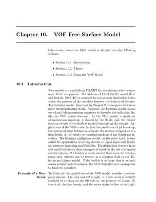
  • 3. 10.1 Introduction 10-3 1.00E+00 5.00E-01 0.00E+00 Y Transient Simulation of a Dam Break Oct 20 1994 Z X Water Volume Fraction (Dim) Fluent 4.30 Lmax = 1.000E+00 Lmin = 0.000E+00 Time = 2.000E-01 Fluent Inc. Figure 10.1.1: Transient Simulation of a Dam Break During the First 0.2 Seconds 1.00E+00 5.00E-01 0.00E+00 Y Transient Simulation of a Dam Break Oct 20 1994 Z X Water Volume Fraction (Dim) Fluent 4.30 Lmax = 1.000E+00 Lmin = 0.000E+00 Time = 7.000E-01 Fluent Inc. Figure 10.1.2: Transient Simulation of a Dam Break at 0.5 and 0.7 Seconds c Fluent Inc. May 10, 1997
  • 4. 10-4 Chapter 10 | VOF Free Surface Model 1.00E+00 5.00E-01 0.00E+00 Y Transient Simulation of a Dam Break Oct 24 1994 Z X Water Volume Fraction (Dim) Fluent 4.30 Lmax = 1.000E+00 Lmin = 0.000E+00 Time = 1.100E+00 Fluent Inc. Figure 10.1.3: Transient Simulation of a Dam Break at 0.9 and 1.1 Seconds Steady State vs. The VOF formulation in FLUENT is, by default, time-dependent, Time Dependence but for problems in which you are concerned only with a steady- state solution, it is possible to perform a steady-state calculation. A steady-state VOF calculation is sensible only when your solution is independent of the initial conditions and there are distinct in ow boundaries for the individual phases. For example, since the shape of the free surface inside a rotating cup depends on the initial level of the uid, such a problem must be solved using the time-dependent formulation. On the other hand, the ow of water in a channel with a region of air on top and a separate air inlet can be solved with the steady-state formulation. c Fluent Inc. May 10, 1997
  • 5. 10.2 Theory 10-5 10.2 Theory The VOF formulation relies on the fact that two or more uids or phases are not interpenetrating. For each additional phase that you add to your model, a variable is introduced, which is the volume fraction of that phase. In each control volume, the volume fractions of all phases add to unity. The elds for all variables and properties are shared by the phases, as long as the volume fraction of each of the phases is known at each location. Thus the variables and properties in any given cell are either purely representative of one of the phases, or are representative of a mixture of the phases, depending upon the volume fraction values. In other words, if the volume fraction of the kth uid in a multi- uid system is denoted k , then the following three conditions are possible: k = 0 the cell is empty of the kth uid k = 1 the cell is full of the kth uid 0 k 1 the cell contains the interface between the uids Based on the local value of k , the appropriate properties and vari- ables will be assigned to each control volume within the domain. The Volume The tracking of the interfaces between the phases is accomplished Fraction Equation by the solution of a continuity equation for the volume fraction of one or more of the phases. For the kth phase, this equation has the form: @ @ @t k + uj @xk = S k 10.2-1 i The source term on the right hand side of Equation 10.2-1 is nor- mally zero, but can be constructed with a User-De ned Subroutine to generate a source of the kth phase in one or more regions of the solution domain to simulate mass transfer between phases. This task requires the additional speci cation of a mass source. Properties The properties appearing in the transport equations are determined by the presence of the component phases in each control volume. In a two-phase system, for example, if the phases are represented by the subscripts 1 and 2, and if the volume fraction of the second of these is being tracked, the density in each cell is given by: = 2 2 + 1 , 2 1 10.2-2 In general, for an N-phase system, the volume-fraction averaged density takes on the form: c Fluent Inc. May 10, 1997
  • 6. 10-6 Chapter 10 | VOF Free Surface Model X = k k 10.2-3 All other properties are computed in this manner viscosity and thermal conductivity, for example with the exception of the speci c heat, which is mass fraction averaged: P k cp k cp = P 10.2-4 k k k The basis for the mass-weighted averaging done for the speci c heat lies in the manner in which the enthalpy is calculated at cells near the interface. The enthalpy in general is dependent upon the ther- mal mass of the uid. It follows, therefore, that a mass-averaged enthalpy be computed at and near interface cells. For cells in this region, the enthalpy at the node P is computed as follows: P k hk hP = Pk 10.2-5 k k The Momentum A single momentum equation is solved throughout the domain, and Equation the resulting velocity eld is shared among the phases. The momen- tum equation, shown below, is dependent on the volume fraction of the kth phase through the properties and . @ @ uj + ui uj @t @xi ! = , @x + @x @P @ @ui @xj + @x + @uj gj + Fj 10.2-6 j i i One limitation of the shared- elds approximation is that in cases where large velocity di erences exist between the phases, the accu- racy of the velocities computed near the interface can be adversely a ected. The Enthalpy The enthalpy equation, also shared between the phases, is shown Equation below. ! @ @ @ @T @t h + @x ui h = @x k @xi + Sh 10.2-7 i i The properties and k are shared by the phases, as discussed earlier. The source term, Sh, contains contributions from radiation, and the c Fluent Inc. May 10, 1997
  • 7. 10.2 Theory 10-7 heat of reaction in the primary phase if reactions are a part of the model. As with the velocity eld, the accuracy of the enthalpy and conse- quently the temperature near the interface is limited in cases where large temperature di erences exist between the phases. Such prob- lems also arise in cases where the properties vary by several orders of magnitude. For example, if a model includes liquid metal in combination with air, the conductivities of the materials can di er by as much as 4 orders of magnitude. Such large discrepancies in properties lead to equation sets with anisotropic coe cients, which in turn lead to convergence and precision limitations. Additional Scalar Depending upon your problem de nition, additional scalar equa- Equations tions may be involved in your solution. In the case of turbulence quantities, a single set of transport equations is solved, and the vari- ables k and are shared by the phases throughout the eld. In the case of species mixing, the species conservation equations are solved throughout the eld, but only pertain to one of the phases. If a cell is completely devoid of that phase, the mass fractions of the rst N-1 species that you name will all take a value of zero in that cell. Interpolation Near The control volume formulation requires that convection and dif- the Interface fusion uxes through the control volume faces be computed and balanced with source terms within the control volume itself. There are two options in FLUENT for the calculation of face uxes for the VOF model. In the default method, which is an explicit approach, the standard interpolation schemes that are used in FLUENT are used to obtain the face uxes whenever a cell is completely lled with one phase or another. When the cell is near the interface between two phases, a donor-acceptor scheme is used to determine the amount of uid advected through the face 49 . This scheme identi es one cell as a donor of an amount of uid from one phase and another neighbor cell as the acceptor of that same amount of uid, and is used to prevent numerical di usion at the interface. The amount of uid from one phase that can be convected across a cell boundary is limited by the minimum of two values: the lled volume in the donor cell or the free volume in the acceptor cell. The orientation of the interface is also used in determining the face uxes. It is determined by the direction of the gradient of the volume fraction of the ith phase within the cell, and that of the neighbor cell which shares the face in question. Depending upon this as well as the motion of the interface, ux values are obtained by c Fluent Inc. May 10, 1997
  • 8. 10-8 Chapter 10 | VOF Free Surface Model pure upwinding, pure downwinding, or some combination of these. In the alternative implicit interpolation method, FLUENT's stan- dard interpolation schemes are used to obtain the face uxes for all cells, including those near the interface. Thus, a standard scalar transport equation is solved for each of the secondary-phase volume fractions. The implicit formulation is valid for both steady-state and time-dependent calculations. See Sections 10.1 and 10.3.2 for more information. Time Dependence The default VOF formulation in FLUENT is time-dependent, so Equation 10.2-1 is solved using an explicit time-marching scheme. Time dependence is automatically enabled as soon as you activate the VOF model. A number of options are available for the control of the time-dependent solution. You may use a single time step for the calculation of all of the transport equations, or you can use an automatic re nement of the time step for the multi-step integration of the volume fraction equation. You may update the volume fraction once for each time step, or once for each iteration within each time step. These options are discussed in more detail in the next section of this chapter. If the explicit donor-acceptor interpolation method is disabled, it is possible to turn o time dependence and perform a steady-state calculation. 10.3 Using the VOF Model 10.3.1 Enabling VOF The VOF model can be enabled in one of two ways. Either you can enter the SETUP1 menu and use the DEFINE-MODELS command from the text interface, or you can open the Models panel using the graphical user interface. Using the When you use the panel, the VOF Free Surface model can be chosen Graphical Interface from among the options in the Model drop-down list under Multi- phase on the right-hand side of the panel. c Fluent Inc. May 10, 1997
  • 9. 10.3 Using the VOF Model 10-9 Note that when you select the VOF model with the default donor- acceptor scheme, the Time Dependent Flow model is activated au- tomatically. If you wish to disable time dependence and perform a steady-state calculation, you will need to rst disable the donor- acceptor scheme, as described in Section 10.3.2. When you click Apply in the Models panel, if you are just beginning the problem setup, you may see the following question, which is needed for the allocation of memory needed for the additional phase. c Fluent Inc. May 10, 1997
  • 10. 10-10 Chapter 10 | VOF Free Surface Model Once you have selected one of the multiphase models, the Multi- phase Parameters... button becomes active, allowing you to specify additional model parameters. In the case of the VOF model, this panel allows you to select the optional Surface Tension and Wall Ad- hesion models, disable the Donor-Acceptor Model, and set some of the time-dependent solution control parameters. c Fluent Inc. May 10, 1997
  • 11. 10.3 Using the VOF Model 10-11 The surface tension and wall-adhesion models and the time-dependence parameters that are relevant to the VOF model are discussed later in this chapter. The use of the implicit interpolation scheme rather than the default donor-acceptor scheme is also discussed later. Using the Text From the text interface, the VOF model can be enabled with the Interface DEFINE-MODELS command in the SETUP1 menu. This command re- sults in a menu where you can choose from among many models that are available in FLUENT. SETUP1 ,! DEFINE-MODELS c Fluent Inc. May 10, 1997
  • 12. 10-12 Chapter 10 | VOF Free Surface Model SETUP1- DM COMMANDS AVAILABLE FROM DEFINE-MODELS: CYLINDRICAL-VELOCITIES HEAT-TRANSFER TURBULENCE RADIATION SPECIES-AND-CHEMISTRY MULTIPLE-PHASES QUIT HELP ENTER HELP COMMAND FOR MORE INFORMATION. DEFINE-MODELS- The option to perform either a VOF or an Eulerian multiphase calculation is enabled with the MULTIPLE-PHASES command. DEFINE-MODELS ,! MULTIPLE-PHASES DEFINE-MODELS- MP MULTIPHASE MODELS SELECT ONLY ONE NO EULERIAN-EULERIAN MULTIPHASE FLOW MODEL NO EULERIAN-EULERIAN GRANULAR FLOW MODEL YES VOF FREE SURFACE MODEL D ACTION TOP,DONE,QUIT,REFRESH After you select one of the multiphase models, a new menu appears in which you can continue the model de nition. If you are just beginning the problem setup, you may rst see the following ques- tion, which is needed for the allocation of memory needed for the additional phase. MULTIPHASE MODEL SELECT ONLY ONE *- ** MEMORY ALLOCATION ** I- NUMBER OF ADDITIONAL PHASES TO BE CONSIDERED I- ++DEFAULT 1++ 1 I- DEFAULT ASSUMED COMMANDS AVAILABLE FROM MULTIPHASE: DEFINE-PHASES MULTIPHASE-OPTIONS QUIT HELP ENTER HELP COMMAND FOR MORE INFORMATION. MULTIPHASE- c Fluent Inc. May 10, 1997
  • 13. 10.3 Using the VOF Model 10-13 The DEFINE-PHASES command is used to specify the number of phases and their names, as described in Section 10.3.3. The MULTIPHASE-OPTIONS command is used to enable the surface ten- sion and wall adhesion models that may be used in conjunction with the VOF calculation, or to disable the donor-acceptor scheme. MULTIPHASE ,! MULTIPHASE-OPTIONS MULTIPHASE- MO VOF OPTIONS YES ENABLE DONOR-ACCEPTOR VOF MODEL NO SURFACE TENSION NO WALL ADHESION D ACTION TOP,DONE,QUIT,REFRESH These options are discussed in Section 10.3.2 and 10.3.9. 10.3.2 Choosing the VOF Formulation The VOF formulations that are available in FLUENT are as follows: time-dependent with the donor-acceptor interpolation scheme default time-dependent with the implicit interpolation scheme steady-state with the implicit interpolation scheme The time-dependent formulation with the donor-acceptor scheme is the default scheme, and it should be used whenever you are inter- ested in the time-accurate transient behavior of the VOF solution. This formulation is activated automatically when you rst enable the VOF model as described in Section 10.3.1. The time-dependent formulation with the implicit interpolation scheme can be used if you are looking for a steady-state solution and you are not interested in the intermediate transient ow behavior, but the nal steady-state solution is dependent on the initial ow con- ditions and or you do not have a distinct in ow boundary for each phase. To use this formulation, turn o the donor-acceptor model as described below. While the implicit time-dependent formulation c Fluent Inc. May 10, 1997
  • 14. 10-14 Chapter 10 | VOF Free Surface Model may converge faster than the donor-acceptor formulation, the in- terface between phases will not be as sharp as that predicted with the donor-acceptor scheme. To reduce this di usivity, it is rec- ommended that you use the QUICK discretization scheme for the volume fraction equations. In addition, you may want to consider turning the donor-acceptor scheme back on after calculating a solu- tion with the implicit scheme, in order to obtain a sharper interface. The steady-state formulation can be used if you are looking for a steady-state solution, you are not interested in the intermedi- ate transient ow behavior, and the nal steady-state solution is not a ected by the initial ow conditions and there is a distinct in ow boundary for each phase. To use this formulation, turn o the donor-acceptor model as described below, and then disable the time-dependent ow model in the Models panel or the EXPERT TIME-DEPENDENCE table. As mentioned above, it is recommended that you use the QUICK discretization scheme for the volume frac- tion equations when you use the implicit interpolation scheme. Examples To help you determine the best formulation to use for your problem, examples which use each of the three formulations are listed below: time-dependent with the donor-acceptor scheme: jet breakup time-dependent with the implicit interpolation scheme: shape of the liquid interface in a centrifuge steady-state with the implicit interpolation scheme: ow around a ship's hull Disabling the In the GUI, you can turn o the donor-acceptor scheme in the Mul- Donor-Acceptor tiphase Parameters panel. Click on the Multiphase Parameters... but- Scheme ton in the Models panel, and then turn o the Donor-Acceptor Model under VOF Free Surface Options: c Fluent Inc. May 10, 1997
  • 15. 10.3 Using the VOF Model 10-15 If a steady-state formulation is desired, you can now turn o the Time Dependent Flow option in the Models panel. When the Donor- Acceptor Model is active, it is not possible to disable time depen- dence. When the donor-acceptor model is not active, FLUENT will solve standard scalar transport equations for the secondary volume frac- tions. c Fluent Inc. May 10, 1997
  • 16. 10-16 Chapter 10 | VOF Free Surface Model In the text interface, you can deactivate the donor-acceptor scheme in the VOF OPTIONS table accessed when you use the MULTIPLE- PHASES command in the DEFINE-MODELS menu to enable the VOF model, as described in Section 10.3.1: VOF OPTIONS NO ENABLE DONOR-ACCEPTOR VOF MODEL NO SURFACE TENSION NO WALL ADHESION ACTION TOP,DONE,QUIT,REFRESH If a steady-state formulation is desired, you can now turn o TIME- DEPENDENCE in the EXPERT menu. When the DONOR-ACCEPTOR VOF MODEL is active, it is not possible to disable time dependence. 10.3.3 De ning the Phases The next step in the problem setup is the naming of the phases. Note that while this step is optional, it can facilitate the subse- quent setup process in that the phases will be identi ed by name rather than by number. To de ne the phases, you can use either the DEFINE-PHASES text command in the SETUP1 menu, or the DEFINE-PHASES command in the MULTIPHASE menu that appears after you use the DEFINE-MODELS MULTIPLE-PHASES text command to enable the VOF model. You will be asked rst for the number of secondary phases in the problem whether or not you were prompted for the number of additional phases to be considered earlier, for memory allocation purposes. You will only be allowed to input the same value as before or a smaller value. A greater number of phases cannot be enabled at this point. If you respond that there is 1 secondary phase, a table will result in which you can input the name of the PRIMARY PHASE and the secondary phase, PHASE 2. SETUP1 ,! DEFINE-PHASES c Fluent Inc. May 10, 1997
  • 17. 10.3 Using the VOF Model 10-17 SETUP1- DP I- NUMBER OF SECONDARY PHASES I- ++DEFAULT 1++ 1 PHASE NAMES NOTE : PHASE NAMES CANNOT CONSIST OF A SINGLE CHARACTER C OR X PHASE 1 PRIMARY PHASE PHASE 2 PHASE 2 ACTION TOP,DONE,QUIT,REFRESH Before you name the phases, it is important to give some thought to which of the uids to identify as the PRIMARY PHASE. If you plan to use the gas law, this model is only available for the primary phase. In the same manner, any species mixing or chemical reac- tions will take place only within the primary phase. It is only this phase that allows for the complete spectrum of property model- ing, including the use of kinetic theory, User-De ned Subroutines, non-Newtonian ow, and composition-dependence. Temperature dependence through polynomial or piecewise-linear pro les, on the other hand, is available for all phases. If your problem de nition does not require the gas law, species mixing, or special property de nitions, you should identify the less dense of the uids as the primary phase. This means that the vol- ume fraction equations will be solved for the denser uids. The motivation for this choice has to do with numerics. If, during the course of the solution, small perturbations in the pressure eld occur near the interface, these will translate into perturbations in the ve- locity eld. Because of the increased inertia, velocity perturbations are smaller and much less destabilizing in the denser uid than in the lighter uid. If the volume fraction is computed for the denser uid, the increased stability of the velocity eld leads to increased stability in the volume fraction calculation. Once you have determined which uid should be assigned to which phase, the phases can be named, as shown below for a two-phase system involving AIR and WATER. c Fluent Inc. May 10, 1997
  • 18. 10-18 Chapter 10 | VOF Free Surface Model PHASE NAMES NOTE : PHASE NAMES CANNOT CONSIST OF A SINGLE CHARACTER C OR X AIR PRIMARY PHASE WATER PHASE 2 D ACTION TOP,DONE,QUIT,REFRESH If you request 2 secondary phases, the table will ask for the names of the primary and the two secondary phases. SETUP1- DP I- NUMBER OF SECONDARY PHASES I- ++DEFAULT 1++ 2 PHASE NAMES NOTE : PHASE NAMES CANNOT CONSIST OF A SINGLE CHARACTER C OR X AIR PRIMARY PHASE WATER PHASE 2 OIL PHASE 3 D ACTION TOP,DONE,QUIT,REFRESH 10.3.4 Time-Dependent Modeling Parameters If you are using the time-dependent VOF formulation in FLUENT, an explicit solution for the volume fraction is obtained either once each time step or once each iteration, depending upon your inputs to the model. You also have control over the time step used for the volume fraction calculation. It can be either the same as that used for the solution of the other transport equations in the model, or it can be adjusted automatically by FLUENT, again based on your inputs. From the text interface, the time-dependent solution controls are accessed from the EXPERT menu using the TIME-DEPENDENCE com- mand. EXPERT ,! TIME-DEPENDENCE c Fluent Inc. May 10, 1997
  • 19. 10.3 Using the VOF Model 10-19 EXPERT- TD TIME DEPENDENT FLOW SOLUTION PARAMETERS 100 MAX. NO. ITNS PER TIME STEP 1.0000E-03 MIN. RESIDUAL SUM DIM 1.0000E-03 SET TIME STEP S YES SOLVE VOF EVERY ITERATION NO AUTOMATIC TIME STEP REFINEMENT FOR VOF 2.5000E-01 MAXIMUM COURANT NUMBER FOR VOF DIM NO AUTOMATIC SAVING NO ENABLE TIME VARYING GRAVITY VECTOR ACTION TOP,DONE,QUIT,REFRESH The input lines in this table are the same as those appearing in the table when the VOF model is not active, with the exception of three. These are discussed below. SOLVE VOF EVERY ITERATION: A response of yes or no to this question allows you to request that FLUENT solve the vol- ume fraction equations every iteration within a time step or simply once a time step. If you solve these equations ev- ery iteration, the convective ux coe cients appearing in the other transport equations will be updated based on the up- dated volume fraction each iteration. If you solve the VOF equations once a time step, these coe cients will not be com- pletely updated each iteration, since the volume fraction eld will not change from iteration to iteration. In general, if you anticipate that the location of the inter- face will change as the other ow variables converge during the time step, you should use a response of YES. This situa- tion arises when large time steps are being used in hopes of reaching a steady-state solution, for example. If small time steps are being used, however, it is not necessary to perform the additional work of solving for the volume fraction every iteration, so an input of NO can be used. This choice is the more stable of the two, and requires less computational e ort per iteration than the rst choice, but the overall result is less accurate in time. AUTOMATIC TIME STEP REFINEMENT FOR VOF: Two options are available for the choice of time step to be used for the volume fraction calculation. If you respond NO to this option, FLU- ENT will solve the VOF equations using the time step that c Fluent Inc. May 10, 1997
  • 20. 10-20 Chapter 10 | VOF Free Surface Model is set in this table on the SET TIME STEP S line. If you re- spond YES, the time step will be re ned automatically, based on your input for the maximum Courant Number allowed near the free surface, discussed below. MAXIMUM COURANT NUMBER FOR VOF DIM: The Courant Num- ber is a dimensionless number that compares the time step in a calculation to the characteristic time of transit of a uid element across a control volume: t 10.3-1 xcell =v uid In the region near the uid interface, FLUENT divides the volume of each cell by the sum of the outgoing uxes. The resulting time represents the time it would take for the uid to empty out of the cell. The smallest such time is used as the characteristic time of transit for a uid element across a control volume, as described above. Based upon this time and your input for the maximum allowed Courant Number, a time step is computed for use in the VOF calculation. For example, if the maximum allowed Courant Number is 0.25, the time step will be chosen to be at most one-fourth the minimum transit time for any cell near the interface. You can access the time-dependent ow parameters from the graph- ical interface, as well. Recall that as soon as the VOF model is enabled in the Models panel, the Time Dependent Flow option is en- abled as well. If you open the Time Dependent Flow Parameters panel from the Models panel, you can set the standard time-dependent ow variables. c Fluent Inc. May 10, 1997
  • 21. 10.3 Using the VOF Model 10-21 To set the time dependent ow parameters that are used in the VOF model, you can use the Multiphase Parameters panel that can be accessed once one of the multiphase models is enabled. c Fluent Inc. May 10, 1997
  • 22. 10-22 Chapter 10 | VOF Free Surface Model In this panel, you can choose whether or not to solve the VOF equations every iteration, whether or not to use the automatic re- nement of the time step, as described above, and set the limiting Courant Number. 10.3.5 De ning the Properties The uid properties are set up using the PHYSICAL-CONSTANTS com- mand in the SETUP1 menu. The items appearing in the PHYSICAL- CONSTANTS menu depend upon the scope of your problem de nition. c Fluent Inc. May 10, 1997
  • 23. 10.3 Using the VOF Model 10-23 At the very least, options for setting the DENSITY and VISCOSITY will appear. Thermal properties appear when temperature is being calculated. Species-related properties appear when the calculation involves two or more species. Kinetic theory parameters appear when kinetic theory is active, and so forth. When the VOF model is active, the same items appear in the menu, but the dialogue that follows when you set the properties changes. This dialogue is de- signed to allow you to set the properties for each of the active phases in your problem. It is illustrated through a number of examples that follow. Setting the Density When the VOF model is active, the gas law can be used for the density calculation for the primary phase only. Alternatively, the phases can have temperature dependent densities. In the simplest case, the phases have constant, but di erent densities. If such a system consists of two phases, the following dialogue illustrates the setup of constant densities. SETUP1 ,! PHYSICAL-CONSTANTS ,! DENSITY c Fluent Inc. May 10, 1997
  • 24. 10-24 Chapter 10 | VOF Free Surface Model SETUP1- PC COMMANDS AVAILABLE FROM PHYSICAL-CONSTANTS: DENSITY VISCOSITY OPERATING-PRESSURE QUIT HELP ENTER HELP COMMAND FOR MORE INFORMATION. PHYSICAL-CONSTANTS- DE COMMANDS AVAILABLE FROM PHASE-SELECTION: AIR WATER QUIT HELP ENTER HELP COMMAND FOR MORE INFORMATION. PHASE-SELECTION- AIR L- USE GAS LAW FOR AIR? L- Y OR N ++DEFAULT-NO++ N R- DENSITY OF AIR R- UNITS= KG M3 ++DEFAULT 1.0000E+03++ 1.0 COMMANDS AVAILABLE FROM PHASE-SELECTION: AIR WATER QUIT HELP ENTER HELP COMMAND FOR MORE INFORMATION. PHASE-SELECTION- WAT R- DENSITY OF WATER R- UNITS= KG M3 ++DEFAULT 1.2930E+00++ 1000 PHASE-SELECTION- Q In the next example, consider a 3-phase system where the gas law is to be used for the primary phase. As with any single phase system involving a single species, FLUENT will ask for the molecular weight for the material being modeled with the gas law. c Fluent Inc. May 10, 1997
  • 25. 10.3 Using the VOF Model 10-25 PHYSICAL-CONSTANTS- DE COMMANDS AVAILABLE FROM PHASE-SELECTION: AIR WATER QUIT HELP ENTER HELP COMMAND FOR MORE INFORMATION. PHASE-SELECTION- AIR L- USE GAS LAW FOR AIR? L- Y OR N ++DEFAULT-NO++ Y R- OPERATING PRESSURE R- UNITS= PA ++DEFAULT 1.0132E+05++ X R- DEFAULT ASSUMED R- ENTER THE MOLECULAR WEIGHT FOR AIR R- UNITS= DIM ++DEFAULT 2.8970E+01++ X R- DEFAULT ASSUMED PHASE-SELECTION- WAT R- DENSITY OF WATER R- UNITS= KG M3 ++DEFAULT 1.2930E+00++ 1000 PHASE-SELECTION- Q If you are modeling multiple species in the primary phase, you will not be asked to input the molecular weight, but will be re- minded to input molecular weights for all of the species using the MOLECULAR-WEIGHTS command. When you are solving for temperature, FLUENT asks for the tem- perature dependence for all of the properties for all of the phases. For example, for a 3-phase system, the dialogue for setting up the densities would be similar to that shown below. c Fluent Inc. May 10, 1997
  • 26. 10-26 Chapter 10 | VOF Free Surface Model PHYSICAL-CONSTANTS- DE COMMANDS AVAILABLE FROM PHASE-SELECTION: AIR OIL WATER QUIT HELP ENTER HELP COMMAND FOR MORE INFORMATION. PHASE-SELECTION- AIR L- USE GAS LAW FOR AIR? L- Y OR N ++DEFAULT-NO++ Y R- OPERATING PRESSURE R- UNITS= PA ++DEFAULT 1.0132E+05++ X R- DEFAULT ASSUMED R- ENTER THE MOLECULAR WEIGHT FOR AIR R- UNITS= DIM ++DEFAULT 2.8970E+01++ X R- DEFAULT ASSUMED PHASE-SELECTION- WAT *- DEFINE DENSITY OF WATER KG M3 *- AS A FUNCTION OF TEMPERATURE K *- I- NUMBER OF COEFFICIENTS +VE = POLYNOM., -VE = P.W.LINEAR I- ++DEFAULT 1++ 1 R- DENSITY OF WATER KG M3 R- UNITS= KG M3 ++DEFAULT 1.0000E+03++ X R- DEFAULT ASSUMED c Fluent Inc. May 10, 1997
  • 27. 10.3 Using the VOF Model 10-27 PHASE-SELECTION- OIL *- DEFINE DENSITY OF OIL KG M3 *- AS A FUNCTION OF TEMPERATURE K *- I- NUMBER OF COEFFICIENTS +VE = POLYNOM., -VE = P.W.LINEAR I- ++DEFAULT 1++ 2 POLYNOMIAL FIT FOR DENSITY OF OIL 8.0000E+02 ENTER COEFFICIENT - A1 KG M3 -1.0000E-02 ENTER COEFFICIENT - A2 - D ACTION TOP,DONE,QUIT,REFRESH Setting the The viscosities for the phases are input in the same manner. In an Viscosity isothermal, 3-phase system, the viscosities would be input in the manner shown below. PHYSICAL-CONSTANTS ,! VISCOSITY PHYSICAL-CONSTANTS- VI PHASE-SELECTION- AIR R- VISCOSITY OF AIR R- UNITS= KG M-S ++DEFAULT 2.0000E-05++ 1.7e-5 PHASE-SELECTION- WAT R- VISCOSITY OF WATER R- UNITS= KG M-S ++DEFAULT 9.0000E-04++ X R- DEFAULT ASSUMED PHASE-SELECTION- OIL R- VISCOSITY OF OIL R- UNITS= KG M-S ++DEFAULT 1.7200E-05++ .01 If you are calculating temperature, FLUENT will ask for the tem- perature dependence of the viscosity for each phase, in the manner shown above for the density. c Fluent Inc. May 10, 1997
  • 28. 10-28 Chapter 10 | VOF Free Surface Model Modeling a In the event that one of the phases is to be modeled as a non- Non-Newtonian Newtonian uid, you must de ne this uid as the primary phase. Viscosity Once the non-Newtonian model has been enabled in the EXPERT OPTIONS table or the Models panel, the VISCOSITY command in the PHYSICAL-CONSTANTS menu can be used to set the non-Newtonian viscosity constants as well as the viscosity for the additional phases. SETUP1- PC COMMANDS AVAILABLE FROM PHYSICAL-CONSTANTS: DENSITY VISCOSITY PROPERTY-OPTIONS OPERATING-PRESSURE QUIT HELP ENTER HELP COMMAND FOR MORE INFORMATION. PHYSICAL-CONSTANTS- VIS PHASE-SELECTION- AIR NON-NEWTONIAN FLOW PARAMETERS POWER LAW FOR AIR 1.5 PARAMETER N DIM 1.0000E+00 PARAMETER K PA*S**N D ACTION TOP,DONE,QUIT,REFRESH PHASE-SELECTION- WAT R- VISCOSITY OF WATER R- UNITS= KG M-S ++DEFAULT 1.7200E-05++ 9E-4 Using Kinetic If you are using the gas law to model the primary phase, you will Theory for have the option of using kinetic theory to model one or more of Property De nition the other properties for that phase. The kinetic theory option is enabled in the usual way, using the PROPERTY-OPTIONS table in the PHYSICAL-CONSTANTS menu. Once enabled, you will be asked if you want to use kinetic theory when you set the various properties. For example, to use kinetic theory for the speci c heat, the dia- logue would proceed as shown below. After setting the REFERENCE TEMPERATURE FOR ENTHALPY and selecting the primary phase AIR in the example below, you will be asked if you want to use kinetic theory for the primary phase: c Fluent Inc. May 10, 1997
  • 29. 10.3 Using the VOF Model 10-29 PHYSICAL-CONSTANTS- CP R- REFERENCE TEMPERATURE FOR ENTHALPY R- UNITS= K ++DEFAULT 2.7300E+02++ X R- DEFAULT ASSUMED PHASE-SELECTION- AIR L- COMPUTE SPECIFIC HEAT FROM KINETIC THEORY? L- Y OR N ++DEFAULT-YES++ Y You can then de ne the optionally temperature-dependent speci c heat for the remaining phases. PHASE-SELECTION- WAT *- DEFINE SPECIFIC HEAT OF WATER J KG-K *- AS A FUNCTION OF TEMPERATURE K *- I- NUMBER OF COEFFICIENTS +VE = POLYNOM., -VE = P.W.LINEAR I- ++DEFAULT 1++ X I- DEFAULT ASSUMED R- SPECIFIC HEAT OF WATER J KG-K R- UNITS= J KG-K ++DEFAULT 1.0000E+03++ 4136 Before kinetic theory can be used, you will need to set the kinetic theory parameters, appearing in the KINETIC-THEORY-PARMS. ta- ble. The setting of these parameters is described in Chapter 15. 10.3.6 Including Body Forces in the VOF Calculation In many instances, the motion of the uids you are tracking with the VOF model is due, in part, to gravitational e ects. When you ac- tivate a gravitational force in the BODY-FORCES table in the EXPERT menu, you will be given a choice of whether to set the site of the reference density or to set the reference density itself. EXPERT ,! BODY-FORCES c Fluent Inc. May 10, 1997
  • 30. 10-30 Chapter 10 | VOF Free Surface Model SETUP1- EX BF BODY FORCES YES IMPROVED TREATMENT OF BODY FORCE IN DISCRETE EQNS. YES INCLUDE BODY FORCE TERMS IN VELOCITY INTERPOLATION 9.8000E+00 GRAVITY ACCELERATION IN X-DIRN - M S2 0.0000E+00 GRAVITY ACCELERATION IN Y-DIRN - M S2 YES USER DEFINED REFERENCE DENSITY D ACTION TOP,DONE,QUIT,REFRESH If you respond YES to the option to input a USER DEFINED REFERENCE DENSITY, a second table will appear, where you will be able to input the value of this density. USER DEFINED REFERENCE DENSITY 1.0000E+00 REFERENCE DENSITY KG M3 D ACTION TOP,DONE,QUIT,REFRESH If you respond NO to the input of a USER DEFINED REFERENCE DENSITY, a second table will appear asking you to input the location of the cell from which the reference density will be taken. REFERENCE DENSITY LOCATION 2 REFERENCE DENSITY : I - LOCATION 2 REFERENCE DENSITY : J - LOCATION ACTION TOP,DONE,QUIT,REFRESH While either selection works well for most single phase applications, the option to set the reference density rather than the site of the reference density is preferred when the VOF model is in use. The aim is to have a reference density value that is stable throughout the calculation. Since many VOF applications involve a change from one phase to another in any given control volume throughout the course of the calculation, it is better to set the density value itself, rather than assume that one cell in particular will always be lled with one particular phase. In terms of selecting the appropriate reference density value, the best strategy is to use the density of the predominant uid. If, in a two-phase system, for example, water occupies over 50 of c Fluent Inc. May 10, 1997
  • 31. 10.3 Using the VOF Model 10-31 the volume, the density of water should be used. This strategy minimizes the round-o in the density uctuations that are the source of the buoyancy forces in the domain. If your model has in ow out ow boundaries and you prefer to set the reference density site, you should do so at an in ow boundary where the predominant uid enters the domain. This is because the density will be constant throughout the calculation at this site. If you choose an interior site, convergence problems will arise if uctuations of the density occur at the site that you choose. 10.3.7 Setting Boundary Conditions Boundary conditions may be input using either the text interface command for BOUNDARY-CONDITIONS in the SETUP1 menu, or the Boundary Conditions panel through the graphical user interface. At inlets, one additional scalar, the volume fraction, must be set when the VOF model is active. Note that this scalar can only be set for the non-primary phases. In a 2-phase system, for example, where the primary phase is air and the second phase is water, the steps for setting the inlet boundary conditions from the graphical user interface are as follows. From the Boundary Conditions panel, choose an INLET cell type and select the appropriate zone ID. When you press the Set... button the Velocity or Pressure Inlet Boundary Conditions panel appears. c Fluent Inc. May 10, 1997
  • 32. 10-32 Chapter 10 | VOF Free Surface Model In the Inlet Boundary Conditions panel, the rst Phase that you named appears in the upper left corner, and the elds for the rel- evant velocities and scalars are active. The Volume Fraction eld under Multiphase is not active at this time. The speci cation of the boundary conditions requires two steps. First, enter the velocity and other scalar values in the appropriate elds and click on Apply. Second, choose one of the secondary phases from the Phase drop-down list. When you do this, the velocity and c Fluent Inc. May 10, 1997
  • 33. 10.3 Using the VOF Model 10-33 scalar elds become inactive, and the Volume Fraction eld becomes active. Set the appropriate Volume Fraction and click on Apply. If, in a two-phase system, the inlet is to have a volume fraction of 1 for the rst phase, you will need to choose the second phase and set a volume fraction of 0. Note that with the VOF Model, only values of 0 or 1 are meaningful at any given inlet. If an inlet is to introduce a strati ed layer of two uids into a domain, it should be replaced by two inlets, each carrying a single uid. c Fluent Inc. May 10, 1997
  • 34. 10-34 Chapter 10 | VOF Free Surface Model From the text interface, the VOLUME-FRACTION appears in the inlet zone boundary conditions menu as shown below. SETUP1 ,! BOUNDARY-CONDITIONS SETUP1- BC COMMANDS AVAILABLE FROM BOUNDS: W-WALL Z-WALL SYMMETRY .LIVE CYCLIC OUTLET INLET AXIS QUIT HELP ENTER HELP COMMAND FOR MORE INFORMATION. BOUNDS- I 1 COMMANDS AVAILABLE FROM I1-ZONE-BOUNDARY-CONDITIONS: NORMAL-VELOCITY U-VELOCITY V-VELOCITY VOLUME-FRACTION QUIT HELP ENTER HELP COMMAND FOR MORE INFORMATION. I1-ZONE-BOUNDARY-CONDITIONS- As with the graphical interface, the VOLUME-FRACTION command will prompt you for the volume fraction of the secondary phases only. Thus, if you are solving a problem in which there is one sec- ondary phase, FLUENT will ask for the volume fraction of only that phase. Volume fractions of either 0 or 1.0 are the only meaningful choices for the VOF model, even though any value between these two will be accepted. BOUNDARY-CONDITIONS ,! VOLUME-FRACTION I1-ZONE-BOUNDARY-CONDITIONS- VF R- VOLUME FRACTION OF WATER R- UNITS= DIM ++DEFAULT 0.0000E+00++ 1.0 Because the velocity and turbulence and enthalpy elds are shared, there is no need to specify a separate velocity boundary condition for the various phases. This is in contrast to the setting of bound- ary conditions in the Eulerian multiphase model, where each phase c Fluent Inc. May 10, 1997
  • 35. 10.3 Using the VOF Model 10-35 carries its own velocity eld. Wall boundary condition options are not expanded by the presence of multiple phases within the domain. A zero normal gradient boundary condition is imposed for the volume fraction. 10.3.8 Solution Strategies In addition to the appropriate choice for the primary phase uid and the time stepping technique to use, other steps can be taken to improve the accuracy of the VOF calculation. Setting the The site of the reference pressure can be moved to a location that Reference Pressure will result in less round-o in the pressure calculation. The option Location to set the reference pressure location is in the EXPERT SOLUTION- PARAMETERS table. If you respond YES, as shown below, a second table appears in which the location of the reference pressure can be chosen. EXPERT ,! SOLUTION-PARAMETERS SOLUTION PARAMETERS NO MONITOR SOLVER NO ALLOW PATCHING OF BOUNDARY VALUES YES CONVERGENCE-DIVERGENCE CHECK ON 1.0000E-03 SET MINIMUM RESIDUAL SUM DIM YES NORMALIZE RESIDUALS YES CONTINUITY CHECK NO ENABLE HIGHER ORDER SCHEME NO ENABLE LINEAR INTERPOLATION FOR PRESSURE NO VISCOSITY WEIGHTED VELOCITY INTERPOLATION NO ENABLE SIMPLEC METHOD DEFAULT IS SIMPLE NO ENABLE FIX VARIABLE OPTION YES SET PRESSURE REFERENCE LOCATION D ACTION TOP,DONE,QUIT,REFRESH REFERENCE PRESSURE LOCATION 2 I-VALUE 10 J-VALUE D ACTION TOP,DONE,QUIT,REFRESH The cell that you choose should be in a region that will always contain the less dense of the two uids. This is because variations in the static pressure are larger in a more dense uid than in a less dense uid, given the same velocity distribution. If the zero of the relative pressure eld is in a region where the pressure variations are c Fluent Inc. May 10, 1997
  • 36. 10-36 Chapter 10 | VOF Free Surface Model small, less round-o will occur than if the variations occur in a eld of large non-zero values. Thus in systems containing air and water, for example, it is important that the reference pressure location be in the portion of the domain lled with air rather than that lled with water. Setting the The calculation of pressure is perhaps the most important among all Multigrid of the variables in a VOF simulation in terms of having an in uence Parameters on the prediction of volume fraction. Whenever possible, the multi- grid solver should be enabled for pressure. To extract the most work from the multigrid solver each iteration, you should decrease the TERMINATION-CRITERIA to its minimum value, 1 10,3 , at least during the rst few time steps, using the TERMINATION-CRITERIA command in the MULTIGRID-PARAMETERS menu or the Termination Criterion eld in the Multigrid Parameters panel. EXPERT ,! LINEAR-EQN.-SOLVERS ,! MULTIGRID-PARAMETERS Solve ,! Controls ,!Multigrid... Reduction of this value leads to the maximum volume conservation condition that can be imposed during each iteration, leading to the most accurate prediction of the volume fraction. Underrelaxation A third change that you may want to make to the solver settings is for the in the underrelaxation factors that you use. Typically, the default Time-Dependent time-dependent VOF formulation allows for increased values on all Donor-Acceptor underrelaxation factors, provided a small time step is used, without Formulation a loss of solution stability. In simple geometries with little grid skew, you can generally increase the underrelaxation factors for all variables to 1.0 and expect stability and a rapid rate of convergence in the form of few iterations required per time step. The default underrelaxation factor of 1.0 on the body forces need not be reduced except in cases where gravity and strong swirl or other user-de ned momentum sources are involved. EXPERT ,! UNDERRELAX1 Solve ,! Controls ,!Underrelaxation... As with any FLUENT simulation, the underrelaxation factors can and should be increased as the solution exhibits stable, convergent behavior. You should always save a Data File beforehand, however, in case the increase you specify destabilizes the solution process. Underrelaxation If you have deactivated the donor-acceptor model as described in for the Implicit Section 10.3.2, you will be able to set underrelaxation parame- Formulations ters for each secondary-phase volume-fraction transport equation. c Fluent Inc. May 10, 1997
  • 37. 10.3 Using the VOF Model 10-37 This is true for both the time-dependent and steady-state implicit formulations. By default, these underrelaxation factors are set to 0.2. For improved convergence, you can set these as well as the underrelaxation factors for all other equations to 0.5. Linear Solver As mentioned earlier, if you have deactivated the donor-acceptor Parameters for the model as described in Section 10.3.2, FLUENT will solve trans- Implicit port equations for the secondary-phase volume fractions. It is not Formulations possible to use the multigrid solver for these volume fraction equa- tions, so you must always use the linear LGS solver. Discretization When the implicit scheme is used instead of the donor-acceptor Scheme Selection scheme, you should use the QUICK discretization scheme for the for the Implicit volume fraction equations in order to improve the sharpness of the Formulations interface between phases. 10.3.9 The Surface Tension Model It is possible to include the e ects of surface tension along the in- terface between two uids. The model can be augmented by the additional speci cation of a contact angle that one of the uids makes with the container wall. Surface tension arises as a result of attractive forces between molecules in a uid. Consider an air bubble in water, for example. Within the bubble, the net force on a molecule due to its neighbors is zero. At the surface, however, the net force is radially inward, and the combined e ect of the radial components of force across the entire spherical surface is to make the surface contract, thereby increasing the pressure on the concave side of the surface. The surface tension is a force, acting only at the surface, that is required to maintain equilibrium in such instances. It acts to balance the radially inward inter-molecular attractive force with the radially outward pressure gradient force across the surface. In regions where two uids are separated, but one of them is not in the form of spherical bubbles, the surface tension acts to decrease the area of the interface. The surface tension model in FLUENT is the Continuum Surface Force CSF model proposed by Brackbill et al. 14 . With this model, the addition of surface tension to the VOF calculation results in a source term to the momentum equation. To understand the origin of the source term, consider the special case where the surface tension is constant along the surface, and where only the forces normal to the interface are considered. It can be shown that the pressure drop across the surface depends upon the surface tension coe cient, , and the surface curvature as measured by two radii c Fluent Inc. May 10, 1997
  • 38. 10-38 Chapter 10 | VOF Free Surface Model in orthogonal directions, R1 and R2:
  • 39. 1 1 p2 , p1 = R1 +R 10.3-2 2 where p1 and p2 are the pressures in the two uids on either side of the interface. In FLUENT, a more general formulation is used, where the surface curvature is computed from local gradients in the surface normal at the interface. Let n be the surface normal, de ned as the gradient in 2 , the secondary phase volume fraction. n =r 2 10.3-3 The curvature, , is de ned in terms of the divergence of the unit normal, n: ^ ! =rn = 1 jnj r jnj , r n n ^ jnj 10.3-4 where n ^ = jnj n 10.3-5 The surface tension can be written in terms of the pressure jump across the surface. The force at the surface can be expressed as a volume force using the divergence theorem. It is this volume force that is the source term which is added to the momentum equation. It has the following form: = 2 x 2 r 2 Fvol x 10.3-6 Note that the source term is only added on one side of the inter- face: the side on which the volume fraction calculation is being performed. In the FLUENT VOF model, this corresponds to the secondary phase. Example: As an example of the surface tension model, consider a section of a Prediction of a stationary cylinder of water in a zero gravitational eld. The sec- Capillary Jet tion is 5.236 cm in length, and roughly 1 cm in diameter, following Breakup an example proposed in Reference 65 . A region of air, 3 cm in diameter, surrounds the cylinder of water. A 41 31 grid is used c Fluent Inc. May 10, 1997
  • 40. 10.3 Using the VOF Model 10-39 in the axisymmetric model, which employs a symmetry boundary condition on the axis and both ends, and a pressure boundary to model the plenum of air surrounding the water. The liquid surface is initially perturbed at t=0 so that the diameter at the left side is 5 larger than that at the right Figure 10.3.1, with the transition modeled using a cosine function. 1.00E+00 5.00E-01 0.00E+00 Y Initial Conditions for Capillary Jet Breakup Nov 03 1994 Z X Water Volume Fraction (Dim) Fluent 4.30 Max = 1.000E+00 Min = 0.000E+00 Time = 5.000E-04 Fluent Inc. Figure 10.3.1: Initial Conditions for Capillary Jet Breakup Problem As time evolves, the perturbation in the surface grows, as can be seen in Figure 10.3.2. The reason that the perturbation grows in this manner is that the curvature in the surface gives rise to di erent pressure gradients across the surface in di erent regions. Where the surface is concave as seen from the water side, the pressure is higher on the water side than on the air side, forcing the boundary to move outward. Where the surface is convex, the opposite is true, so that the boundary moves inward. At t = 0.75 seconds Figure 10.3.3, the perturbation has advanced to the point where the jet is about to break. Within the next 15 ms, the break up has occurred. Enabling the The surface tension model can be enabled three di erent ways. Surface Tension First, you can open the Multiphase Parameters panel and turn on Model the Surface Tension check button. c Fluent Inc. May 10, 1997
  • 41. 10-40 Chapter 10 | VOF Free Surface Model 1.00E+00 5.00E-01 0.00E+00 Y Capillary Jet Breakup at t = 0.5 / 0.7 sec Nov 03 1994 Z X Water Volume Fraction (Dim) Fluent 4.30 Max = 1.000E+00 Min = 0.000E+00 Time = 7.000E-01 Fluent Inc. Figure 10.3.2: Capillary Jet Breakup at T = 0.5 top and 0.7 bottom sec c Fluent Inc. May 10, 1997
  • 42. 10.3 Using the VOF Model 10-41 1.00E+00 5.00E-01 0.00E+00 Y Capillary Jet Breakup at t = 0.75 / 0.765 sec Nov 03 1994 Z X Water Volume Fraction (Dim) Fluent 4.30 Max = 1.000E+00 Min = 0.000E+00 Time = 7.650E-01 Fluent Inc. Figure 10.3.3: Capillary Jet Breakup at T = 0.75 top and 0.765 bottom sec c Fluent Inc. May 10, 1997
  • 43. 10-42 Chapter 10 | VOF Free Surface Model Alternatively, you can use the text interface. In the SETUP1 menu, you can start with the DEFINE-MODELS command and select the MULTIPLE-PHASES option to turn on the VOF FREE SURFACE MODEL. DEFINE-MODELS- MP MULTIPHASE MODELS SELECT ONLY ONE NO EULERIAN-EULERIAN MULTIPHASE FLOW MODEL NO EULERIAN-EULERIAN GRANULAR FLOW MODEL YES VOF FREE SURFACE MODEL D ACTION TOP,DONE,QUIT,REFRESH After you select one of the multiphase models, a new menu ap- pears in which you can name the phases, as described earlier, or choose MULTIPHASE-OPTIONS that are relevant to the VOF model: the SURFACE TENSION model with the optional addition of WALL ADHESION described later in this section. COMMANDS AVAILABLE FROM MULTIPHASE: DEFINE-PHASES MULTIPHASE-OPTIONS QUIT HELP ENTER HELP COMMAND FOR MORE INFORMATION. MULTIPHASE- MO VOF OPTIONS YES ENABLE DONOR-ACCEPTOR VOF MODEL YES SURFACE TENSION NO WALL ADHESION D ACTION TOP,DONE,QUIT,REFRESH Finally, you can use the OPTIONS command in the EXPERT menu. EXPERT ,! OPTIONS c Fluent Inc. May 10, 1997
  • 44. 10.3 Using the VOF Model 10-43 EXPERT- OP MODELING OPTIONS NO ALLOW LINK SETTING NO ALLOW PROFILE SETTING NO ENABLE NON-NEWTONIAN FLOW MODEL NO ENABLE POROUS FLOW MODEL NO ENABLE FAN RADIATOR MODEL NO ALLOW FIXED PRESSURE BOUNDARIES NO ALLOW SETTING FLOW ANGLES FOR PRESSURE-INLETS NO ENABLE STEADY CORIOLIS FORCE NO ENABLE TIME-DEPENDENT CORIOLIS FORCE NO ENABLE MULTIPLE ROTATING REFERENCE FRAMES YES ENABLE DONOR-ACCEPTOR VOF MODEL YES SURFACE TENSION NO WALL ADHESION NO ENABLE SLIDING MESH CALCULATION NO ACTIVATE PHASE CHANGE MODELING NO ENABLE DEFORMING MESH CALCULATION D ACTION TOP,DONE,QUIT,REFRESH The setting of the surface tension coe cient is illustrated along with the setting of the contact angle that the uid makes with the wall. This so-called wall adhesion angle is discussed below. Wall Adhesion An option to specify a wall adhesion angle in conjunction with the surface tension model is also available in the VOF model. The model is taken from work done by Brackbill et al. 14 . Rather than impose this boundary condition at the wall itself, the contact angle that the uid is assumed to make with the wall is used to adjust the surface normal in cells near the wall. This so-called dynamic boundary condition results in the adjustment of the curvature of the surface near the wall. If
  • 45. w is the contact angle at the wall, then the surface normal at the live cell next to the wall is n ^ ^ ^ = nw cos
  • 46. w + tw sin
  • 47. w 10.3-7 ^ where nw and tw are the unit vectors normal and tangential to ^ the wall, respectively. The combination of this contact angle with the normally calculated surface normal one cell away from the wall determine the local curvature of the surface, and this curvature is used to adjust the body force term in the surface tension calculation. c Fluent Inc. May 10, 1997
  • 48. 10-44 Chapter 10 | VOF Free Surface Model Enabling the Wall The ability to set the contact angle that the uid makes with the Adhesion Model wall is set using one of the three methods discussed earlier for en- abling surface tension. You can use the Multiphase Parameters panel, the MULTIPHASE-OPTIONS menu command, or the EXPERT OPTIONS table. Example: As an example, consider a cylindrical container, partially lled with Formation of a water, in a zero gravity eld. The container is 10 cm tall and 10 Water Bubble cm in diameter. An axisymmetric model is solved using a 51 31 grid. At time t=0, the water lls the bottom 2 cm of the container, with air above it Figure 10.3.4, left frame. The air is modeled as the primary phase, which means that the surface tension value 0.07 N m will be applied to the second phase, water. A contact angle of 175 is used. This contact angle is applied to the water, which means that an obtuse angle, as measured in the water, will form at the walls. For this condition to be met, the water level must rise in the middle of the container and drop at the edges. The start of this process is shown in Figure 10.3.4 right frame, where the boundary condition at the wall acts to change the water level nearby. Note that the water level at the center of the vessel is not yet a ected at this time. After 0.7 sec have passed Figure 10.3.5 left frame, the uid in the center of the container has responded, and the water at the edges continues to try to satisfy the contact angle boundary condition. By 1.3 sec Figure 10.3.5 right frame, the water has become detached from the bottom of the vessel and is moving slowly upward. Setting the Surface The surface tension coe cient and contact angle at the wall are set Tension and Wall in the PHYSICAL-CONSTANTS menu, using the VOF-SURFACE-TENSION Adhesion command. Note that you can specify the surface tension coe cient Properties for only one phase. The contact angle is that between the inter- face and the wall as measured inside the speci ed phase uid. In the example below, a contact angle of 45 corresponds to the water creeping up the side of its container, as is common with water in a glass. SETUP1 ,! PHYSICAL-CONSTANTS ,! VOF-SURFACE-TENSION c Fluent Inc. May 10, 1997
  • 49. 10.3 Using the VOF Model 10-45 1.00E+00 5.00E-01 0.00E+00 Formation of a Bubble in a Zero Gravity Field Oct 21 1994 Z Y Water Volume Fraction (Dim) Fluent 4.30 X Max = 1.000E+00 Min = 0.000E+00 Time = 2.000E-01 Fluent Inc. Figure 10.3.4: Initial Water Level in a Container Left and Altered Water Level After 0.2 sec Right c Fluent Inc. May 10, 1997
  • 50. 10-46 Chapter 10 | VOF Free Surface Model 1.00E+00 5.00E-01 0.00E+00 Formation of a Bubble in a Zero Gravity Field Oct 21 1994 Z Y Water Volume Fraction (Dim) Fluent 4.30 X Max = 1.000E+00 Min = 0.000E+00 Time = 1.300E+00 Fluent Inc. Figure 10.3.5: Formation of a Water Bubble Before Left and After Right it Separates from the Wall c Fluent Inc. May 10, 1997
  • 51. 10.3 Using the VOF Model 10-47 SETUP1- PC COMMANDS AVAILABLE FROM PHYSICAL-CONSTANTS: DENSITY VISCOSITY PROPERTY-OPTIONS OPERATING-PRESSURE VOF-SURFACE-TENSION QUIT HELP ENTER HELP COMMAND FOR MORE INFORMATION. PHYSICAL-CONSTANTS- VOF *- SELECT PHASE FOR SURFACE TENSION *- DEFAULT PHASE - WATER COMMANDS AVAILABLE FROM PHASE-SELECTION: AIR WATER QUIT HELP ENTER HELP COMMAND FOR MORE INFORMATION. PHASE-SELECTION- WAT R- ENTER SURFACE TENSION COEFFICIENT FOR WATER R- UNITS= N M ++DEFAULT 7.3050E-02++ X R- DEFAULT ASSUMED R- ENTER CONTACT ANGLE IN DEGREES R- UNITS= DIM ++DEFAULT 9.0000E+01++ 45 R- DEFAULT ASSUMED The default setting for surface tension coe cient corresponds to water at room temperature and atmospheric pressure. The contact angle is the angle between each boundary wall and the uid interface as measured in the speci ed phase here, water. The default value 90 corresponds to a surface which is at all times normal to the surrounding walls. 10.3.10 Using the VOF Model with Porous Media The VOF model is compatible with the porous media model in FLUENT. If you have a region that needs to be described as a porous media, the setup begins in the normal way. First, you need to enable the porous media model in the EXPERT OPTIONS table in the text c Fluent Inc. May 10, 1997
  • 52. 10-48 Chapter 10 | VOF Free Surface Model interface. The next step is to set the cell types appropriately so as to belong to one or more porous zones. When you set the porous media constants from the PHYSICAL-CONSTANTS menu, FLUENT will prompt you for the PERMEABILITY and INERTIAL- RESISTANCE-FACTOR for each of the phases separately. PHYSICAL-CONSTANTS ,! POROUS-MEDIA PHYSICAL-CONSTANTS- PM *- POROUS MEDIA INPUTS... *- ENTER QUIT WHEN FINISHED SELECT-ZONE- 1 COMMANDS AVAILABLE FROM * POROUS MEDIA INPUTS FOR ZONE 1 *: PERMEABILITY INERTIAL-RESISTANCE-FACTOR POROSITY QUIT HELP ENTER HELP COMMAND FOR MORE INFORMATION. * POROUS MEDIA INPUTS FOR ZONE 1 *- PER PERMEABILITY FOR ZONE 1 1.0000E-08 PERMEABILITY IN THE I-DIRN. FOR PHASE 1 M2 1.0000E-08 PERMEABILITY IN THE J-DIRN. FOR PHASE 1 M2 5.0000E-09 PERMEABILITY IN THE I-DIRN. FOR PHASE 2 M2 5.0000E-09 PERMEABILITY IN THE J-DIRN. FOR PHASE 2 M2 D ACTION TOP,DONE,QUIT,REFRESH * POROUS MEDIA INPUTS FOR ZONE 1 *- IRF INERTIAL RESISTANCE FACTOR FOR ZONE 1 4.0000E+02 INERTIAL FACTOR IN THE I-DIRN. FOR PHASE 1 M 4.0000E+02 INERTIAL FACTOR IN THE J-DIRN. FOR PHASE 1 M 1.0000E+02 INERTIAL FACTOR IN THE I-DIRN. FOR PHASE 2 M 1.0000E+02 INERTIAL FACTOR IN THE J-DIRN. FOR PHASE 2 M NO INERTIAL TERM =C2*DEN*Vi*ABSVi 2 ELSE =C2*DEN*Vi*Vmag 2 D ACTION TOP,DONE,QUIT,REFRESH c Fluent Inc. May 10, 1997
  • 53. 10.3 Using the VOF Model 10-49 Example As an example, consider a long narrow channel that is completely lled with a porous material. CELL TYPES: J I= 2 4 6 8 10 12 14 16 18 20 10 W1W1W1W1W1W1W1W1W1W1W1W1W1W1W1W1W1W1W1W1 10 9 I1*1*1*1*1*1*1*1*1*1*1*1*1*1*1*1*1*1*1I2 9 8 I1*1*1*1*1*1*1*1*1*1*1*1*1*1*1*1*1*1*1I2 8 7 I1*1*1*1*1*1*1*1*1*1*1*1*1*1*1*1*1*1*1I2 7 6 I1*1*1*1*1*1*1*1*1*1*1*1*1*1*1*1*1*1*1I2 6 5 I1*1*1*1*1*1*1*1*1*1*1*1*1*1*1*1*1*1*1I2 5 4 I1*1*1*1*1*1*1*1*1*1*1*1*1*1*1*1*1*1*1I2 4 3 I1*1*1*1*1*1*1*1*1*1*1*1*1*1*1*1*1*1*1I2 3 2 I1*1*1*1*1*1*1*1*1*1*1*1*1*1*1*1*1*1*1I2 2 1 W1W1W1W1W1W1W1W1W1W1W1W1W1W1W1W1W1W1W1W1 1 J I= 2 4 6 8 10 12 14 16 18 20 The duct is initially lled with oil with a density of 800 kg m3 and a viscosity of 0.01 kg m-sec. At t=0, water is allowed to enter the domain from the left under the action of a total pressure of 104 Pascals. The water has a density of 1000 kg m3 and a viscosity of 9e-4 kg m-sec. A zero pressure boundary serves as the exit for the duct on the right. In this example, the porous media is modeled with a permeability only. Under these conditions, the source term contribution to the momentum equation in the porous region has the form: S = ,v k 10.3-8 Using permeability values of 5 10,7 m2 for oil and 1 10,8 m2 for water, the transient solution shows the front moving steadily through the domain Figure 10.3.6. The velocity is continuous across the interface, but the pressure drop is not, due to the permeabilities speci ed for the two uids. 10.3.11 Using the VOF Model in Mixing Tank Simulations There are many industrial applications of mixing tanks involving impellers and a tank lled partially with liquid. In these cases, the shape of the liquid surface can be of interest. At low impeller speeds, the liquid surface will remain at. As the speed increases, the surface will be pulled downward near the impeller shaft. If the c Fluent Inc. May 10, 1997
  • 54. 10-50 Chapter 10 | VOF Free Surface Model 1.00E+00 5.00E-01 0.00E+00 Y Motion of an Oil-Water Interface through a Porous Region Oct 20 1994 Z X Water Volume Fraction (Dim) Fluent 4.30 Max = 1.000E+00 Min = 0.000E+00 Time = 6.600E+01 Fluent Inc. Figure 10.3.6: Motion of an Oil-Water Interface Through a Porous Region c Fluent Inc. May 10, 1997