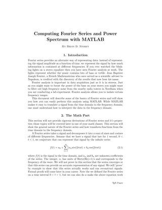
1. Computing Fourier Series and Power
Spectrum with MATLAB
By Brian D. Storey
1. Introduction
Fourier series provides an alternate way of representing data: instead of represent-
ing the signal amplitude as a function of time, we represent the signal by how much
information is contained at different frequencies. If you ever watched the blink-
ing lights on a stereo equalizer then you have seen Fourier analysis at work. The
lights represent whether the music contains lots of bass or treble. Jean Baptiste
Joseph Fourier, a French Mathematician who once served as a scientific adviser to
Napoleon, is credited with the discovery of the results that now bear his name.
Fourier analysis is important in data acquisition just as it is in stereos. Just
as you might want to boost the power of the bass on your stereo you might want
to filter out high frequency noise from the nearby radio towers in Needham when
you are conducting a lab experiment. Fourier analysis allows you to isolate certain
frequency ranges.
This document will describe some of the basics of Fourier series and will show
you how you can easily perform this analysis using MATLAB. While MATLAB
makes it easy to translate a signal from the time domain to the frequency domain,
one must understand how to interpret the data in the frequency domain.
2. The Math Part
This section will not provide rigorous derivations of Fourier series and it’s proper-
ties; those topics will be covered later in one of your math classes. This section will
show the general nature of the Fourier series and how transform functions from the
time domain to the frequency domain.
A Fourier series takes a signal and decomposes it into a sum of sines and cosines
of different frequencies. Assume that we have a signal that last for 1 second, 0 <
t < 1, we conjecture that can represent that signal by the infinite series
f(t) = a0 +
∞
n=1
(ansin(2πnt) + bncos(2πnt)) (2.1)
where f(t) is the signal in the time domain, and an and bn are unknown coefficients
of the series. The integer, n, has units of Hertz(Hz)=1/s and corresponds to the
frequency of the wave. We will not prove in this section that the series converges or
that this series can provide an accurate representation of any signal. We will ’prove’
by example to show that this series actually works and can reconstruct signals.
Formal proofs will come later in your career. Note the we defined the Fourier series
on a time interval 0 < t < 1, but we can also do a make the above equation work
TEX Paper

2. 2 Fourier Series
for any time interval. We will discuss different time intervals later, but will use
the one second interval for convenience at this point. Also note that the Fourier
representation is formally periodic, the beginning of the cycle will always equal the
end (i.e f(t = 0) = f(t = 1)).
To find the coefficients an and bn you can use the following properties. These
properties will be derived in the appendix, but we will just state the result here:
1
0
sin(2πnt)sin(2πmt)dt = 0; n and m are integers, and n = m (2.2)
1
0
sin(2πnt)sin(2πnt)dt = 1/2; n is an integer (2.3)
1
0
cos(2πnt)cos(2πmt)dt = 0; n and m are integers, and n = m (2.4)
1
0
cos(2πnt)cos(2πnt)dt = 1/2; n is an integer (2.5)
1
0
cos(2πnt)sin(2πmt)dt = 0; n and m are integers (2.6)
These properties make finding the coefficients quite easy. You can multiply both
sides of equation 2.1 by sin(2πmt) and integrate the expression over the interval
0 < t < 1. Integrating both sides of an equation is no different than multiplying
both sides by a constant: as long as you perform the same operation to both sides
of the equation the equality will hold.
1
0
f(t) = a0 +
∞
n=0
(ansin(2πnt) + bncos(2πnt)) sin(2πmt)dt. (2.7)
Applying the properties stated above, we know that the for all terms in the sum
where m does not equal n the result of the integral will be zero. We also know
that any terms that involve the product of sine and cosine will be zero. The only
remaining term in the sum will be the sine term where n = m. Therefore, equation
2.7 will reduce to
1
0
f(t)sin(2πnt)dt =
an
2
. (2.8)
Likewise, we can multiply equation 2.1 by cos(2πmt) and integrate over 0 < t < 1
to obtain the analogous result:
1
0
f(t)cos(2πnt)dt =
bn
2
. (2.9)
The coefficient a0 is even easier: we only need to integrate equation 2.1 over the
interval 0 < t < 1 to obtain.
1
0
f(t) = a0. (2.10)
Note that we have used the fact that all the sine and cosine terms integrate to zero
over the domain of interest. Now we have at our disposal equations 2.8, 2.9, & 2.10
that allow us to compute the unknown coefficients.

3. Fourier Series 3
3. Some examples
The easiest example would be to set f(t) = sin(2πt). Without even performing
the calculation (simply inspect equation 2.1) we know that the Fourier transform
should give us a1 = 1 and all other coefficients should be zero. To check that this
works, insert the test function f(t) = sin(2πt) into equations 2.8 and 2.9 to see the
result.
2
1
0
sin(2πt)sin(2πnt)dt = an. (3.1)
Using the integral properties given previously, it is clear to see that all a’s are zero
except for a1 = 1: the result we expected. All the bn coefficients are zero as well
because the integral of sin(2πt)cos(2πnt) will always be zero.
It is also easy to check that if f(t) is a constant then all the coefficients except
for a0 will be zero, providing another simple check.
Let’s try computing a Fourier series for a square wave signal that is on for half the
time interval and the off for half, i.e. f(t) = 1; 0 < t < 1/2 and f(t) = 0; 1/2 < t < 1.
To get the coefficients we apply equations 2.8 and 2.9
2
1/2
0
sin(2πnt)dt = an. (3.2)
Carrying out the integral over half the cycle (the integral over the interval 1/2 <
t < 1 will always be zero since the signal is zero during this time)
−2cos(2πnt)
2πn
1/2
0
= an (3.3)
and evaluating at t = 0 and t = 1/2 yields
1 − cos(πnt)
πn
= an. (3.4)
Therefore when n is odd,
an =
2
πn
(3.5)
and when n is even
an = 0 (3.6)
Carrying out the same operation for the coefficients bn with equation 2.9
2sin(2πnt)
2πn
1/2
0
= bn (3.7)
and evaluating at t = 0 and t = 1/2 yields
sin(πnt)
πn
= bn, (3.8)
which, for all n, is simply
bn = 0 (3.9)

4. 4 Fourier Series
0 0.1 0.2 0.3 0.4 0.5 0.6 0.7 0.8 0.9 1
−0.2
0
0.2
0.4
0.6
0.8
1
1.2
time
f(t)
n=20
n=2,000
Figure 1. Fourier reconstruction of a square wave. We see a lot of ringing in the series
until we include many points into the series.
We also need the coefficient, a0, which is obtained by integrating equation 2.1 over
the time interval
a0 =
1/2
0
dt = 1/2. (3.10)
Now we can plot the Fourier series representation using MATLAB and see how
the series does at reproducing the original signal. If we plot the first 20 terms in the
sum, we see the general shape of the original function but we see a lot of ’ringing’. As
we plot more terms, we see the original function is represented quite accurately. In
general Fourier series can reconstruct a signal with a small number of modes if the
original signal is smooth. Discontinuities require many high frequency components
to construct the signal accurately.
For reference, the MATLAB code that generated this figure is given below:
N = 2000;
x = [0:100]/100;
f = ones(1,101)*1/2;
for i = 1:2:N
a = 2/pi/i;
f = f+ a*sin(2*pi*i*x);
end
plot(x,f)
4. Fourier Transform of Discrete Data
When we are working with data that we have acquired with the DAQ card we have
discrete data points, not an analytical function that we can analytically integrate.
It turns out that taking a Fourier transform of discrete data is done by simply
taking a discrete approximation to the integrals (2.8, 2.9, 2.10).

5. Fourier Series 5
0 0.1 0.2 0.3 0.4 0.5 0.6 0.7 0.8 0.9 1
−1
−0.8
−0.6
−0.4
−0.2
0
0.2
0.4
0.6
0.8
1
time
f(t)
t
1
t
2
t
3
t
4
t
5
t
6
t
7
t
8
A
1
A
2
A
3
A4
A
5
A
6
A7
Figure 2. Schematic of trapezoidal rule applied to the function f(t) = sin(2πt) sampled
at 8 points. The trapezoidal rule simply computes the area of each block and sums them
up.
The discrete integral can be computed using the trapezoidal rule. The trape-
zoidal rule simply breaks up a function into several trapezoids and sums the area,
see Figure 2
In Figure 2 we see that there are seven blocks (Aj) and 8 data points (tj). To
compute the area, Aj, of the jth
trapezoidal block we use
Aj =
f(tj) + f(tj+1)
2
(tj+1 − tj) (4.1)
For now, let’s assume that the points tj are equally spaced such that tj+1 −tj =
∆t. Therefore the total area is
A = ∆t
f(t1) + f(t2)
2
+
f(t2) + f(t3)
2
+ ...
f(t6) + f(t6)
2
+
f(t7) + f(t8)
2
,
(4.2)
which generalizes to
f(t)dt = ∆t

f(t1)/2 + f(tn)/2 +
N−1
j=2
f(tj)

 (4.3)
The trapezoidal rule provides a general mechanism for approximating integrals.
To compute the Fourier coefficient, an, you simply need to apply the trapezoid
rule to the function multiplied by the function sin(2πnt), specifically,
an = ∆t[sin(2πnt1)f(t1) + sin(2πntN )f(tN ) + 2
N−1
j=2
sin(2πntj)f(tj)] (4.4)
Exercise FS 1: Write a general MATLAB function that takes a two
vectors, x and y as input, assumes y is a function of x and computes

6. 6 Fourier Series
the integral
x(N)
x(1)
y(x)dx using the trapezoidal rule (equation 4.3). Some
MATLAB functions that may be useful, though surely not necessary, are
length, sum, y(end), diff, and unique. Equation 4.3 assumes that the
points in x are equally spaced - your function can make this assumption
as well. Test the numerical integral on the functions sin(2πx) and x2
on the interval of 0 < x < 1. Does the numerical approximation match
the analytical result? After you write your function, which you can
name integral, you should be able to go to the MATLAB prompt and
issue the following commands: x = [0:100]/100; y = sin(2*pi*x);
to define x and y. You should then be able to type integral(y,x) with
no semi-colon to get the value of the integral returned at the prompt.
Advanced questions Derive the expression for the numerical integral
where the points in x are not equally spaced. Adapt your function to
work for a general spacing in x. Test your function using an x defined by
the logspace command. The error of the approximation is defined as
the difference between the ’true’ analytical integral and the numerical
integral. Compute the error in the integral for sin(2πx) in a range of 10
to 10,000 data points. Plot on a log-log plot the error vs. the number of
data points.
Exercise FS 2: Write a general MATLAB function that takes a discrete
function f(tj) and a frequency n as input and computes the discrete
Fourier coefficient using equation 4.4. Assume that the input function
spans from 0 < t < 1 and that the data points are equally spaced in
time on that 0 < t < 1 interval: i.e. ∆t = 1/(N − 1) where ∆t is the
spacing in time between points and N is the number of points used to
represent the function f. Create a discrete function using 20 points that
corresponds to the square wave that we used in Figure 1. For example: f
= [ones(1,10) zeros(1,10)]; defines the square wave. Numerically
compute a few different Fourier coefficients (both an and bn coefficients)
with your MATLAB function: try n=0,1,2,3 and 4. Show that the nu-
merical result is in good agreement with the analytical expression for
the square wave, equation 3.5.
Advanced questions Write your function to compute the Fourier co-
efficients for all frequencies, n. You can only compute up to (N − 1)/2
Fourier coefficients where N is the number of points used to describe
your function. Vary the number of discrete points and comment on the
accuracy of the discrete approximation. The error is defined as the dif-
ference between the numerical result and the analytical. Read the help
on the wavplay and wavrecord commands. Record 1 second of sound
(try whistling at a constant pitch) through your computers microphone.
Find the Fourier coefficients using your MATLAB function: plot the
Fourier coefficients vs. frequency.
5. The FFT
Despite the fact that we presented the discrete transform, we will not use it. There
is better way to compute the Fourier transform of discrete data called the Fast

7. Fourier Series 7
Fourier Transform (FFT). The FFT was a truly revolutionary algorithm that made
Fourier analysis mainstream and made processing of digital signals commonplace.
The power of the FFT is that it allows you to compute the Fourier coefficients,
hold on to your hats, fast. Let’s count how many operations the computer must
do to perform the Discrete Fourier transform using the trapezoidal rule. For each
mode, we would need to make N multiplications and N additions (see equation
4.4). We would need to perform this operation for all N Fourier modes. The result
is that the total computational cost scales as N2
; i.e. you double the number of data
points and you quadruple the number of operations. For a data set of 1,000 points
the computer would need to do approximately 1,000,000 operations to compute the
transform in this manner. The signals we want to take a Fourier transform of are
often quite long. To sample music at a rate that sounds pleasing, we would like a
40,000 Hz as a sample rate. A few seconds of sound quickly becomes a lot of data.
The FFT algorithm plays a few tricks and can take a Fourier transform of a
discrete set of data in NLog2(N) operations. For 1 second of data sampled at 40,000
Hz this translates into a computation that can be reduced by a factor of 2000, an
enormous savings! One thing to keep in mind is that the cost savings of the FFT only
applied when the number of points is a power of 2 (i.e. N = 2, 4, 8, 16, 32, 64, 128, ..).
The FFT has become such a commonplace algorithm that it is built into MAT-
LAB. To take a Fourier transform of data you simply type fft(data);. This is
the point where old people will tell you ’back in my day we wrote our own FFT
solvers and liked it’. Don’t believe them. An efficient FFT is quite complex and
nobody has ever enjoyed writing their own. Appreciate the power of fft(data).
MATLAB makes taking an FFT easy: the only hard part comes in deciphering
what the algorithm has given you back.
(a) Deciphering the FFT Data
There are two things that are different about the FFT implementation in MAT-
LAB than the presentation that we gave in the first section: the FFT uses complex
numbers (i =
√
−1) and the FFT computes positive and negative frequencies. There
is also some differences in scaling factors that we will explain. Many of the reasons
the MATLAB algorithm works the way it does is for generality (it works for all
data), convention, and algorithmic efficiency.
At this point many of you may have some or no experience with complex num-
bers. Use of complex numbers introduces some mathematical simplicity in Fourier
transform algorithms and provides a convenient representation. The purpose of this
section is to allow to interpret the results, which means we need to explain a little
bit about complex numbers.
The imaginary number i (sometimes j is used) is defined as the
√
−1. A complex
number, c, is typically written
c = a + bi (5.1)
where a is called the real part and b is called the imaginary part: in this equation
a and b are real (ordinary) numbers. The product of a complex number is given as
cc = (a + bi)(a + bi) = a2
− b2
+ 2abi. (5.2)
The complex conjugate of c is denoted and defined as
¯c = (a − bi). (5.3)

8. 8 Fourier Series
−1 −0.8 −0.6 −0.4 −0.2 0 0.2 0.4 0.6 0.8 1
−1
−0.8
−0.6
−0.4
−0.2
0
0.2
0.4
0.6
0.8
1
0.3 + 0.5 i
−0.1 − 0.8 i
real
imaginary
Figure 3. Representation of complex numbers on the two dimensional complex plane. It
is easy to see that the definition of the absolute value of a complex number is simply the
distance of the number from the origin.
The absolute value of c is given as
|c| =
√
c¯c = a2 + b2 (5.4)
Note that in the above expression we made use of the fact that i2
= −1. Real
numbers are often represented on the real number line and complex numbers are
often visualized on the two dimensional complex plane, see Figure 3. In the complex
plane it is clear to see that the absolute value is simply the distance of the complex
number from the origin.
OK, back to the FFT algorithm. Let’s type an example to demonstrate the
FFT. Go to your MATLAB prompt and type in a time vector >>t = [0:7]’/8.
This will create a list of numbers from 0 to 0.875 in increments of 1/8. When using
the FFT the last data point which is the same as the first (since the sines and
cosines are periodic) is not included. Note that the time vector does not go from
0 to 1. We will later show what happens if your time vector goes from 0 to 1.
Create a list of numbers f which corresponds to sin(2πt). At the prompt type >>f
= sin(2*pi*t);. Now take the FFT by typing fft(f) (note that you can leave off
the semi-colon so MATLAB will print). MATLAB should return
0.0000
-0.0000 - 4.0000i
0.0000 - 0.0000i
0.0000 - 0.0000i
0.0000
0.0000 + 0.0000i
0.0000 + 0.0000i
-0.0000 + 4.0000i
The ordering of the frequencies is as follows [0 1 2 3 4 -3 -2 -1]. Note that
8 discrete data points yields 8 Fourier coefficients and the highest frequency that will

9. Fourier Series 9
be resolved is N/2. The order that the coefficients come in is often called reverse-
wrap-around order. The first half of the list of numbers is the positive frequencies
and the second half is the negative frequencies. The real part of the FFT corresponds
to the cosines series and the imaginary part corresponds to the sine. When taking
an FFT of a real number data set (i.e. no complex numbers in the original data) the
positive and negative frequencies turn out to be complex conjugates (the coefficient
for frequency = 1 is the complex conjugate of frequency=-1). Also, the MATLAB
FFT returns data that needs to be divided by N/2 to get the coefficients that we
used in the sin and cos series. To obtain the coefficients an and bn we use the
following formulas, where cn is the coefficient of the MATLAB FFT.
an = −
1
2N
imag(cn), 0 < n <
N
2
(5.5)
bn =
1
2N
real(cn), 0 < n <
N
2
. (5.6)
The notation imag(c) means you take the imaginary part of cn. The above expres-
sions are appropriate for 0 < n < N/2. Applying these expressions to the above
example shows the result is a1 = 1: which is the answer that we expect. The values
of the FFT in the frequencies negative frequencies provide no new information since
the coefficients are simply complex conjugates.
Let’s try another example. Create a list of numbers f which corresponds to
cos(4πt). At the prompt type >>f = cos(4*pi*t);. Now take the FFT by typing
fft(f) (note that you can leave off the semi-colon). MATLAB should return
-0.0000
-0.0000 + 0.0000i
4.0000 - 0.0000i
0.0000 + 0.0000i
0.0000
0.0000 - 0.0000i
4.0000 + 0.0000i
-0.0000 - 0.0000i
Applying the transformation equations 5.5 and 5.6 to get coefficients of the sine
and cosine series results in b2 = 1: the result that we expect.
Now try the following commands
>> t = [0:7]’/8;
>> f = sin(2*pi*t);
>> f = fft(f);
>> f(1)
The value of f(1) should be very small, but not zero. Typically it will have a value
of approximately 10−15
. The value should be zero, but what you are witnessing is
numerical roundoff error. Floating point numbers cannot be represented exactly on
the computer and therefore you will often find numbers that should be zero are
small, but never exactly 0.
As a final example let’s show what happens if you define the discrete data to
run from 0 < t < 1. try typing the following commands;
>> t = [0:7]’/7;
>> f = sin(2*pi*t);

10. 10 Fourier Series
>> f = fft(f)
The result should appear as
-0.00000000000000
1.36929808581104 - 3.30577800969654i
-0.62698016883135 + 0.62698016883135i
-0.50153060757593 + 0.20774077960317i
-0.48157461880753
-0.50153060757593 - 0.20774077960317i
-0.62698016883135 - 0.62698016883135i
1.36929808581104 + 3.30577800969654i
We see that the result is not what you would want. If you increase the number of
points the closer the result will look to what you would like. Try the same example
as above but use 16 data points, then try 64. As you increase the number of points
the smaller the spurious data becomes. In any case, the way the discrete FFT is
defined, the last point of a periodic function is not included.
You can also take the inverse Fourier transform to move data from the frequency
domain to the time domain. The inverse FFT command is given as ifft. Try taking
the Fourier transform of a function, then apply the inverse to see that you get the
proper result back.
6. Power Spectrum
In the previous section we saw how to unwrap the FFT and get back the sine and
cosine coefficients. Usually we only care how much information is contained at a
particular frequency and we don’t really care whether it is part of the sine or cosine
series. Therefore, we are interested in the absolute value of the FFT coefficients.
The absolute value will provide you with the total amount of information contained
at a given frequency, the square of the absolute value is considered the power of
the signal. Remember that the absolute value of the Fourier coefficients are the
distance of the complex number from the origin. To get the power in the signal at
each frequency (commonly called the power spectrum) you can try the following
commands.
>> N = 8; %% number of points
>> t = [0:N-1]’/N; %% define time
>> f = sin(2*pi*t); %%define function
>> p = abs(fft(f))/(N/2); %% absolute value of the fft
>> p = p(1:N/2).^2 %% take the positve frequency half, only
This set of commands will return something much easier to understand, you should
get 1 at a frequency of 1 and zeros everywhere else. Try substituting cos for sin
in the above commands, you should get the same result. Now try making >>f =
sin(2*pi*t) + cos(2*pi*t). This change should result in twice the power con-
tained at a frequency of 1.
Thus far we have looked at data that is defined on the time interval of 1 second,
therefore we could interpret the location in the number list as the frequency. If the
data is taken over an arbitrary time interval we need to map the index into the
Fourier series back to a frequency in Hertz. The following m-file script will create
something that might look like data that we would obtain from a sensor. We will

11. Fourier Series 11
0 2 4 6 8 10 12 14 16 18 20
10
−15
10
−10
10
−5
10
0
frequency (Hz)
power
Figure 4. Power spectrum of a 10 Hz sine wave sampled at 10,000 points over 3.4
seconds. As expected we get a very strong peak at a frequency of 10 Hz.
’sample’ 10,000 points over an interval of 3.4 seconds. The signal will be a 10 Hz
sine wave. We will compute the power and plot power vs. frequency in Hertz.
N = 10000; %% number of points
T = 3.4; %% define time of interval, 3.4 seconds
t = [0:N-1]/N; %% define time
t = t*T; %% define time in seconds
f = sin(2*pi*10*t); %%define function, 10 Hz sine wave
p = abs(fft(f))/(N/2); %% absolute value of the fft
p = p(1:N/2).^2 %% take the power of positve freq. half
freq = [0:N/2-1]/T; %% find the corresponding frequency in Hz
semilogy(freq,p); %% plot on semilog scale
axis([0 20 0 1]); %% zoom in
The result of these commands is shown in Figure 4
Exercise FS 3: Create a MATLAB function that takes a data set and
returns the power spectrum. The input arguments to the function should
be the data and the actual time spanned by the data. The function
should return two vectors, the frequency and the power. Note that we
already did most of this for you in the last set of MATLAB code.
Exercise FS 4: The MATLAB command wavrecord can be used to
acquire data from your computers microphone (check the help). The
following commands will record and then play back 5 seconds of data
sampled at 44,100 Hz (a standard audio rate) from your computers
microphone and speaker.
Fs = 44100;
y = wavrecord(5*Fs, Fs);
wavplay(y, Fs);

12. 12 Fourier Series
0 5 10 15 20 25 30
0
0.1
0.2
0.3
0.4
0.5
0.6
0.7
0.8
0.9
1
frequency (Hz)
power
Figure 5. Power spectrum of a 10 Hz sine wave sampled at 10,000 points over 3.4 seconds
with random noise of amplitude 4 superimposed. The FFT can still extract a very strong
signal at a frequency of 10 Hz despite the fact that we can’t see the original signal in the
time domain.
Now you can plot this recorded data (plot(y)) to see your voice plotted
in the time domain. Take the power spectrum of the data and see the
frequency content of your voice. Try whistling at a constant pitch and
record again. Plot the power spectrum and see if you can get a spike at
a single frequency.
7. Fourier transform as a filter
The Fourier transform is useful for extracting a signal from a noisy background. As
an example, lets modify the last program that you wrote. After you define f and
before taking the fft add the line
f = f + 4*randn(1,N);
This command will add a random number that will overwhelm the signal. To see
the noise, plot the signal, i.e add the command plot(f), and you will see little
evidence of the original signal. If we plot the power spectrum of the signal we find
out that the 10 Hz signal stands out from the noisy background as shown in Figure
5.
This example demonstrates one of the useful features of the Fourier transform.
When you take actual data using the data card and perform a power spectrum
you will often find that there is a fairly strong signal at 60 Hz. This corresponds
to the AC frequency of the power that is being delivered to the wall sockets. The
wires on your laboratory set-up will act like antennae picking up 60 Hz noise. The
FFT would allow you to remove this spurious noise. Also, the FFT can be used to
extract signals buried in a noisy background.
A simple way to filter the noise out of Figure 5 would be to apply a simple
threshold filter. After taking the power spectrum, you could isolate the peak by
searching for the frequencies that contain most of the energy. You could then set

13. Fourier Series 13
the coefficients of FFT at frequencies that have little power to zero. The result
would be the primary signal with no noise.
You could also build the equivalent to a stereo equalizer using the Fourier trans-
form. You can transform your signal to frequency domain and simply amplify (or
attenuate) coefficients in certain regions of frequency domain (i.e. boost the bass
and dampen the treble). You could then FFT the signal back to the time domain
and play it.
Exercise FS 5 Noisy electrical components. Write a program using
MATLAB’s Data Acquisition Toolbox that will sample data from one
channel for a few seconds. Take the signal from the function generator
and run the wires to the proto-board. Now run the wires from the proto-
board to the terminal block so that your DAQ card can measure the
signal (Note at this point your could have sent the signal straight to the
terminal block). Start the function generator at a known amplitude and
frequency. Acquire data and take the power spectrum, the result should
be dominated by the frequency you set on the function generator. Look
at the power spectrum and look for evidence of 60 Hz noise. Increase
the length of the wire and see if the power contained at 60 Hz changes.
Are there any other dominant frequencies? What is the level of the
background noise? Run the signal through a resistor placed on the proto-
board. Does the power in the noise (relative to the signal) change? Try
running the signal through a few resistors.
Appendix A.
In the first section we presented several integral results that we used to derive
properties of the Fourier transform. Let us show how these were obtained. Let’s
start with
1
0
sin(2πnt)sin(2πmt)dt (A 1)
If you remember your trig identities (don’t worry, I forget them so I always look
them up or re-derive them every time!) you might remember that
cos(a + b) = cos(a)cos(b) − sin(a)sin(b) (A 2)
and
cos(a − b) = cos(a)cos(b) + sin(a)sin(b) (A 3)
Therefore we can write
2sin(a)sin(b) = cos(a − b) − cos(a + b). (A 4)
Using this expression we write the integral as
1
2
1
0
(cos(2πnt − 2πmt) − cos(2πnt + 2πmt)) dt (A 5)
which reduces to
1
2
1
0
(cos(2πt(n − m)) − cos(2πt(n + m))) dt. (A 6)

14. 14 Fourier Series
Performing the integral yields
1
2
sin(2πt(n − m))
2π(n − m)
−
sin(2πt(n + m))
2π(n + m)
1
0
. (A 7)
Evaluating at zero and one gives you
sin(2π(n − m))
4π(n − m)
−
sin(2π(n + m))
4π(n + m)
(A 8)
Evaluating this expression where m and n are integers and they are not equal yields
0. For the case where n=m, we need to return to equation A 5. Substituting n=m
we obtain,
1
2
1
0
(1 − cos(2πnt + 2πnt)) dt (A 9)
Performing the integral is
1
2
−
sin(4πtn)
4πn
1
0
=
1
2
. (A 10)
These results were the ones that were presented in main text.
To obtain the result for the integral
1
0
cos(2πnt)cos(2πmt)dt (A 11)
we proceed in the same manner, only we use the identity
2cos(a)cos(b) = cos(a − b) + cos(a + b). (A 12)
By inspection you can see this expression will reduce to those obtain previously.
Finally we will compute the integral
1
0
sin(2πnt)cos(2πmt)dt. (A 13)
For this expression we use the trig identity
2cos(a)sin(b) = sin(a + b) − sin(a − b). (A 14)
Using this expression we write the integral as
1
2
1
0
(sin(2πt(n + m)) − sin(2πt(n − m))) dt. (A 15)
Performing the integral is
1
2
cos(2πt(n + m))
2π(n + m)
−
cos(2πt(n − m))
2π(n − m)
1
0
. (A 16)
Evaluating at zero and one gives you
cos(2π(n − m)) − 1
4π(n − m)
−
cos(2π(n + m)) − 1
4π(n + m)
(A 17)

15. Fourier Series 15
Evaluating this expression where m and n are integers and they are not equal yields
0. For the case where n=m, we need to return to equation A 15. Substituting n=m
we obtain,
1
2
1
0
sin(4πnt)dt = 0. (A 18)
We have therefore provided a proof for all the integral identities used in the deriva-
tion of the Fourier series.