This document provides a linear algebra review that covers topics such as vectors, matrices, eigenvalues, eigenvectors, linear independence, and the singular value decomposition. It defines key terms such as the dot product, transpose, inverse, determinant, rank, and orthogonality. Examples are provided to illustrate matrix operations and properties. The singular value decomposition is introduced as a way to write any matrix as the product of three matrices involving orthogonal matrices and a diagonal matrix of singular values.

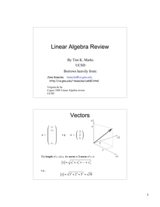
1. Linear Algebra Review
By Tim K. Marks
UCSD
Borrows heavily from:
Jana Kosecka kosecka@cs.gmu.edu
http://cs.gmu.edu/~kosecka/cs682.html
Virginia de Sa
Cogsci 108F Linear Algebra review
UCSD
Vectors
The length of x, a.k.a. the norm or 2-norm of x, is
x = x12 + x 2 + L + x n
2 2
e.g.,
x = 32 + 2 2 + 5 2 = 38
!
!
1

2. Good Review Materials
http://www.imageprocessingbook.com/DIP2E/dip2e_downloads/review_material_downloads.htm
(Gonzales & Woods review materials)
Chapt. 1: Linear Algebra Review
Chapt. 2: Probability, Random Variables, Random Vectors
Online vector addition demo:
http://www.pa.uky.edu/~phy211/VecArith/index.html
2

3. Vector Addition
u+v
v
u
Vector Subtraction
u-v
u
v
3

4. Example (on board)
Inner product (dot product) of
two vectors
#6& "4%
% ( $ '
a =%2 ( b = $1'
%"3(
$ ' $5'
# &
a " b = aT b
! ! #4&
% (
= [6 2 "3] %1(
! %5(
$ '
= 6 " 4 + 2 "1+ (#3) " 5
= 11
!
!
!
4

5. Inner (dot) Product
The inner product is a SCALAR.
v α
u
5

6. Transpose of a Matrix
Transpose:
Examples:
If , we say A is symmetric.
symmetric.
Example of symmetric matrix
6

7. 7

8. 8

9. 9

10. Matrix Product
Product:
A and B must have
compatible dimensions
In Matlab: >> A*B
Examples:
Matrix Multiplication is not commutative:
10

11. Matrix Sum
Sum:
A and B must have the
same dimensions
Example:
Determinant of a Matrix
Determinant: A must be square
Example:
11

12. Determinant in Matlab
Inverse of a Matrix
If A is a square matrix, the inverse of A, called A-1,
satisfies
AA-1 = I and A-1A = I,
Where I, the identity matrix, is a diagonal matrix
with all 1’s on the diagonal.
"1 0 0%
"1 0% $ '
I2 = $ ' I3 = $0 1 0'
#0 1&
$0 0 1'
# &
!
!
12

13. Inverse of a 2D Matrix
Example:
Inverses in Matlab
13

14. Other Terms
14

15. Matrix Transformation: Scale
A square diagonal matrix scales each dimension by
the corresponding diagonal element.
Example:
"2 0 0% "6% "12%
$ ' $ ' $ '
$0 .5 0' $8' = $ 4 '
$
#0 0 3'& $ '
#10& $ '
#30&
!
15

16. http://www.math.ubc.ca/~cass/courses/m309-8a/java/m309gfx/eigen.html
16

17. Some Properties of
Eigenvalues and Eigenvectors
– If λ1, …, λn are distinct eigenvalues of a matrix, then
the corresponding eigenvectors e1, …, en are linearly
independent.
– A real, symmetric square matrix has real eigenvalues,
with eigenvectors that can be chosen to be orthonormal.
Linear Independence
• A set of vectors is linearly dependent if one of
the vectors can be expressed as a linear
combination of the other vectors.
Example: "1% "0% "2%
$' $' $'
$0' , $1' , $1'
$' $' $'
#0& #0& #0&
• A set of vectors is linearly independent if none
of the vectors can be expressed as a linear
!
combination of the other vectors.
Example: "1% "0% "2%
$' $' $'
$0' , $1' , $1'
$' $' $'
#0& #0& #3&
!
17

18. Rank of a matrix
• The rank of a matrix is the number of linearly
independent columns of the matrix.
Examples: "1 0 2%
$
0 1 1
' has rank 2
$ '
$0 0 0'
# &
"1 0 2%
$ '
! $0 1 0' has rank 3
$0 0 1'
# &
• Note: the rank of a matrix is also the number of
linearly!independent rows of the matrix.
Singular Matrix
All of the following conditions are equivalent. We
say a square (n × n) matrix is singular if any one
of these conditions (and hence all of them) is
satisfied.
– The columns are linearly dependent
– The rows are linearly dependent
– The determinant = 0
– The matrix is not invertible
– The matrix is not full rank (i.e., rank < n)
18

19. Linear Spaces
A linear space is the set of all vectors that can be
expressed as a linear combination of a set of basis
vectors. We say this space is the span of the basis
vectors.
– Example: R3, 3-dimensional Euclidean space, is
spanned by each of the following two bases:
"1% "0% "0% "1% "0% "0%
$' $' $' $' $' $'
$0' , $1' , $0' $0' , $1' , $0'
$' $' $'
#0& #0& #1& $' $' $'
#0& #2& #1&
! !
Linear Subspaces
A linear subspace is the space spanned by a subset
of the vectors in a linear space.
– The space spanned by the following vectors is a
two-dimensional subspace of R3.
"1% "0%
$' $'
What does it look like?
$0' , $1'
$0' $0'
#& #&
– The space spanned by the following vectors is a
two-dimensional subspace of R3.
! "1% "0%
$' $' What does it look like?
$1' , $0'
$' $'
#0& #1&
!
19

20. Orthogonal and Orthonormal
Bases
n linearly independent real vectors
span Rn, n-dimensional Euclidean space
• They form a basis for the space.
– An orthogonal basis, a1, …, an satisfies
ai ⋅ aj = 0 if i j
– An orthonormal basis, a1, …, an satisfies
ai ⋅ aj = 0 if i j
ai ⋅ aj = 1 if i = j
– Examples.
Orthonormal Matrices
A square matrix is orthonormal (also called
unitary) if its columns are orthonormal vectors.
– A matrix A is orthonormal iff AAT = I.
• If A is orthonormal, A-1 = AT
AAT = ATA = I.
– A rotation matrix is an orthonormal matrix with
determinant = 1.
• It is also possible for an orthonormal matrix to have
determinant = -1. This is a rotation plus a flip (reflection).
20

21. SVD: Singular Value Decomposition
Any matrix A (m × n) can be written as the product of three
matrices:
A = UDV T
where
– U is an m × m orthonormal matrix
– D is an m × n diagonal matrix. Its diagonal elements, σ1, σ2, …, are
called the singular values of A, and satisfy σ1 ≥ σ2 ≥ … ≥ 0.
– V is an n × n orthonormal matrix
Example: if m > n
A U D VT
"• • •% "( ( ( (% "*1 0 0 %
$ ' $ ' $ '"
$• • •' $ | | | |' $ 0 * 2 0 '$+ v1
T
,%
'
$• • •' = $u1 u2 u3 L um ' $ 0 0 * n '$ M M M'
$ ' $ ' $ '$
$• • •' $ | | | |' $ 0 0 0 '#+ v n
T
,'
&
$
#• ' $
• •& #) ) ) )& ' $
#0 0 0 ' &
!
SVD in Matlab
>> x = [1 2 3; 2 7 4; -3 0 6; 2 4 9; 5 -8 0]
x=
1 2 3
2 7 4
-3 0 6
2 4 9
5 -8 0
>> [u,s,v] = svd(x)
u= s=
-0.24538 0.11781 -0.11291 -0.47421 -0.82963 14.412 0 0
-0.53253 -0.11684 -0.52806 -0.45036 0.4702 0 8.8258 0
-0.30668 0.24939 0.79767 -0.38766 0.23915 0 0 5.6928
-0.64223 0.44212 -0.057905 0.61667 -0.091874
0 0 0
0.38691 0.84546 -0.26226 -0.20428 0.15809
0 0 0
v=
0.01802 0.48126 -0.87639
-0.68573 -0.63195 -0.36112
-0.72763 0.60748 0.31863
21

22. Some Properties of SVD
– The rank of matrix A is equal to the number of nonzero
singular values σi
– A square (n × n) matrix A is singular iff at least one of
its singular values σ1, …, σn is zero.
Geometric Interpretation of SVD
If A is a square (n × n) matrix,
A U D VT
"• • •% " ( L ( % "*1 0 0 %"+ v1 T
,%
$ ' $ ' $ '$ '
$• • •' = $u1 L un ' $ 0 * 2 0 '$ M M M'
$• • •'
# & $ ) L ) ' $ 0 0 * n '$+ v T
# & # &# n ,'
&
– U is a unitary matrix: rotation (possibly plus flip)
– D is a scale matrix
T
! – V (and thus V ) is a unitary matrix
Punchline: An arbitrary n-D linear transformation is
equivalent to a rotation (plus perhaps a flip), followed by a
scale transformation, followed by a rotation
Advanced: y = Ax = UDV Tx
T
– V expresses x in terms of the basis V.
– D rescales each coordinate (each dimension)
– The new coordinates are the coordinates of y in terms of the basis U
22