SlideShare ist ein Scribd-Unternehmen logo
1 von 43
Introduction:
• Generally, the WKB approximation or WKB
method is a method for finding approximate
solutions to linear differential equations with
spatially varying coefficients.
• In Quantum Mechanics it is used to obtain
approximate solutions to the time-
independent Schrodinger equation in one
dimension.
Applications in Quantum Mechanics
In quantum mechanics it is useful in
1. Calculating bound state energies (Whenever
the particle cannot move to infinity)
2. Transmission probability through potential
barriers.
These are given in next slides.
Main idea:
• If potential 𝑽(𝒙) is constant and energy 𝐸 of the particle is 𝑬 > 𝑽,
then the particle wave function has the form
𝜓 𝑥 = 𝐴𝑒±𝑖𝑘𝑥 where 𝑘 = √(2𝑚(𝐸−𝑉))
ℏ
(+) sign indicates : particle travelling to right
(-) sign indicates : particle travelling to left
• General solution : Linear superposition of the two.
• The wave function is oscillatory, with fixed wavelength, 𝜆 =
2𝜋
𝑘
.
• The amplitude (A) is fixed.
• If V (x) is not constant, but varies slow in comparison
with the wavelength λ in a way that it is essentially
constant over many λ, then the wave function is
practically sinusoidal, but wavelength and amplitude
slowly change with x. This is the inspiration behind
WKB approximation. In effect, it identifies two
different levels of x-dependence :- rapid oscillations,
modulated by gradual variation in amplitude and
wavelength.
• If E<V and V is constant, then wave function is
𝜓 𝑥 = 𝐴𝑒±𝜅𝑥
where κ = √(2𝑚(𝑉−𝐸))
ℏ
If 𝑽(𝒙) is not constant, but varies slowly in
comparison with 1
𝜅 , the solution remain
practically exponential, except that 𝐴 and 𝜅 are
now slowly-varying function of 𝑥.
Failure of this idea
There is one place where this whole program is
bound to fail, and that is in the immediate vicinity
of a classical turning point, where 𝐸 ≈ 𝑉. For here
𝜆(𝑜𝑟 1
𝜅)) goes to infinity and 𝑉(𝑥) can hardly be
said to vary “slowly” in comparison. A proper
handling of the turning points is the most difficult
aspect of the WKB approximation, though the final
results are simple to state and easy to implement.
The diagram showing turning points is given in next
slide.
The WKB approximation
V(x)
E
Turning points
The Classical Region
• Let's now solve the Schrödinger equation using WKB
approximation
−ℏ2
2𝑚
𝑑2 𝜓
𝑑𝑥2 + 𝑉 𝑥 𝜓 = 𝐸𝜓 can be rewritten in the
following way:
𝑑2 𝜓
𝑑𝑥2 = −
𝑝2
ℏ2 𝜓 ; 𝑝 𝑥 = 2𝑚(𝐸 − 𝑉(𝑥)) is the
classical formula for the momentum of a particle with
total energy 𝐸 and potential energy 𝑉(𝑥). Let’s
assume 𝐸 > 𝑉(𝑥), so that 𝑝(𝑥) is real. This is the
classical region , as classically the particle is confined
to this range of 𝑥. The classical and non-classical region
is shown in the diagram on the next slide.
The WKB approximation
V(x)
E
Classical region (E>V)
Non-classical
region (E<V)
Fig: Classically, the particle is confined to the region where 𝑬 ≥ 𝑽(𝒙)
The function 𝜓
In general, 𝜓 is some complex function; we can
express it in terms of its amplitude 𝐴(𝑥), and its
phase, 𝜙(𝑥) – both of which are real :
𝜓 𝑥 = 𝐴(𝑥)𝑒 𝑖𝜙(𝑥)
Solving the Schrödinger equation
𝜓 𝑥 = 𝐴(𝑥)𝑒 𝑖𝜙(𝑥)
Using prime to denote the derivative with respect to
𝑥, we find:
𝑑𝜓
𝑑𝑥
= (𝐴′+𝑖𝐴𝜙′)𝑒 𝑖𝜙
and
𝑑2 𝜓
𝑑𝑥2
= [𝐴′′
+2𝑖𝐴′
𝜙′
+ 𝑖𝐴𝜙′′
− 𝐴 𝜙′ 2
]𝑒 𝑖𝜙
Putting all these into
𝑑2 𝜓
𝑑𝑥2 = −
𝑝2
ℏ2 𝜓 (From Schrödinger
equation ) , we get
𝐴′′
+ 2𝑖𝐴′
𝜙′
+ 𝑖𝐴𝜙′′
− 𝐴 𝜙′ 2
= −
𝑝2
ℏ2
𝐴
Solving for real and imaginary parts we get,
𝐴′′ − 𝐴 𝜙′ 2 = −
𝑝2
ℏ2
𝐴
𝐴′′ = 𝐴 (∅′)2−
𝑝2
ℏ2
𝐴′′
𝐴
= (∅′)2−
𝑝2
ℏ2
The above equation cannot be solved in general, so we use WKB
approximation: we assume amplitude A varies slowly, so that the
A’’ term is negligible. We assume that 𝐴′′
𝐴 << [(∅′)2−
𝑝2
ℏ2].
Therefore, we drop that part and we get
𝜙 𝑥 = ±
1
ℏ
𝑝 𝑥 𝑑𝑥
And from second equation, we get
2𝐴′
𝜙′
+ 𝐴𝜙′′
= 0
𝐴2
𝜙′ ′
= 0
𝐴 =
𝐶
𝜙′
Where C is real constant.
Thus from the previous slides from the equations
and making ‘C’ a complex constant, we get
𝜓(𝑥) ≅
𝐶
𝑝(𝑥)
𝑒±
𝑖
ℏ
𝑝 𝑥 𝑑𝑥
And the general solution can be written as
𝜓(𝑥) ≅
1
𝑝(𝑥)
𝐶1 𝑒
𝑖
ℏ
𝑝 𝑥 𝑑𝑥
+ 𝐶2 𝑒
−𝑖
ℏ
𝑝 𝑥 𝑑𝑥
where 𝐶1 and 𝐶2 are constants.
Alternate approach
In this approach, the wave function is expanded
in powers of ℏ .
Let, the wave function be:
𝜓 = 𝐴𝑒
𝑖
ℏ
𝑆(𝑥)
Using this in:
𝑑2 𝜓
𝑑𝑥2 + 𝑘2
𝜓 = 0, we get
𝑑𝑆
𝑑𝑥
2
− 𝑖ℏ
𝑑2 𝑆
𝑑𝑥2 − 𝑘2
ℏ2
= 0 --------(1)
Expanding S(x) in powers of ℏ2
:
𝑆 𝑥 = 𝑆0 𝑥 + 𝑆1 𝑥 ℏ + 𝑆2 𝑥
ℏ2
2
+ ⋯
∴ 1 ⟹
𝑑𝑆0
𝑑𝑥
2
− 𝑘2
ℏ 2
+ 2
𝑑𝑆0
𝑑𝑥
𝑑𝑆1
𝑑𝑥
− 𝑖
𝑑2 𝑆0
𝑑𝑥2 ℏ = 0 ;
(neglecting higher powers of ℏ).
where 𝑘2
ℏ 2
= 2𝑚[𝐸 − 𝑉(𝑥)]
For the above equation to be valid, the coefficient
of each power of ℏ must vanish separately,
𝑑𝑆0
𝑑𝑥
2
− 𝑘2
ℏ 2
= 0 𝑜𝑟
𝑑𝑆0
𝑑𝑥
= ±𝑘ℏ
⟹ 𝑆0 x = ± 𝑘ℏ𝑑𝑥
and, 2
𝑑𝑆0
𝑑𝑥
𝑑𝑆1
𝑑𝑥
− 𝑖
𝑑2 𝑆0
𝑑𝑥2 = 0
𝑜𝑟,
𝑑𝑆1
𝑑𝑥
=
𝑖
2𝑘
𝑑𝑘
𝑑𝑥
; using the value of 𝑆0(x)
𝑜𝑟, 𝑆1 =
𝑖
2
𝑙𝑛𝑘 or, 𝑒 𝑖𝑆1 = 𝑘−1 2
∴ 𝜓 = 𝐴𝑒
𝑖
ℏ
𝑆(𝑥)
= 𝐴𝑒
𝑖
ℏ
𝑆0(𝑥)+𝑆1(𝑥)ℏ
= 𝐴𝑒
𝑖
ℏ
𝑆0
𝑒 𝑖𝑆1
= 𝐴
1
𝑘
𝑒±𝑖 𝑘𝑑𝑥
𝑜𝑟 𝜓 =
𝐴
𝑘
𝑒±𝑖 𝑘𝑑𝑥
where A is a normalization
constant.
For 𝐸 < 𝑉 𝑥 : the Schrodinger equation is ,
𝑑2 𝜓
𝑑𝑥2 − 𝜅2
𝜓 = 0 ; 𝜅2
=
2𝑚[𝑉 𝑥 −𝐸]
ℏ2
Proceeding in a similar fashion , the solution can be
obtained as
𝜓 =
𝐵
𝜅
exp(± 𝜅𝑑𝑥) ; where B is a
normalization constant.
Validity of WKB solution
The zeroeth order WKB solution is:
𝜓0 𝑥 = 𝐴𝑒±𝑖 𝑥
𝑘 𝑥 𝑑𝑥
𝑜𝑟, 𝜓0 𝑥 = 𝐴𝑒 𝑖 𝑥
𝑘 𝑥 𝑑𝑥
; considering
positive part only.
𝑑𝜓0(𝑥)
𝑑𝑥
= 𝑖𝑘(𝑥)𝜓0(𝑥)
𝑜𝑟,
𝑑2 𝜓0
𝑑𝑥2 = 𝑖
𝑑𝑘
𝑑𝑥
𝜓0 + (𝑖𝑘)2
𝜓0
𝑜𝑟,
𝑑2 𝜓0
𝑑𝑥2 + 𝑘2
+ 𝑖
𝑑𝑘
𝑑𝑥
𝜓0 = 0
But we are interested in solving the following eqn.
𝑑2 𝜓0
𝑑𝑥2 + 𝑘2
𝜓0 = 0
Hence,
𝑑𝑘
𝑑𝑥
<< 𝑘2
⟹
1
𝑘
𝑑𝑘
𝑑𝑥
≪ 𝑘(𝑥) i.e. k(x) should not vary so rapidly
This is the Validity condition for WKB
approximation.
The WKB approximation
V(x)
E
Classical region (E>V)
Non-classical
region (E<V)
Non-classical
region (E<V)
Turning points
The WKB approximation
 E V x  
( )
( )
i
p x dx
WKB
C
x e
p x

  h
 E V x
Excluding the turning points:
 
1
( )
( )
p x dx
WKB
C
x e
p x

  h
Patching region
The WKB approximation
V(x)
E
Classical region (E>V)
Non-classical
region (E<V)
 
( )
( )
i
p x dxC
x e
p x

  h
 
1
( )
( )
p x dxD
x e
p x

  h
Connection Formulae
𝑘2
(𝑥)
𝑥
WKB soln
not valid
a
Trigonometric WKB soln
Exponential
WKB soln
Turning point
Barrier to the right of turning point
1
𝑘
exp[−
𝑥
𝑎
𝑘𝑑𝑥] →
2
𝑘
sin[
𝑎
𝑥
𝑘𝑑𝑥 +
𝜋
4
]
And,
1
𝑘
exp[+ 𝑥
𝑎
𝑘𝑑𝑥] →
1
𝑘
cos[ 𝑎
𝑥
𝑘𝑑𝑥 +
𝜋
4
]
Barrier to the left of turning point
WKB soln
not valid
𝑘2
(𝑥)
𝑥
Trigonometric WKB soln
Exponential
WKB soln
b
Turning point
Barrier to the left of turning point
2
𝑘
sin
𝑥
𝑏
𝑘𝑑𝑥 +
𝜋
4
→
1
𝑘
𝑒𝑥𝑝 −
𝑏
𝑥
𝑘𝑑𝑥
And,
1
𝑘
𝑐𝑜𝑠 𝑥
𝑏
𝑘𝑑𝑥 +
𝜋
4
→
1
𝑘
𝑒𝑥𝑝 + 𝑏
𝑥
𝑘𝑑𝑥
WKB Examples
Example 1
Potential Square well with a
Bumpy Surface
Potential Square well with a Bumpy
Surface
Suppose we have an infinite square well with a
bumpy bottom as shown in figure:
and 𝑉 𝑥 =
𝑠𝑜𝑚𝑒 𝑠𝑝𝑒𝑐𝑖𝑓𝑖𝑒𝑑 𝑓𝑢𝑛𝑐𝑡𝑖𝑜𝑛, 𝑖𝑓 0 < 𝑥 < 𝑎
∞, 𝑜𝑡ℎ𝑒𝑟𝑤𝑖𝑠𝑒
𝑽 𝒙
𝒙𝟎
Inside the well, (𝑎𝑠𝑠𝑢𝑚𝑖𝑛𝑔 𝐸 > 𝑉 𝑥 𝑡ℎ𝑟𝑜𝑢𝑔ℎ𝑜𝑢𝑡),
we have
or,
𝜓 𝑥 ≅
1
𝑝(𝑥)
𝐶1 𝑠𝑖𝑛
1
ℏ 0
𝑥
𝑝 𝑥 𝑑𝑥 + 𝐶2 𝑐𝑜𝑠
1
ℏ 0
𝑥
𝑝 𝑥 𝑑𝑥
𝜓(𝑥) must go to zero at 𝑥 = 0 and 𝑥 = 𝑎. So, putting the
values we get respectively,
𝐶2 = 0 and 0
𝑎
𝑝 𝑥 𝑑𝑥 = 𝑛𝜋 ℏ ,this
quantization condition determines the allowed energies.
𝜓(𝑥) ≅
1
𝑝(𝑥)
𝐶1 𝑒
𝑖
ℏ 0
𝑥
𝑝 𝑥 𝑑𝑥
+ 𝐶2 𝑒
−𝑖
ℏ 0
𝑥
𝑝 𝑥 𝑑𝑥
Special Case:
If the well has a flat bottom i.e. (𝑉 𝑥 = 0), then
𝑝 𝑥 = 2𝑚𝐸
and from quantization equation, we get
𝑝𝑎 = 𝑛𝜋ℏ.
Solving these, we get value of :
𝐸 𝑛 =
𝑛2 𝜋2ℏ2
2𝑚𝑎2
which is the formula for the
discrete energy levels of the infinite square well.
Example 2
Tunneling
In the non-classical region (𝐸 < 𝑉),
𝜓(𝑥) ≅
𝐶
𝑝(𝑥)
𝑒±
1
ℏ 0
𝑥
𝑝(𝑥) 𝑑𝑥
; 𝑝(𝑥) is complex
Let us consider the following example : problem of
scattering from a rectangular barrier also called
tunneling.
To the left of the barrier (𝑥 < 0),
𝜓 𝑥 = 𝐴𝑒 𝑖𝑘𝑥
+ 𝐵𝑒−𝑖𝑘𝑥
where 𝐴 is the incident amplitude and 𝐵 is the
reflected amplitude, and 𝑘 =
2𝑚𝐸
ℏ
.
To the right of the barrier (𝑥 > 𝑎),
𝜓 𝑥 = 𝐹𝑒 𝑖𝑘𝑥
where 𝐹 is the transmitted amplitude.
In the tunneling region (0 ≤ 𝑥 ≤ 𝑎) WKB
approximation gives,
𝜓 𝑥 ≅
𝐶
𝑝 𝑥
𝑒
1
ℏ 0
𝑥
𝑝 𝑥 𝑑𝑥
+
𝐷
𝑝(𝑥)
𝑒
−1
ℏ 0
𝑥
𝑝(𝑥) 𝑑𝑥
The transmission probability is
𝑇 =
𝐹 2
𝐴 2
∵
𝐹
𝐴
~ 𝑒−
1
ℎ 0
𝑎
𝑝 𝑥 𝑑𝑥
∴ 𝑇 ≅ 𝑒−
2
ℎ 0
𝑎
𝑝 𝑥 𝑑𝑥
where T is transmission probability.
Example 3
Eigen value equation for
Bound State
Eigen value equation for Bound State
Here, a and b are the classical turning points.
𝜓𝐼 =
𝐴
𝜅
𝑒− 𝑥
𝑏
𝜅 𝑥 𝑑𝑥
;
𝜅2
= −𝑘2
=
2𝑚
ℏ2 𝑉 𝑥 − 𝐸
Using connection formula at 𝑥 = 𝑎
𝜓𝐼𝐼 =
2𝐴
𝑘
𝑠𝑖𝑛
𝑎
𝑥
𝑘(𝑥)𝑑𝑥 +
𝜋
4
For 𝑥 = 𝑏:
𝑎
𝑥
𝑘(𝑥)𝑑𝑥 +
𝜋
4
=
𝑎
𝑏
𝑘𝑑𝑥 −
𝑥
𝑏
𝑘𝑑𝑥 +
𝜋
4
+
𝜋
2
=
𝜋
2
+ 𝜃 − 𝑥
𝑏
𝑘𝑑𝑥 +
𝜋
4
∴ 𝑠𝑖𝑛 𝑎
𝑥
𝑘(𝑥)𝑑𝑥 +
𝜋
4
= 𝑐𝑜𝑠 𝜃 − 𝑥
𝑏
𝑘𝑑𝑥 +
𝜋
4
∴ 𝜓𝐼𝐼 =
2𝐴
𝑘
𝑐𝑜𝑠 𝜃 − 𝑥
𝑏
𝑘𝑑𝑥 +
𝜋
4
𝜓𝐼𝐼
= 2𝐴 𝑐𝑜𝑠𝜃
1
𝑘
𝑐𝑜𝑠
𝑥
𝑏
𝑘𝑑𝑥 +
𝜋
4
𝜃 = 𝑛 +
1
2
𝜋 ; 𝑛 = 0,1,2,3 …
𝑎
𝑏
𝑘𝑑𝑥 = 𝑛 +
1
2
𝜋
This is the Eigen value equation for
bound state using WKB approximation.
Now, using this equation the energy
Eigen values for Linear Harmonic Oscillator (LHO)
can be calculated as shown in next slide :
LHO energy Eigen values
For LHO potential is
𝑉 𝑥 =
1
2
𝑚𝜔2
𝑥2
∴ 𝑘2
𝑥 =
2𝑚
ℏ2 𝐸 −
1
2
𝑚𝜔2
𝑥2
=
2𝑚
ℏ2
1
2
𝑚𝜔2
𝑥0
2
− 𝑥2
where, 𝑥0
2
=
2𝐸
𝑚𝜔2 is the classical
amplitude or turning points.
𝑜𝑟, 𝑘2
𝑥 =
𝑚2
𝜔2
ℏ2
𝑥0
2
− 𝑥2
Using this value of 𝑘(𝑥) in Eigen value equation
for bound state,
−𝑥0
+𝑥0 𝑚𝜔
ℏ
𝑥0
2 − 𝑥2 𝑑𝑥 = (𝑛 +
1
2
)𝜋
On solving the above equation,
𝐸
ℏ𝜔
= (𝑛 +
1
2
)
or, 𝐸 𝑛 = (𝑛 +
1
2
)ℏ𝜔 ; 𝑛 = 0,1,2, …
- which are the energy Eigen values
for a Linear Harmonic Oscillator.

Weitere ähnliche Inhalte

Was ist angesagt?

6563.nuclear models
6563.nuclear models6563.nuclear models
6563.nuclear modelsakshay garg
 
Particle in a Box problem Quantum Chemistry
Particle in a Box problem Quantum ChemistryParticle in a Box problem Quantum Chemistry
Particle in a Box problem Quantum ChemistryNeel Kamal Kalita
 
Quantum mechanics a brief
Quantum mechanics a briefQuantum mechanics a brief
Quantum mechanics a briefChaitanya Areti
 
Mossbauer- Nuclear quadrupole effect (basics)
Mossbauer- Nuclear quadrupole effect (basics)Mossbauer- Nuclear quadrupole effect (basics)
Mossbauer- Nuclear quadrupole effect (basics)Anamika Banerjee
 
Basic and fundamental of quantum mechanics (Theory)
Basic and fundamental of quantum mechanics (Theory)Basic and fundamental of quantum mechanics (Theory)
Basic and fundamental of quantum mechanics (Theory)Halavath Ramesh
 
Direct and in direct band gap-Modern Physics
Direct and in direct band gap-Modern PhysicsDirect and in direct band gap-Modern Physics
Direct and in direct band gap-Modern PhysicsChandra Prakash Pandey
 
Particle in a box- Application of Schrodinger wave equation
Particle in a box- Application of Schrodinger wave equationParticle in a box- Application of Schrodinger wave equation
Particle in a box- Application of Schrodinger wave equationRawat DA Greatt
 
Russel Saunders Coupling scheme or LS coupling
Russel Saunders Coupling scheme or LS couplingRussel Saunders Coupling scheme or LS coupling
Russel Saunders Coupling scheme or LS couplingAafiaAslam
 
Schrodinger Equation of Hydrogen Atom
Schrodinger Equation of Hydrogen AtomSchrodinger Equation of Hydrogen Atom
Schrodinger Equation of Hydrogen AtomSaad Shaukat
 
Introduction to perturbation theory, part-1
Introduction to perturbation theory, part-1Introduction to perturbation theory, part-1
Introduction to perturbation theory, part-1Kiran Padhy
 
Ph 101-9 QUANTUM MACHANICS
Ph 101-9 QUANTUM MACHANICSPh 101-9 QUANTUM MACHANICS
Ph 101-9 QUANTUM MACHANICSChandan Singh
 

Was ist angesagt? (20)

Perturbation
PerturbationPerturbation
Perturbation
 
6563.nuclear models
6563.nuclear models6563.nuclear models
6563.nuclear models
 
Particle in a Box problem Quantum Chemistry
Particle in a Box problem Quantum ChemistryParticle in a Box problem Quantum Chemistry
Particle in a Box problem Quantum Chemistry
 
Quantum mechanics a brief
Quantum mechanics a briefQuantum mechanics a brief
Quantum mechanics a brief
 
Zeeman Effect
Zeeman EffectZeeman Effect
Zeeman Effect
 
Quantum
QuantumQuantum
Quantum
 
Harmonic Oscillator
Harmonic OscillatorHarmonic Oscillator
Harmonic Oscillator
 
Mossbauer- Nuclear quadrupole effect (basics)
Mossbauer- Nuclear quadrupole effect (basics)Mossbauer- Nuclear quadrupole effect (basics)
Mossbauer- Nuclear quadrupole effect (basics)
 
Molecular spectroscopy
Molecular spectroscopyMolecular spectroscopy
Molecular spectroscopy
 
Particle in 3D box
Particle in 3D boxParticle in 3D box
Particle in 3D box
 
Basic and fundamental of quantum mechanics (Theory)
Basic and fundamental of quantum mechanics (Theory)Basic and fundamental of quantum mechanics (Theory)
Basic and fundamental of quantum mechanics (Theory)
 
Direct and in direct band gap-Modern Physics
Direct and in direct band gap-Modern PhysicsDirect and in direct band gap-Modern Physics
Direct and in direct band gap-Modern Physics
 
Energy bands and gaps in semiconductor
Energy bands and gaps in semiconductorEnergy bands and gaps in semiconductor
Energy bands and gaps in semiconductor
 
LS coupling
 LS coupling LS coupling
LS coupling
 
Particle in a box- Application of Schrodinger wave equation
Particle in a box- Application of Schrodinger wave equationParticle in a box- Application of Schrodinger wave equation
Particle in a box- Application of Schrodinger wave equation
 
Russel Saunders Coupling scheme or LS coupling
Russel Saunders Coupling scheme or LS couplingRussel Saunders Coupling scheme or LS coupling
Russel Saunders Coupling scheme or LS coupling
 
Schrodinger Equation of Hydrogen Atom
Schrodinger Equation of Hydrogen AtomSchrodinger Equation of Hydrogen Atom
Schrodinger Equation of Hydrogen Atom
 
Classical Mechanics-MSc
Classical Mechanics-MScClassical Mechanics-MSc
Classical Mechanics-MSc
 
Introduction to perturbation theory, part-1
Introduction to perturbation theory, part-1Introduction to perturbation theory, part-1
Introduction to perturbation theory, part-1
 
Ph 101-9 QUANTUM MACHANICS
Ph 101-9 QUANTUM MACHANICSPh 101-9 QUANTUM MACHANICS
Ph 101-9 QUANTUM MACHANICS
 

Andere mochten auch

Andere mochten auch (20)

511
511511
511
 
Perturbation
PerturbationPerturbation
Perturbation
 
Time Independent Perturbation Theory, 1st order correction, 2nd order correction
Time Independent Perturbation Theory, 1st order correction, 2nd order correctionTime Independent Perturbation Theory, 1st order correction, 2nd order correction
Time Independent Perturbation Theory, 1st order correction, 2nd order correction
 
Phy 310 chapter 4
Phy 310   chapter 4Phy 310   chapter 4
Phy 310 chapter 4
 
The Variational Method
The Variational MethodThe Variational Method
The Variational Method
 
Brief introduction to perturbation theory
Brief introduction to perturbation theoryBrief introduction to perturbation theory
Brief introduction to perturbation theory
 
23 h electrostatics
23 h electrostatics23 h electrostatics
23 h electrostatics
 
Quantum Chemistry II
Quantum Chemistry IIQuantum Chemistry II
Quantum Chemistry II
 
Semi conductor diode
Semi conductor diodeSemi conductor diode
Semi conductor diode
 
Born oppenheimer p1 7
Born oppenheimer p1 7Born oppenheimer p1 7
Born oppenheimer p1 7
 
Maxwell 3D
Maxwell 3DMaxwell 3D
Maxwell 3D
 
Approximate Methods
Approximate MethodsApproximate Methods
Approximate Methods
 
Adiabatic compresion and expansion of gases
Adiabatic compresion and expansion of gasesAdiabatic compresion and expansion of gases
Adiabatic compresion and expansion of gases
 
Magnetostatics 3rd 1
Magnetostatics 3rd 1Magnetostatics 3rd 1
Magnetostatics 3rd 1
 
The First Order Stark Effect In Hydrogen For $n=3$
The First Order Stark Effect In Hydrogen For $n=3$The First Order Stark Effect In Hydrogen For $n=3$
The First Order Stark Effect In Hydrogen For $n=3$
 
Alpha decay - physical background and practical applications
Alpha decay - physical background and practical applicationsAlpha decay - physical background and practical applications
Alpha decay - physical background and practical applications
 
Lecture7
Lecture7Lecture7
Lecture7
 
Trm 7
Trm 7Trm 7
Trm 7
 
Hydrogen spectrum
Hydrogen spectrumHydrogen spectrum
Hydrogen spectrum
 
Electrostatics
ElectrostaticsElectrostatics
Electrostatics
 

Ähnlich wie The wkb approximation

Magnetic Monopoles, Duality and SUSY.pptx
Magnetic Monopoles, Duality and SUSY.pptxMagnetic Monopoles, Duality and SUSY.pptx
Magnetic Monopoles, Duality and SUSY.pptxHassaan Saleem
 
Elasticity, Plasticity and elastic plastic analysis
Elasticity, Plasticity and elastic plastic analysisElasticity, Plasticity and elastic plastic analysis
Elasticity, Plasticity and elastic plastic analysisJAGARANCHAKMA2
 
Review of Seiberg Witten duality.pptx
Review of Seiberg Witten duality.pptxReview of Seiberg Witten duality.pptx
Review of Seiberg Witten duality.pptxHassaan Saleem
 
Lesson 3: Problem Set 4
Lesson 3: Problem Set 4Lesson 3: Problem Set 4
Lesson 3: Problem Set 4Kevin Johnson
 
Helmholtz equation (Motivations and Solutions)
Helmholtz equation (Motivations and Solutions)Helmholtz equation (Motivations and Solutions)
Helmholtz equation (Motivations and Solutions)Hassaan Saleem
 
Gauge Theory for Beginners.pptx
Gauge Theory for Beginners.pptxGauge Theory for Beginners.pptx
Gauge Theory for Beginners.pptxHassaan Saleem
 
Strong convexity on gradient descent and newton's method
Strong convexity on gradient descent and newton's methodStrong convexity on gradient descent and newton's method
Strong convexity on gradient descent and newton's methodSEMINARGROOT
 
Schwarzchild solution derivation
Schwarzchild solution derivationSchwarzchild solution derivation
Schwarzchild solution derivationHassaan Saleem
 
Dynamics slideshare
Dynamics slideshareDynamics slideshare
Dynamics slideshareMalarMohana
 
Lecture Notes: EEEC4340318 Instrumentation and Control Systems - Root Locus ...
Lecture Notes:  EEEC4340318 Instrumentation and Control Systems - Root Locus ...Lecture Notes:  EEEC4340318 Instrumentation and Control Systems - Root Locus ...
Lecture Notes: EEEC4340318 Instrumentation and Control Systems - Root Locus ...AIMST University
 
Gravitational field and potential, escape velocity, universal gravitational l...
Gravitational field and potential, escape velocity, universal gravitational l...Gravitational field and potential, escape velocity, universal gravitational l...
Gravitational field and potential, escape velocity, universal gravitational l...lovizabasharat
 
3 capitulo-iii-matriz-asociada-sem-14-t-l-d
3 capitulo-iii-matriz-asociada-sem-14-t-l-d3 capitulo-iii-matriz-asociada-sem-14-t-l-d
3 capitulo-iii-matriz-asociada-sem-14-t-l-dFernandoDanielMamani1
 
Geometry of Continuous Time Markov Chains
Geometry of Continuous Time Markov ChainsGeometry of Continuous Time Markov Chains
Geometry of Continuous Time Markov ChainsShuchang Zhang
 
Neo_Phase_1_Vectors_HN_S10_PPT.pptx
Neo_Phase_1_Vectors_HN_S10_PPT.pptxNeo_Phase_1_Vectors_HN_S10_PPT.pptx
Neo_Phase_1_Vectors_HN_S10_PPT.pptxYashrai65
 

Ähnlich wie The wkb approximation (20)

Waveguides
WaveguidesWaveguides
Waveguides
 
Magnetic Monopoles, Duality and SUSY.pptx
Magnetic Monopoles, Duality and SUSY.pptxMagnetic Monopoles, Duality and SUSY.pptx
Magnetic Monopoles, Duality and SUSY.pptx
 
Elasticity, Plasticity and elastic plastic analysis
Elasticity, Plasticity and elastic plastic analysisElasticity, Plasticity and elastic plastic analysis
Elasticity, Plasticity and elastic plastic analysis
 
Review of Seiberg Witten duality.pptx
Review of Seiberg Witten duality.pptxReview of Seiberg Witten duality.pptx
Review of Seiberg Witten duality.pptx
 
Lesson 3: Problem Set 4
Lesson 3: Problem Set 4Lesson 3: Problem Set 4
Lesson 3: Problem Set 4
 
Simple Linear Regression
Simple Linear RegressionSimple Linear Regression
Simple Linear Regression
 
Helmholtz equation (Motivations and Solutions)
Helmholtz equation (Motivations and Solutions)Helmholtz equation (Motivations and Solutions)
Helmholtz equation (Motivations and Solutions)
 
Gauge Theory for Beginners.pptx
Gauge Theory for Beginners.pptxGauge Theory for Beginners.pptx
Gauge Theory for Beginners.pptx
 
Strong convexity on gradient descent and newton's method
Strong convexity on gradient descent and newton's methodStrong convexity on gradient descent and newton's method
Strong convexity on gradient descent and newton's method
 
Schwarzchild solution derivation
Schwarzchild solution derivationSchwarzchild solution derivation
Schwarzchild solution derivation
 
Dynamics slideshare
Dynamics slideshareDynamics slideshare
Dynamics slideshare
 
Dynamics problems
Dynamics problemsDynamics problems
Dynamics problems
 
QHO.pptx
QHO.pptxQHO.pptx
QHO.pptx
 
Lecture Notes: EEEC4340318 Instrumentation and Control Systems - Root Locus ...
Lecture Notes:  EEEC4340318 Instrumentation and Control Systems - Root Locus ...Lecture Notes:  EEEC4340318 Instrumentation and Control Systems - Root Locus ...
Lecture Notes: EEEC4340318 Instrumentation and Control Systems - Root Locus ...
 
Gravitational field and potential, escape velocity, universal gravitational l...
Gravitational field and potential, escape velocity, universal gravitational l...Gravitational field and potential, escape velocity, universal gravitational l...
Gravitational field and potential, escape velocity, universal gravitational l...
 
3 capitulo-iii-matriz-asociada-sem-14-t-l-d
3 capitulo-iii-matriz-asociada-sem-14-t-l-d3 capitulo-iii-matriz-asociada-sem-14-t-l-d
3 capitulo-iii-matriz-asociada-sem-14-t-l-d
 
Geometry of Continuous Time Markov Chains
Geometry of Continuous Time Markov ChainsGeometry of Continuous Time Markov Chains
Geometry of Continuous Time Markov Chains
 
Unidad 1 (segunda parte)
Unidad 1 (segunda parte)Unidad 1 (segunda parte)
Unidad 1 (segunda parte)
 
Metric space
Metric spaceMetric space
Metric space
 
Neo_Phase_1_Vectors_HN_S10_PPT.pptx
Neo_Phase_1_Vectors_HN_S10_PPT.pptxNeo_Phase_1_Vectors_HN_S10_PPT.pptx
Neo_Phase_1_Vectors_HN_S10_PPT.pptx
 

Kürzlich hochgeladen

Jual Obat Aborsi Hongkong ( Asli No.1 ) 085657271886 Obat Penggugur Kandungan...
Jual Obat Aborsi Hongkong ( Asli No.1 ) 085657271886 Obat Penggugur Kandungan...Jual Obat Aborsi Hongkong ( Asli No.1 ) 085657271886 Obat Penggugur Kandungan...
Jual Obat Aborsi Hongkong ( Asli No.1 ) 085657271886 Obat Penggugur Kandungan...ZurliaSoop
 
Basic Civil Engineering first year Notes- Chapter 4 Building.pptx
Basic Civil Engineering first year Notes- Chapter 4 Building.pptxBasic Civil Engineering first year Notes- Chapter 4 Building.pptx
Basic Civil Engineering first year Notes- Chapter 4 Building.pptxDenish Jangid
 
ICT role in 21st century education and it's challenges.
ICT role in 21st century education and it's challenges.ICT role in 21st century education and it's challenges.
ICT role in 21st century education and it's challenges.MaryamAhmad92
 
Salient Features of India constitution especially power and functions
Salient Features of India constitution especially power and functionsSalient Features of India constitution especially power and functions
Salient Features of India constitution especially power and functionsKarakKing
 
Explore beautiful and ugly buildings. Mathematics helps us create beautiful d...
Explore beautiful and ugly buildings. Mathematics helps us create beautiful d...Explore beautiful and ugly buildings. Mathematics helps us create beautiful d...
Explore beautiful and ugly buildings. Mathematics helps us create beautiful d...christianmathematics
 
How to Create and Manage Wizard in Odoo 17
How to Create and Manage Wizard in Odoo 17How to Create and Manage Wizard in Odoo 17
How to Create and Manage Wizard in Odoo 17Celine George
 
On National Teacher Day, meet the 2024-25 Kenan Fellows
On National Teacher Day, meet the 2024-25 Kenan FellowsOn National Teacher Day, meet the 2024-25 Kenan Fellows
On National Teacher Day, meet the 2024-25 Kenan FellowsMebane Rash
 
Introduction to Nonprofit Accounting: The Basics
Introduction to Nonprofit Accounting: The BasicsIntroduction to Nonprofit Accounting: The Basics
Introduction to Nonprofit Accounting: The BasicsTechSoup
 
1029-Danh muc Sach Giao Khoa khoi 6.pdf
1029-Danh muc Sach Giao Khoa khoi  6.pdf1029-Danh muc Sach Giao Khoa khoi  6.pdf
1029-Danh muc Sach Giao Khoa khoi 6.pdfQucHHunhnh
 
HMCS Max Bernays Pre-Deployment Brief (May 2024).pptx
HMCS Max Bernays Pre-Deployment Brief (May 2024).pptxHMCS Max Bernays Pre-Deployment Brief (May 2024).pptx
HMCS Max Bernays Pre-Deployment Brief (May 2024).pptxEsquimalt MFRC
 
Mixin Classes in Odoo 17 How to Extend Models Using Mixin Classes
Mixin Classes in Odoo 17  How to Extend Models Using Mixin ClassesMixin Classes in Odoo 17  How to Extend Models Using Mixin Classes
Mixin Classes in Odoo 17 How to Extend Models Using Mixin ClassesCeline George
 
Dyslexia AI Workshop for Slideshare.pptx
Dyslexia AI Workshop for Slideshare.pptxDyslexia AI Workshop for Slideshare.pptx
Dyslexia AI Workshop for Slideshare.pptxcallscotland1987
 
Graduate Outcomes Presentation Slides - English
Graduate Outcomes Presentation Slides - EnglishGraduate Outcomes Presentation Slides - English
Graduate Outcomes Presentation Slides - Englishneillewis46
 
Making communications land - Are they received and understood as intended? we...
Making communications land - Are they received and understood as intended? we...Making communications land - Are they received and understood as intended? we...
Making communications land - Are they received and understood as intended? we...Association for Project Management
 
1029 - Danh muc Sach Giao Khoa 10 . pdf
1029 -  Danh muc Sach Giao Khoa 10 . pdf1029 -  Danh muc Sach Giao Khoa 10 . pdf
1029 - Danh muc Sach Giao Khoa 10 . pdfQucHHunhnh
 
Accessible Digital Futures project (20/03/2024)
Accessible Digital Futures project (20/03/2024)Accessible Digital Futures project (20/03/2024)
Accessible Digital Futures project (20/03/2024)Jisc
 
TỔNG ÔN TẬP THI VÀO LỚP 10 MÔN TIẾNG ANH NĂM HỌC 2023 - 2024 CÓ ĐÁP ÁN (NGỮ Â...
TỔNG ÔN TẬP THI VÀO LỚP 10 MÔN TIẾNG ANH NĂM HỌC 2023 - 2024 CÓ ĐÁP ÁN (NGỮ Â...TỔNG ÔN TẬP THI VÀO LỚP 10 MÔN TIẾNG ANH NĂM HỌC 2023 - 2024 CÓ ĐÁP ÁN (NGỮ Â...
TỔNG ÔN TẬP THI VÀO LỚP 10 MÔN TIẾNG ANH NĂM HỌC 2023 - 2024 CÓ ĐÁP ÁN (NGỮ Â...Nguyen Thanh Tu Collection
 
ComPTIA Overview | Comptia Security+ Book SY0-701
ComPTIA Overview | Comptia Security+ Book SY0-701ComPTIA Overview | Comptia Security+ Book SY0-701
ComPTIA Overview | Comptia Security+ Book SY0-701bronxfugly43
 

Kürzlich hochgeladen (20)

Jual Obat Aborsi Hongkong ( Asli No.1 ) 085657271886 Obat Penggugur Kandungan...
Jual Obat Aborsi Hongkong ( Asli No.1 ) 085657271886 Obat Penggugur Kandungan...Jual Obat Aborsi Hongkong ( Asli No.1 ) 085657271886 Obat Penggugur Kandungan...
Jual Obat Aborsi Hongkong ( Asli No.1 ) 085657271886 Obat Penggugur Kandungan...
 
Basic Civil Engineering first year Notes- Chapter 4 Building.pptx
Basic Civil Engineering first year Notes- Chapter 4 Building.pptxBasic Civil Engineering first year Notes- Chapter 4 Building.pptx
Basic Civil Engineering first year Notes- Chapter 4 Building.pptx
 
Mehran University Newsletter Vol-X, Issue-I, 2024
Mehran University Newsletter Vol-X, Issue-I, 2024Mehran University Newsletter Vol-X, Issue-I, 2024
Mehran University Newsletter Vol-X, Issue-I, 2024
 
Spatium Project Simulation student brief
Spatium Project Simulation student briefSpatium Project Simulation student brief
Spatium Project Simulation student brief
 
ICT role in 21st century education and it's challenges.
ICT role in 21st century education and it's challenges.ICT role in 21st century education and it's challenges.
ICT role in 21st century education and it's challenges.
 
Salient Features of India constitution especially power and functions
Salient Features of India constitution especially power and functionsSalient Features of India constitution especially power and functions
Salient Features of India constitution especially power and functions
 
Explore beautiful and ugly buildings. Mathematics helps us create beautiful d...
Explore beautiful and ugly buildings. Mathematics helps us create beautiful d...Explore beautiful and ugly buildings. Mathematics helps us create beautiful d...
Explore beautiful and ugly buildings. Mathematics helps us create beautiful d...
 
How to Create and Manage Wizard in Odoo 17
How to Create and Manage Wizard in Odoo 17How to Create and Manage Wizard in Odoo 17
How to Create and Manage Wizard in Odoo 17
 
On National Teacher Day, meet the 2024-25 Kenan Fellows
On National Teacher Day, meet the 2024-25 Kenan FellowsOn National Teacher Day, meet the 2024-25 Kenan Fellows
On National Teacher Day, meet the 2024-25 Kenan Fellows
 
Introduction to Nonprofit Accounting: The Basics
Introduction to Nonprofit Accounting: The BasicsIntroduction to Nonprofit Accounting: The Basics
Introduction to Nonprofit Accounting: The Basics
 
1029-Danh muc Sach Giao Khoa khoi 6.pdf
1029-Danh muc Sach Giao Khoa khoi  6.pdf1029-Danh muc Sach Giao Khoa khoi  6.pdf
1029-Danh muc Sach Giao Khoa khoi 6.pdf
 
HMCS Max Bernays Pre-Deployment Brief (May 2024).pptx
HMCS Max Bernays Pre-Deployment Brief (May 2024).pptxHMCS Max Bernays Pre-Deployment Brief (May 2024).pptx
HMCS Max Bernays Pre-Deployment Brief (May 2024).pptx
 
Mixin Classes in Odoo 17 How to Extend Models Using Mixin Classes
Mixin Classes in Odoo 17  How to Extend Models Using Mixin ClassesMixin Classes in Odoo 17  How to Extend Models Using Mixin Classes
Mixin Classes in Odoo 17 How to Extend Models Using Mixin Classes
 
Dyslexia AI Workshop for Slideshare.pptx
Dyslexia AI Workshop for Slideshare.pptxDyslexia AI Workshop for Slideshare.pptx
Dyslexia AI Workshop for Slideshare.pptx
 
Graduate Outcomes Presentation Slides - English
Graduate Outcomes Presentation Slides - EnglishGraduate Outcomes Presentation Slides - English
Graduate Outcomes Presentation Slides - English
 
Making communications land - Are they received and understood as intended? we...
Making communications land - Are they received and understood as intended? we...Making communications land - Are they received and understood as intended? we...
Making communications land - Are they received and understood as intended? we...
 
1029 - Danh muc Sach Giao Khoa 10 . pdf
1029 -  Danh muc Sach Giao Khoa 10 . pdf1029 -  Danh muc Sach Giao Khoa 10 . pdf
1029 - Danh muc Sach Giao Khoa 10 . pdf
 
Accessible Digital Futures project (20/03/2024)
Accessible Digital Futures project (20/03/2024)Accessible Digital Futures project (20/03/2024)
Accessible Digital Futures project (20/03/2024)
 
TỔNG ÔN TẬP THI VÀO LỚP 10 MÔN TIẾNG ANH NĂM HỌC 2023 - 2024 CÓ ĐÁP ÁN (NGỮ Â...
TỔNG ÔN TẬP THI VÀO LỚP 10 MÔN TIẾNG ANH NĂM HỌC 2023 - 2024 CÓ ĐÁP ÁN (NGỮ Â...TỔNG ÔN TẬP THI VÀO LỚP 10 MÔN TIẾNG ANH NĂM HỌC 2023 - 2024 CÓ ĐÁP ÁN (NGỮ Â...
TỔNG ÔN TẬP THI VÀO LỚP 10 MÔN TIẾNG ANH NĂM HỌC 2023 - 2024 CÓ ĐÁP ÁN (NGỮ Â...
 
ComPTIA Overview | Comptia Security+ Book SY0-701
ComPTIA Overview | Comptia Security+ Book SY0-701ComPTIA Overview | Comptia Security+ Book SY0-701
ComPTIA Overview | Comptia Security+ Book SY0-701
 

The wkb approximation

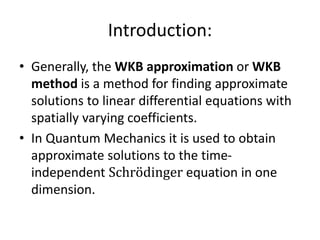
  • 1. Introduction: • Generally, the WKB approximation or WKB method is a method for finding approximate solutions to linear differential equations with spatially varying coefficients. • In Quantum Mechanics it is used to obtain approximate solutions to the time- independent Schrodinger equation in one dimension.
  • 2. Applications in Quantum Mechanics In quantum mechanics it is useful in 1. Calculating bound state energies (Whenever the particle cannot move to infinity) 2. Transmission probability through potential barriers. These are given in next slides.
  • 3. Main idea: • If potential 𝑽(𝒙) is constant and energy 𝐸 of the particle is 𝑬 > 𝑽, then the particle wave function has the form 𝜓 𝑥 = 𝐴𝑒±𝑖𝑘𝑥 where 𝑘 = √(2𝑚(𝐸−𝑉)) ℏ (+) sign indicates : particle travelling to right (-) sign indicates : particle travelling to left • General solution : Linear superposition of the two. • The wave function is oscillatory, with fixed wavelength, 𝜆 = 2𝜋 𝑘 . • The amplitude (A) is fixed.
  • 4. • If V (x) is not constant, but varies slow in comparison with the wavelength λ in a way that it is essentially constant over many λ, then the wave function is practically sinusoidal, but wavelength and amplitude slowly change with x. This is the inspiration behind WKB approximation. In effect, it identifies two different levels of x-dependence :- rapid oscillations, modulated by gradual variation in amplitude and wavelength.
  • 5. • If E<V and V is constant, then wave function is 𝜓 𝑥 = 𝐴𝑒±𝜅𝑥 where κ = √(2𝑚(𝑉−𝐸)) ℏ If 𝑽(𝒙) is not constant, but varies slowly in comparison with 1 𝜅 , the solution remain practically exponential, except that 𝐴 and 𝜅 are now slowly-varying function of 𝑥.
  • 6. Failure of this idea There is one place where this whole program is bound to fail, and that is in the immediate vicinity of a classical turning point, where 𝐸 ≈ 𝑉. For here 𝜆(𝑜𝑟 1 𝜅)) goes to infinity and 𝑉(𝑥) can hardly be said to vary “slowly” in comparison. A proper handling of the turning points is the most difficult aspect of the WKB approximation, though the final results are simple to state and easy to implement. The diagram showing turning points is given in next slide.
  • 8. The Classical Region • Let's now solve the Schrödinger equation using WKB approximation −ℏ2 2𝑚 𝑑2 𝜓 𝑑𝑥2 + 𝑉 𝑥 𝜓 = 𝐸𝜓 can be rewritten in the following way: 𝑑2 𝜓 𝑑𝑥2 = − 𝑝2 ℏ2 𝜓 ; 𝑝 𝑥 = 2𝑚(𝐸 − 𝑉(𝑥)) is the classical formula for the momentum of a particle with total energy 𝐸 and potential energy 𝑉(𝑥). Let’s assume 𝐸 > 𝑉(𝑥), so that 𝑝(𝑥) is real. This is the classical region , as classically the particle is confined to this range of 𝑥. The classical and non-classical region is shown in the diagram on the next slide.
  • 9. The WKB approximation V(x) E Classical region (E>V) Non-classical region (E<V) Fig: Classically, the particle is confined to the region where 𝑬 ≥ 𝑽(𝒙)
  • 10. The function 𝜓 In general, 𝜓 is some complex function; we can express it in terms of its amplitude 𝐴(𝑥), and its phase, 𝜙(𝑥) – both of which are real : 𝜓 𝑥 = 𝐴(𝑥)𝑒 𝑖𝜙(𝑥)
  • 11. Solving the Schrödinger equation 𝜓 𝑥 = 𝐴(𝑥)𝑒 𝑖𝜙(𝑥) Using prime to denote the derivative with respect to 𝑥, we find: 𝑑𝜓 𝑑𝑥 = (𝐴′+𝑖𝐴𝜙′)𝑒 𝑖𝜙 and 𝑑2 𝜓 𝑑𝑥2 = [𝐴′′ +2𝑖𝐴′ 𝜙′ + 𝑖𝐴𝜙′′ − 𝐴 𝜙′ 2 ]𝑒 𝑖𝜙 Putting all these into 𝑑2 𝜓 𝑑𝑥2 = − 𝑝2 ℏ2 𝜓 (From Schrödinger equation ) , we get
  • 12. 𝐴′′ + 2𝑖𝐴′ 𝜙′ + 𝑖𝐴𝜙′′ − 𝐴 𝜙′ 2 = − 𝑝2 ℏ2 𝐴 Solving for real and imaginary parts we get, 𝐴′′ − 𝐴 𝜙′ 2 = − 𝑝2 ℏ2 𝐴 𝐴′′ = 𝐴 (∅′)2− 𝑝2 ℏ2 𝐴′′ 𝐴 = (∅′)2− 𝑝2 ℏ2 The above equation cannot be solved in general, so we use WKB approximation: we assume amplitude A varies slowly, so that the A’’ term is negligible. We assume that 𝐴′′ 𝐴 << [(∅′)2− 𝑝2 ℏ2]. Therefore, we drop that part and we get 𝜙 𝑥 = ± 1 ℏ 𝑝 𝑥 𝑑𝑥
  • 13. And from second equation, we get 2𝐴′ 𝜙′ + 𝐴𝜙′′ = 0 𝐴2 𝜙′ ′ = 0 𝐴 = 𝐶 𝜙′ Where C is real constant.
  • 14. Thus from the previous slides from the equations and making ‘C’ a complex constant, we get 𝜓(𝑥) ≅ 𝐶 𝑝(𝑥) 𝑒± 𝑖 ℏ 𝑝 𝑥 𝑑𝑥 And the general solution can be written as 𝜓(𝑥) ≅ 1 𝑝(𝑥) 𝐶1 𝑒 𝑖 ℏ 𝑝 𝑥 𝑑𝑥 + 𝐶2 𝑒 −𝑖 ℏ 𝑝 𝑥 𝑑𝑥 where 𝐶1 and 𝐶2 are constants.
  • 15. Alternate approach In this approach, the wave function is expanded in powers of ℏ . Let, the wave function be: 𝜓 = 𝐴𝑒 𝑖 ℏ 𝑆(𝑥) Using this in: 𝑑2 𝜓 𝑑𝑥2 + 𝑘2 𝜓 = 0, we get 𝑑𝑆 𝑑𝑥 2 − 𝑖ℏ 𝑑2 𝑆 𝑑𝑥2 − 𝑘2 ℏ2 = 0 --------(1) Expanding S(x) in powers of ℏ2 : 𝑆 𝑥 = 𝑆0 𝑥 + 𝑆1 𝑥 ℏ + 𝑆2 𝑥 ℏ2 2 + ⋯
  • 16. ∴ 1 ⟹ 𝑑𝑆0 𝑑𝑥 2 − 𝑘2 ℏ 2 + 2 𝑑𝑆0 𝑑𝑥 𝑑𝑆1 𝑑𝑥 − 𝑖 𝑑2 𝑆0 𝑑𝑥2 ℏ = 0 ; (neglecting higher powers of ℏ). where 𝑘2 ℏ 2 = 2𝑚[𝐸 − 𝑉(𝑥)] For the above equation to be valid, the coefficient of each power of ℏ must vanish separately, 𝑑𝑆0 𝑑𝑥 2 − 𝑘2 ℏ 2 = 0 𝑜𝑟 𝑑𝑆0 𝑑𝑥 = ±𝑘ℏ ⟹ 𝑆0 x = ± 𝑘ℏ𝑑𝑥
  • 17. and, 2 𝑑𝑆0 𝑑𝑥 𝑑𝑆1 𝑑𝑥 − 𝑖 𝑑2 𝑆0 𝑑𝑥2 = 0 𝑜𝑟, 𝑑𝑆1 𝑑𝑥 = 𝑖 2𝑘 𝑑𝑘 𝑑𝑥 ; using the value of 𝑆0(x) 𝑜𝑟, 𝑆1 = 𝑖 2 𝑙𝑛𝑘 or, 𝑒 𝑖𝑆1 = 𝑘−1 2 ∴ 𝜓 = 𝐴𝑒 𝑖 ℏ 𝑆(𝑥) = 𝐴𝑒 𝑖 ℏ 𝑆0(𝑥)+𝑆1(𝑥)ℏ = 𝐴𝑒 𝑖 ℏ 𝑆0 𝑒 𝑖𝑆1 = 𝐴 1 𝑘 𝑒±𝑖 𝑘𝑑𝑥 𝑜𝑟 𝜓 = 𝐴 𝑘 𝑒±𝑖 𝑘𝑑𝑥 where A is a normalization constant.
  • 18. For 𝐸 < 𝑉 𝑥 : the Schrodinger equation is , 𝑑2 𝜓 𝑑𝑥2 − 𝜅2 𝜓 = 0 ; 𝜅2 = 2𝑚[𝑉 𝑥 −𝐸] ℏ2 Proceeding in a similar fashion , the solution can be obtained as 𝜓 = 𝐵 𝜅 exp(± 𝜅𝑑𝑥) ; where B is a normalization constant.
  • 19. Validity of WKB solution The zeroeth order WKB solution is: 𝜓0 𝑥 = 𝐴𝑒±𝑖 𝑥 𝑘 𝑥 𝑑𝑥 𝑜𝑟, 𝜓0 𝑥 = 𝐴𝑒 𝑖 𝑥 𝑘 𝑥 𝑑𝑥 ; considering positive part only. 𝑑𝜓0(𝑥) 𝑑𝑥 = 𝑖𝑘(𝑥)𝜓0(𝑥) 𝑜𝑟, 𝑑2 𝜓0 𝑑𝑥2 = 𝑖 𝑑𝑘 𝑑𝑥 𝜓0 + (𝑖𝑘)2 𝜓0 𝑜𝑟, 𝑑2 𝜓0 𝑑𝑥2 + 𝑘2 + 𝑖 𝑑𝑘 𝑑𝑥 𝜓0 = 0
  • 20. But we are interested in solving the following eqn. 𝑑2 𝜓0 𝑑𝑥2 + 𝑘2 𝜓0 = 0 Hence, 𝑑𝑘 𝑑𝑥 << 𝑘2 ⟹ 1 𝑘 𝑑𝑘 𝑑𝑥 ≪ 𝑘(𝑥) i.e. k(x) should not vary so rapidly This is the Validity condition for WKB approximation.
  • 21. The WKB approximation V(x) E Classical region (E>V) Non-classical region (E<V) Non-classical region (E<V) Turning points
  • 22. The WKB approximation  E V x   ( ) ( ) i p x dx WKB C x e p x    h  E V x Excluding the turning points:   1 ( ) ( ) p x dx WKB C x e p x    h
  • 23. Patching region The WKB approximation V(x) E Classical region (E>V) Non-classical region (E<V)   ( ) ( ) i p x dxC x e p x    h   1 ( ) ( ) p x dxD x e p x    h
  • 24. Connection Formulae 𝑘2 (𝑥) 𝑥 WKB soln not valid a Trigonometric WKB soln Exponential WKB soln Turning point Barrier to the right of turning point
  • 25. Barrier to the right of turning point 1 𝑘 exp[− 𝑥 𝑎 𝑘𝑑𝑥] → 2 𝑘 sin[ 𝑎 𝑥 𝑘𝑑𝑥 + 𝜋 4 ] And, 1 𝑘 exp[+ 𝑥 𝑎 𝑘𝑑𝑥] → 1 𝑘 cos[ 𝑎 𝑥 𝑘𝑑𝑥 + 𝜋 4 ]
  • 26. Barrier to the left of turning point WKB soln not valid 𝑘2 (𝑥) 𝑥 Trigonometric WKB soln Exponential WKB soln b Turning point
  • 27. Barrier to the left of turning point 2 𝑘 sin 𝑥 𝑏 𝑘𝑑𝑥 + 𝜋 4 → 1 𝑘 𝑒𝑥𝑝 − 𝑏 𝑥 𝑘𝑑𝑥 And, 1 𝑘 𝑐𝑜𝑠 𝑥 𝑏 𝑘𝑑𝑥 + 𝜋 4 → 1 𝑘 𝑒𝑥𝑝 + 𝑏 𝑥 𝑘𝑑𝑥
  • 29. Example 1 Potential Square well with a Bumpy Surface
  • 30. Potential Square well with a Bumpy Surface Suppose we have an infinite square well with a bumpy bottom as shown in figure: and 𝑉 𝑥 = 𝑠𝑜𝑚𝑒 𝑠𝑝𝑒𝑐𝑖𝑓𝑖𝑒𝑑 𝑓𝑢𝑛𝑐𝑡𝑖𝑜𝑛, 𝑖𝑓 0 < 𝑥 < 𝑎 ∞, 𝑜𝑡ℎ𝑒𝑟𝑤𝑖𝑠𝑒 𝑽 𝒙 𝒙𝟎
  • 31. Inside the well, (𝑎𝑠𝑠𝑢𝑚𝑖𝑛𝑔 𝐸 > 𝑉 𝑥 𝑡ℎ𝑟𝑜𝑢𝑔ℎ𝑜𝑢𝑡), we have or, 𝜓 𝑥 ≅ 1 𝑝(𝑥) 𝐶1 𝑠𝑖𝑛 1 ℏ 0 𝑥 𝑝 𝑥 𝑑𝑥 + 𝐶2 𝑐𝑜𝑠 1 ℏ 0 𝑥 𝑝 𝑥 𝑑𝑥 𝜓(𝑥) must go to zero at 𝑥 = 0 and 𝑥 = 𝑎. So, putting the values we get respectively, 𝐶2 = 0 and 0 𝑎 𝑝 𝑥 𝑑𝑥 = 𝑛𝜋 ℏ ,this quantization condition determines the allowed energies. 𝜓(𝑥) ≅ 1 𝑝(𝑥) 𝐶1 𝑒 𝑖 ℏ 0 𝑥 𝑝 𝑥 𝑑𝑥 + 𝐶2 𝑒 −𝑖 ℏ 0 𝑥 𝑝 𝑥 𝑑𝑥
  • 32. Special Case: If the well has a flat bottom i.e. (𝑉 𝑥 = 0), then 𝑝 𝑥 = 2𝑚𝐸 and from quantization equation, we get 𝑝𝑎 = 𝑛𝜋ℏ. Solving these, we get value of : 𝐸 𝑛 = 𝑛2 𝜋2ℏ2 2𝑚𝑎2 which is the formula for the discrete energy levels of the infinite square well.
  • 34. In the non-classical region (𝐸 < 𝑉), 𝜓(𝑥) ≅ 𝐶 𝑝(𝑥) 𝑒± 1 ℏ 0 𝑥 𝑝(𝑥) 𝑑𝑥 ; 𝑝(𝑥) is complex Let us consider the following example : problem of scattering from a rectangular barrier also called tunneling.
  • 35. To the left of the barrier (𝑥 < 0), 𝜓 𝑥 = 𝐴𝑒 𝑖𝑘𝑥 + 𝐵𝑒−𝑖𝑘𝑥 where 𝐴 is the incident amplitude and 𝐵 is the reflected amplitude, and 𝑘 = 2𝑚𝐸 ℏ . To the right of the barrier (𝑥 > 𝑎), 𝜓 𝑥 = 𝐹𝑒 𝑖𝑘𝑥 where 𝐹 is the transmitted amplitude. In the tunneling region (0 ≤ 𝑥 ≤ 𝑎) WKB approximation gives, 𝜓 𝑥 ≅ 𝐶 𝑝 𝑥 𝑒 1 ℏ 0 𝑥 𝑝 𝑥 𝑑𝑥 + 𝐷 𝑝(𝑥) 𝑒 −1 ℏ 0 𝑥 𝑝(𝑥) 𝑑𝑥
  • 36. The transmission probability is 𝑇 = 𝐹 2 𝐴 2 ∵ 𝐹 𝐴 ~ 𝑒− 1 ℎ 0 𝑎 𝑝 𝑥 𝑑𝑥 ∴ 𝑇 ≅ 𝑒− 2 ℎ 0 𝑎 𝑝 𝑥 𝑑𝑥 where T is transmission probability.
  • 37. Example 3 Eigen value equation for Bound State
  • 38. Eigen value equation for Bound State Here, a and b are the classical turning points. 𝜓𝐼 = 𝐴 𝜅 𝑒− 𝑥 𝑏 𝜅 𝑥 𝑑𝑥 ; 𝜅2 = −𝑘2 = 2𝑚 ℏ2 𝑉 𝑥 − 𝐸 Using connection formula at 𝑥 = 𝑎 𝜓𝐼𝐼 = 2𝐴 𝑘 𝑠𝑖𝑛 𝑎 𝑥 𝑘(𝑥)𝑑𝑥 + 𝜋 4
  • 39. For 𝑥 = 𝑏: 𝑎 𝑥 𝑘(𝑥)𝑑𝑥 + 𝜋 4 = 𝑎 𝑏 𝑘𝑑𝑥 − 𝑥 𝑏 𝑘𝑑𝑥 + 𝜋 4 + 𝜋 2 = 𝜋 2 + 𝜃 − 𝑥 𝑏 𝑘𝑑𝑥 + 𝜋 4 ∴ 𝑠𝑖𝑛 𝑎 𝑥 𝑘(𝑥)𝑑𝑥 + 𝜋 4 = 𝑐𝑜𝑠 𝜃 − 𝑥 𝑏 𝑘𝑑𝑥 + 𝜋 4 ∴ 𝜓𝐼𝐼 = 2𝐴 𝑘 𝑐𝑜𝑠 𝜃 − 𝑥 𝑏 𝑘𝑑𝑥 + 𝜋 4
  • 41. 𝜃 = 𝑛 + 1 2 𝜋 ; 𝑛 = 0,1,2,3 … 𝑎 𝑏 𝑘𝑑𝑥 = 𝑛 + 1 2 𝜋 This is the Eigen value equation for bound state using WKB approximation. Now, using this equation the energy Eigen values for Linear Harmonic Oscillator (LHO) can be calculated as shown in next slide :
  • 42. LHO energy Eigen values For LHO potential is 𝑉 𝑥 = 1 2 𝑚𝜔2 𝑥2 ∴ 𝑘2 𝑥 = 2𝑚 ℏ2 𝐸 − 1 2 𝑚𝜔2 𝑥2 = 2𝑚 ℏ2 1 2 𝑚𝜔2 𝑥0 2 − 𝑥2 where, 𝑥0 2 = 2𝐸 𝑚𝜔2 is the classical amplitude or turning points.
  • 43. 𝑜𝑟, 𝑘2 𝑥 = 𝑚2 𝜔2 ℏ2 𝑥0 2 − 𝑥2 Using this value of 𝑘(𝑥) in Eigen value equation for bound state, −𝑥0 +𝑥0 𝑚𝜔 ℏ 𝑥0 2 − 𝑥2 𝑑𝑥 = (𝑛 + 1 2 )𝜋 On solving the above equation, 𝐸 ℏ𝜔 = (𝑛 + 1 2 ) or, 𝐸 𝑛 = (𝑛 + 1 2 )ℏ𝜔 ; 𝑛 = 0,1,2, … - which are the energy Eigen values for a Linear Harmonic Oscillator.