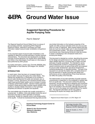
1. 1
EPA/540/S-93/503
February 1993
United States
Environmental Protection
Agency
Office of Solid Waste
and Emergency
Response
Office of
Research and
Development
Ground Water Issue
Suggested Operating Procedures for
Aquifer Pumping Tests
Robert S. Kerr Environmental
Research Laboratory
Ada, Oklahoma
Superfund Technology Support Center for
Ground Water
Paul S. Osborne*
Technology Innovation Office
Office of Solid Waste and Emergency
Response, US EPA, Washington, DC
Walter W. Kovalick, Jr., Ph.D.
Director
The Regional Superfund Ground Water Forum is a group of
ground-water scientists, representing EPA's Regional
Superfund Offices, organized to exchange up-to-date
information related to ground water remediation at Superfund
sites.
A very important aspect of ground water remediation is the
capability to determine accurate estimates of aquifer hydraulic
characteristics. This document was developed to provide an
overview of all the elements of an aquifer test to assist RPMs
and OSCs in the initial design of such tests or in the review of
tests performed by other groups.
For further information, contact Jerry Thornhill, RSKERL-Ada,
405/436-8604 or Paul Osborne, EPA Region VIII, 303/293-
1418.
INTRODUCTION
In recent years, there has been an increased interest in
ground water resources throughout the United States. This
interest has resulted from a combination of an increase in
ground water development for public and domestic use; an
increase in mining, agricultural, and industrial activities which
might impact ground water quality; and an increase in studies
of already contaminated aquifers. Decision-making agencies
involved in these ground water activities require studies of the
aquifers to develop reliable information on the hydrologic
properties and behavior of aquifers and aquitards.
The most reliable type of aquifer test usually conducted is a
pumping test. In addition, some site studies involve the use of
short term slug tests to obtain estimates of hydraulic
conductivity, usually for a specific zone or very limited portion
of the aquifer. It should be emphasized that slug tests provide
very limited information on the hydraulic properties of the
aquifer and often produce estimates which are only accurate
within an order of magnitude. Many experts believe that slug
tests are much too heavily relied upon in site characterization
and contamination studies. This group of professionals
recommends use of slug testing during the initial site studies
to assist in developing a site conceptual model and in
pumping test design.
This document is intended as a primer, describing the process
for the design and performance of an “aquifer test” (how to
obtain reliable data from a pumping test) to obtain accurate
estimates of aquifer parameters. It is intended for use by
those professionals involved in characterizing sites which
require corrective action as well as those which are proposed
for ground water development, agricultural development,
industrial development, or disposal activities. The goal of the
document is to provide the reader with a complete picture of
all of the elements of aquifer (pumping) test design and
performance and an understanding of how those elements
can affect the quality of the final data.
The determination of accurate estimates of aquifer hydraulic
characteristics is dependent on the availability of reliable data
from an aquifer test. This document outlines the planning,
equipment, and test procedures for designing and conducting
an accurate aquifer test. The design and operation of a slug
test is not included in this document, although slug tests are
often run prior to the design and implementation of an aquifer
test. The slug test information can be very useful in
developing the aquifer test design (see ASTM D-18
* Regional Ground Water Expert, U.S. EPA, Region VIII

2. 2
Committee, D4050 and D4104). If an accurate conceptual
model of the site is developed and the proper equipment, wells,
and procedures are selected during the design phase, the
resulting data should be reliable. The aquifer estimates
obtained from analyzing the data will, of course, depend on the
method of analysis.
This document is not intended to be an overview of aquifer
test analysis. The analysis and evaluation of pumping test
data is adequately covered by numerous texts on the subject
(Dawson and Istok, 1991; Kruseman and de Ridder, 1991;
Walton, 1962; and Ferris, Knowles, Brown, and Stallman,
1962). It should be emphasized, however, that information on
the methods for analyzing test data should be reviewed in
detail during the planning phase. This is especially important
for determining the number, location, and construction details
for all wells involved in the test.
A simple “pump” (specific capacity) test involves the pumping
of a single well with no associated observation wells. The
purpose of a pump test is to obtain information on well yield,
observed drawdown, pump efficiency, and calculated specific
capacity. The information is used mainly for developing the
final design of the pump facility and water delivery system.
The pump test usually has a duration of 2 to 12 hours with
periodic water level and discharge measurements. The pump
is generally allowed to run at maximum capacity with little or
no attempt to maintain constant discharge. Discharge
variations are often as high as 50 percent. Short-term pump
tests with poor control of discharge are not suitable for
estimating parameters needed for adequate aquifer
characterization. If the pump test is, however, run in such a
way that the discharge rate varies less than 5 percent and
water levels are measured frequently, the test data can also
be used to obtain some reliable estimates of aquifer
performance. It should be emphasized that an estimate of
aquifer transmissivity obtained in this manner will not be as
accurate as that obtained using an aquifer test including
observation wells.
By controlling the discharge variation and pumping for a
sufficient duration, it is possible to obtain reliable estimates of
transmissivity using water level data obtained during the pump
test. However, this method does not provide information on
boundaries, storativity, leaky aquifers, and other information
needed to adequately characterize the hydrology of an
aquifer. For the purpose of this document, an aquifer test is
defined as a controlled field experiment using a discharging
(control) well and at least one observation well.
The aquifer test is accomplished by applying a known stress
to an aquifer of known or assumed dimensions and observing
the water level response over time. Hydraulic characteristics
which can be estimated, if the test is designed and
implemented properly, include the coefficient of storage,
specific yield, transmissivity, vertical and horizontal
permeability, and confining layer leakage. Depending on the
location of observation wells, it may be possible to determine
the location of aquifer boundaries. If measurements are made
on nearby springs, it may also be possible to determine the
impact of pumping on surface-water features.
TEST DESIGN
Adequate attention to the planning and design phase of the
aquifer pumping test will assure that the effort and expense of
conducting a test will produce useful results. Individuals
involved in designing an aquifer test should review the
relevant ASTM Standards relating to: 1) appropriate field
procedures for determining aquifer hydraulic properties
(D4050 and D4106); 2) selection of aquifer test method
(D4043); and 3) design and installation of ground water
monitoring wells (D5092). The relevant portions of these
standards should be incorporated into the design.
All available information regarding the aquifer and the site
should be collected and reviewed at the commencement of
the test design phase. This information will provide the basis
for development of a conceptual model of the site and for
selecting the final design. It is important that the geometry of
the site, location and depth of observation wells and
piezometers, and the pumping period agree with the
mathematical model to be used in the analysis of the data. A
test should be designed for the most important parameters to
be determined, and other parameters may have to be de-
emphasized.
Aquifer Data Needs
The initial element of the test design, formulating a
conceptual model of the site, involves the collection and
analysis of existing data regarding the aquifer and related
geologic and hydrologic units. All available information on the
aquifer itself, such as saturated thickness, locations of aquifer
boundaries, locations of springs, information on all on-site and
all nearby wells (construction, well logs, pumping schedules,
etc.), estimates of regional transmissivities, and other
pertinent data, should be collected. Detailed information
relating to the geology and hydrology is needed to formulate
the conceptual model and to determine which mathematical
model should be utilized to estimate the most important
parameters. It is also important to review various methods for
the analyses and evaluation of pumping test data (Ferris,
Knowles, Brown, and Stallman, 1962; Kruseman and De
Ridder, 1991; and Walton, 1962 and 1970). Information
relating to the various analytical methods and associated data
needs will assist the hydrologist in reviewing the existing data,
identifying gaps in information, and formulating a program for
filling any gaps that exist.
The conceptual model of the site should be prepared after
carrying out a detailed site visit and an evaluation of the
assembled information. The review of available records
should include files available from the U. S. Geological
Survey, appropriate state agencies, and information from local
drillers with experience in the area. Formulation of a
conceptual model should include a brief analysis of how the
local hydrology/geology fits into the regional hydrogeologic
setting.
Aquifer Location
The depth to, thickness of, areal extent of, and lithology of the
aquifer to be tested should be delineated, if possible.
Aquifer Boundaries
Nearby aquifer discontinuities caused by changes in lithology
or by incised streams and lakes should be mapped. All known
and suspected boundaries should be mapped such that

3. 3
After the process of developing the site model and
determining which analytical methods should be used, it is
possible to move to the final design stage. The final stage of
the design involves development of the key elements of the
aquifer test: 1) number and location of observation wells; 2)
design of observation wells; 3) approximate duration of the
test; and 4) discharge rate.
Design of Pumping Facility
There are seven principal elements to be considered during
the pumping facility design phase: 1) well construction; 2) the
well development procedure; 3) well access for water level
measurements; 4) a reliable power source; 5) the type of
pump; 6) the discharge-control and measurement equipment;
and 7) the method of water disposal. These elements are
discussed in the following sections.
Well Construction
The diameter, depth and position of all intervals open to the
aquifer in the pumping well should be known, as should total
depth. The diameter must be large enough to accommodate
a test pump and allow for water level measurements. All
openings to the aquifer(s) must be known and only those
openings located in the aquifer to be tested should be open to
the well during the testing. If the pumping well has to be
drilled, the type, size, and number of perforations should be
established using data from existing well logs and from the
information obtained during the drilling of the new well itself.
The screen or perforated interval should be designed to have
sufficient open area to minimize well losses caused by fluid
entry into the well (Campbell and Lehr, 1972; and Driscoll,
1986).
A well into an unconsolidated aquifer should be completed
with a filter pack in the annular space between the well screen
and the aquifer material. To design an adequate filter pack, it
is essential that the grain size makeup of the aquifer be
defined. This is generally done by running a sieve analysis of
the major lithologic units making up the aquifer. The sizing of
the filter pack will depend on the grain size distribution of the
aquifer material. The well screen size would be established
by the sizing of the chosen filter pack (Driscoll,1986). The
filter pack should extend at least one (1) foot above the top of
the well screen. A seal of bentonite pellets should be placed
on top of the filter pack. A minimum of three (3) feet of pellets
should be used. An annulus seal of cement and/or bentonite
grout should be placed on top of the bentonite pellets. The
well casing should be protected at the surface with a concrete
pad around the well to isolate the wellbore from surface runoff
(ASTM Committee D-18, D5092; and Barcelona, Gibb, and
Miller, 1983).
Well Development
Information on how the pumping well was constructed and
developed should be collected during the review of existing
site information. It may be necessary to interview the driller. If
the well has not been adequately developed, the data
collected from the well may not be representative of the
aquifer. For instance, the efficiency of the well may be
reduced, thereby causing increased drawdown in the pumping
well. When a well is pumped, there are two components of
observation wells can be placed (chosen) where they will
provide the best opportunity to measure the aquifer’s
response to the pumping and the boundary effects during the
pumping test.
Hydraulic Properties
Estimates of all pertinent hydraulic properties of the aquifers
and pertinent geologic units must be made by any means
feasible. Estimates of transmissivity and the storage
coefficient should be made, and if leaky confining beds are
detected, leakage coefficients should be estimated. The
estimation of transmissivity and the storage coefficient should
be carried out by making a close examination of existing well
logs and core data in the area or by gathering information from
nearby aquifer tests, slug tests, or drill stem tests conducted
on the aquifer(s) in question. It may also be feasible to run a
slug test on the wells near the site to get preliminary values.
(See ASTM Committee D-18 Standards D4044 and D4104). It
should be noted that some investigators have found that slug
tests often produce results which are as much as an order of
magnitude low. Although some investigators have reported
results which are two orders of magnitude high because the
sand pack dominated the test. Such tests will, however,
provide a starting point for the design. If no core analyses are
available, the well log review should form a basis for utilizing
an available table which correlates the type of aquifer material
with the hydraulic conductivity. If detailed sample results from
drill holes are available and they have grain size analyses,
there are empirical formulas for estimation of transmissivity.
Estimation of storage coefficient is more difficult, but can be
based on the expected porosity of the material or the
expected confinement of the aquifer. It is recommended that
a range of values be chosen to provide a worst case and best
case scenario (Freeze and Cherry, 1979). Trial calculations of
well drawdown using these estimated values should be made
to finalize the design, location, and operation of test and
observation wells (Ferris and others, 1962; Campbell and
Lehr, 1972; and Stallman, 1971).
If local perched aquifers are of a significant size and
location to impact the pump test, this impact should be
estimated if possible. The final test design should include
adequate monitoring of any perched aquifers and leaky
confining beds. This might involve the placing of
piezometers into and/or above the leaky confining zone or
into the perched aquifer.
Evaluation of Existing Well Information
Because the drilling of new production wells and observation
wells expressly for an aquifer test can be expensive, it is
advisable to use existing wells for conducting an aquifer test
when possible. However, many existing wells are not suitable
for aquifer testing. They may be unsuitably constructed (such
as a well which is not completed in the same aquifer zone as
the pumping well) or may be inappropriately located. It is also
important to note that well logs and well completion data for
existing facilities are not always reliable. Existing data should
be verified whenever possible. The design of each well,
whether existing or to be drilled, must be carefully considered
to determine if it will meet the needs of the proposed test plan
and analytical methods. Special attention must be paid to well
location, the depth and interval of the well screen or
perforation, and the present condition of existing perforations.

4. 4
Water Level Measurement Access
It must be possible to measure depth to the water level in the
pumping well before, during, and after pumping. The quickest
and generally the most accurate means of measuring the
water levels in the pumped well during an aquifer test is to use
an electric sounder or pressure transducer system. The
transducer system may be expensive and may be difficult to
install in an existing well. It may be possible to run a 1/4 inch
copper line into the well as an air line. If the control well is
newly constructed, the continuous copper line should be
strapped to the pump column as it is being installed. If it is
correctly installed, an air line can be used with somewhat less
accuracy than an electric sounder or steel tape. An air line
with a bubbler and either a transducer or precision pressure
gage should be adequate for running an aquifer test.
With adequate temperature compensation, a surface mounted
pressure transducer is as precise as one that is submerged.
Steel tapes cannot always be used quickly enough in a
pumping well, except in wells with a small depth to water (less
than 100 feet) where the pump test crew has a fair amount of
experience and the well is modified for access of the steel
tape. Such modification often involves hanging a 3/4 inch pipe
in the well as access for the steel tape. The pipe should be
capped at the bottom with numerous 1/16 to 1/8 inch holes
drilled in the pipe and cap (especially needed for wells subject
to cascading water or surging). This will dampen water-level
surging caused by the pump and will eliminate the problems
caused by cascading water. In general, the use of a steel
tape is usually confined to the later stages of the pump test
where rapid changes in water levels are not occurring.
In cases where the pump is isolated by a packer to allow
production from a particular zone, a transducer system should
be used to monitor pumping hydraulic heads. It is important,
however, to calibrate the transducers before and after the test.
In addition, reference checks with an electric sounder or steel
tape should be made before, during, and after the test. The
ASTM Standard Test Method for determining subsurface liquid
levels in a borehole or monitoring well (D4750) should be
reviewed as part of the design process.
Reliable Power Source
Having power continuously available to the pump, for the
duration of the test, is crucial to the success of the test. If
power is interrupted during the test, it may be necessary to
terminate the test and allow for sufficient recovery so that pre-
pumping water-level trends can be extrapolated. At that point,
a new test would be run. If, however, brief interruptions in
power occur late in the test, the affect of the interruption can
be eliminated by pumping at a calculated higher rate for some
period so that the average rate remains unchanged. The
increased rate must be calculated such that the final portion of
the test compensates for the pumpage that would have
occurred during the interruption of pumping.
Pump Selection
A reliable pump is a necessity during an aquifer test. The
pump should be operated continuously during the test.
Should a pump fail during the pumping period of the test, the
time, effort, and expense of conducting the test could be
drawdown: 1) the head losses in the aquifer; and 2) the head
losses associated with entry into the well. A well which is
poorly constructed or has a plugged well screen will have a
high head loss associated with entry into the well. These
losses will affect the accuracy of the estimates of aquifer
hydraulic parameters made using data from that well. If the
well is suspected to have been poorly developed, or nothing is
known, it is advisable to run a step drawdown test on the well
to determine the extent of the problem. The step drawdown
test entails conducting three or more steps of increasing
discharge, producing drawdown curves such as shown in
Figure 1. The data provided by the step drawdown test
(multiple discharge test) can be analyzed using various
techniques (Rorabough, 1953; and Driscoll, 1986) to obtain an
estimate of well entry losses. If a determination is made that
plugging results in significant losses, the well should be
redeveloped prior to the pumping test using a surge block and/
or a pump until the well discharge is clear: i. e. the
development results in the well achieving acceptable turbidity
unit limits (Driscoll, 1986). In many cases, running a step
drawdown test to determine well efficiency after the well has
been surged is needed to assess the results of the
development process. The results of the post development
test should be compared with the step-drawdown test run prior
to development. This analysis will provide a means of
verifying the success of the well development.
Figure 1. Variation of discharge and drawdown in multiple
discharge tests (step drawdown tests).
Discharge-QDrawdown-Feet
Q2 ∆Q3
Q3 ∆Q4
Q4
∆Q2
∆Q1
Q1
t0 t1 t2 t3
∆s'
Time - Minutes
∆s''
∆s'''
∆s'
∆s''
∆s'''∆s''''

5. 5
rate is at least 20 percent more than the estimated long term
sustainable yield of the aquifer. The long term yield of the
aquifer should be determined by collecting data on pumping
rates in nearby wells. If possible, a short term test of one to
two hours should be run when the pump is installed. This test
data should be compared to the historic data as part of the
estimation process.
The pumping rate can be controlled by placing valves on the
discharge line and/or by placing controls on the pump power
source. A valve installed in the discharge line to create back
pressure provides effective control of the discharge rate while
conducting an aquifer test, especially when using an electric-
powered pump. A rheostatic control on the electric pump will
also allow accurate control of the discharge rate. When an
engine-powered pump is being utilized, installation of a
micrometer throttle adjustment device to accurately control
engine rpm is recommended in addition to a valve in the line.
Water Disposal
Discharging water immediately adjacent to the pumping well
can cause problems with the aquifer test, especially in tests of
permeable unconfined alluvial aquifers. The water becomes a
source of recharge which will affect the results of the test. It is
essential that the volumes of produced water, the storage
needs, the disposal alternatives, and the treatment needs be
assessed early in the planning process. The produced water
from the test well must be transported away from the control
well and observation wells so it cannot return to the aquifer
during the test. This may necessitate the laying of a
temporary pipeline (sprinkler irrigation line is often used) to
convey the discharge water a sufficient distance from the test
site. In some cases, it may be necessary to have on-site
storage, such as steel storage tanks or lined ponds. This is
especially critical when testing contaminated zones where
water treatment capacity is not available. The test designer
should carefully review applicable requirements of the RCRA
hazardous waste program, the underground injection control
program, and the surface water discharge program prior to
making decisions about this phase of the design. It may be
necessary to obtain permits for on-site storage and final
disposal of the contaminated fluids. Final disposal could
involve treatment and reinjection into the source aquifer or
appropriate treatment and discharge.
Design of Observation Well(s)
Verification of well response
As part of the process of selecting the location of the
observation wells needed for the chosen aquifer test design,
existing wells should be tested for their suitability as
observation wells. The existing information regarding well
construction should be reviewed as a screening mechanism
for identifying suitable candidates. The wells that are
identified as potential observation wells should be field tested
to verify that they are suitable for monitoring aquifer response.
The perforations or well screens of abandoned wells tend to
become restricted by the buildup of iron compounds,
carbonate compounds, sulfate compounds or bacterial growth
as a result of not pumping the well. Consequently, the
response test is one of the most important pre-pumping
examinations to be made if such wells are to be used for
observation (Stallman, 1971; and Black and Kip, 1977). The
wasted. Electrically powered pumps produce the most
constant discharge and are often recommended for use during
an aquifer test. However, in irrigation areas, line loads can
fluctuate greatly, causing variations in the pumping rate of
electric motors. Furthermore, electric motors are nearly
constant-load devices, so that as the lift increases (water level
declines), the pumping rate decreases. This is a particular
problem for inefficient wells or low transmissivity aquifers.
The discharge of engine-powered (usually gasoline or diesel)
pumps may vary greatly over a 24 hour period, requiring more
frequent monitoring of the discharge rate during the test. For
example, under extreme conditions a diesel-powered turbine
pump may have more than a 10 percent change in discharge
as a result of the daily variation in temperature. The change in
air temperature affects the combustion ratio of the engine
resulting in a variation in engine revolutions per minute (rpm).
The greater the daily temperature range,the greater the range
in engine rpm. Variations in barometric pressure may also
affect the engine operation and resulting rpm. Running the
engine at full throttle will reduce operational flexibility for
adjusting engine rpm and the resulting discharge. In areas
where outside temperatures are extreme, such as the desert
or a very cold region, it may be advisable to undertake
measures to prevent the engine from overheating or freezing.
In order to obtain good data during the period of recovery at
the end of pumping, it is necessary to have a check valve
installed at the base of the pump column pipe in the
discharging well. This will prevent the back flow of water from
the column pipe into the well when the pumping portion of the
test is terminated and the recovery begins. Any back flow into
the well will interfere with or totally mask the water level
recovery of the aquifer and this would make any aquifer
analysis based on recovery data useless or, at best,
questionable (Schafer, 1978).
Discharge-Control and Measurement Equipment
The well bore and discharge lines should be accessible for
installing discharge control and monitoring equipment. When
considering an existing well for the test well to be pumped
(control well), the well must either already be equipped with
discharge measuring and regulating equipment, or the well
must have been constructed such that the necessary
equipment can be added.
Control of the pumping rate during the test requires an
accurate means for measuring the discharge of the pump and
a convenient means of adjusting the rate to keep it as nearly
constant as possible. Common methods of measuring well
discharge include the use of an orifice plate and manometer,
an inline flow meter, an inline calibrated pitot tube, a calibrated
weir or flume, or, for low discharge rates, observing the length
of time taken for the discharging water to fill a container of
known volume (e.g. 5 gallon bucket; 55 gallon drum).
In addition to the potentially large variation in discharge
associated with the pump motor or engine, the discharge rate
is also related to the drop in water level near the pumping well
during the aquifer test. As the pumping lift increases, the rate
of discharge at a given level of power (such as engine rpm)
will decrease. The pump should not be operated at its
maximum rate. As a general rule, the pumping unit, including
the engine, should be designed so that the maximum pumping

6. 6
reaction of all wells to changing water levels should be tested
by injecting or removing a known volume of water into each
well and measuring the subsequent change of water level.
Any wells which appear to have poor response should be
either redeveloped, replaced, or dropped from consideration in
favor of another available well selected.
Total Depth
In general, observation wells should penetrate the tested
aquifer to the same stratigraphic horizon as the well screen or
perforated interval of the pumping well. This will require close
evaluation of logs to adjust for dipping formations. This
assumes the observation well is to be used for monitoring
response in the same aquifer from which the discharging well
is pumping. Actual screen design will depend on aquifer
geometry and site specific lithology. If the aquifer test is
designed to detect hydraulic connection between aquifers, one
observation well should be screened in the strata for which
hydraulic inter-connection is suspected. Depending on how
much information is needed, additional wells screened in other
strata may be needed (Bredehoeft and others, 1983; Walton,
1970; Dawson and Istok, 1991; and Hamlin, 1983).
Well Diameter
In general, observation well casing should have a diameter
just large enough to allow for accurate, rapid water level
measurements. A two-inch well casing is usually adequate for
use as an observation well in shallow aquifers which are less
than 100 feet in depth. They are, however, often difficult to
develop. A four- to six-inch diameter well will withstand a
more vigorous development process, and should have better
aquifer response when properly developed. Additionally, a
four or six inch diameter well may be required if a water-depth
recorder is planned, depending on the type of recording
equipment to be used. The difficulties in drilling a straight hole
usually dictate that a well over 200 feet deep be at least four
inches in diameter.
Well Construction
Ideally, the observation well(s) should have five to twenty feet
of perforated casing or well screen near the bottom of the well.
The final well screened interval(s) will depend on the nature of
geologic conditions at the site and the types of parameters to
be estimated. Any openings which allow water to enter the
well from aquifers which are not to be tested should be sealed
or closed off for the duration of the test. Ideally, the annular
space between the casing and the hole wall should be gravel
packed adjacent to the perforated interval to be tested. The
use of a filter pack in wells with more than one screened
interval will, however, create a problem. There is no reliable
method for sealing the annular space of any unwanted filter
packed interval even though the screen can be isolated. The
size of the filter material should be based on the grain size
distribution of the zone to be screened (preferably based on a
sieve analysis of the material). The screen size should be
determined based on the filter pack design (Driscoll, 1986).
The space above the gravel should be sealed with a sufficient
amount of bentonite or other grout to isolate the gravel pack
from vertical flow from above. If the bentonite does not extend
to the surface, it will be necessary to put a cement seal on top
of the bentonite prior to back filling the remaining annular
space. A concrete pad should be placed around the well to
prevent surface fluids from entering the annular material.
After installation is finished, the observation well should be
developed by surging with a block, and/or submersible pump
(Campbell and Lehr, 1972; and Driscoll, 1986) for a sufficient
period (usually several hours) to meet a pre-determined level
of turbidity.
Radial Distance and Location Relative to
the Pumped Well
If only one observation well is to be used, it is usually located
50 to 300 feet from the pumped well. However, each test
situation should be evaluated individually, because certain
hydraulic conditions may exist which warrant the use of a
closer or more distant observation well. If the test design
requires multiple observation wells, the wells are often placed
in a straight line or along rays that are perpendicular from the
pumping well. In the case of multiple boundaries or leaky
aquifers, the observation wells need to be located in a manner
which will identify the location and effect of the boundaries. If
the location of the boundary is suspected before the test, it is
desirable to locate most of the wells along a line parallel to the
boundary and running through the pumping well, as shown in
Figure 2. If aquifer anisotropy is expected, the observation
wells should be located in a pattern based on the suspected or
known anisotropic conditions at the site (Bentall and others,
1963; Ferris and others, 1962; Walton, 1962 and 1970; and
Dawson and Istok, 1991). If the principal directions of
anisotropy are known, drawdown data from two wells located
on different rays from the pumping well will be sufficient. If the
principal directions of anisotropy are not known, at least three
wells on different rays are needed.
FIELD PROCEDURES
Well thought out field procedures and accurate monitoring
equipment are the key to a successful aquifer test. The
following three sections provide an overview of the methods
and equipment for establishing a pre-test baseline condition
and running the test itself.
Necessary Equipment for Data Collection
During an aquifer test, equipment is needed to measure/
record water levels, well discharges, and the time since the
beginning of the test, and to record accumulated data.
Appendix One contains a detailed description of the types of
equipment commonly used during an aquifer test. Appendix
Two is an example form for recording test data.
Establish Baseline Trend
Collecting data on pre-test water levels is essential if the
analysis of the test data is to be completely successful. The
baseline data provides a basis for correcting the test data to
account for on-going regional water level changes. Although
the wells on-site are the main target for baseline
measurements, it is important to measure key wells adjacent
to the site and to account for off-site pumping which may
affect the test results.
Baseline water levels
Prior to beginning the test, it will be necessary to establish a

7. 7
#4 r4
200'
100' 200' 400'
r1 r2
r3
#1 #2 #3
r1-ir2-i
r3 -ir4 -i
230'±
P.W.
Edge of Valley Fill
Image
Well
Desolation Mtns
Approximate
Boundary of Buried Bedrock
Pediment
P.W. = pumping
or control well
Figure 2. Observation well/pumping well location to determine buried impermeable boundary.
baseline trend in the water levels in the pumping and all
observation wells. As a general rule, the period of observation
before the start of the test (t0
), should be at least one week.
Baseline measurements must be made for a period which is
sufficient to establish the pre-pumping water level trends on
site (see Figure 3). The baseline data must be sufficient to
explain any differences between individual observation wells.
As shown in Figure 3, the water levels in on-site wells were
declining prior to the test. The drawdown during the test must
be corrected to account for the pre-pumping trend.
Nearby pumping activities
During the baseline measurements, the on-off times should be
recorded for any nearby wells in use. The well discharge
rates should be noted as should any observed changes in the
proposed on-site control well and observation wells. Baseline
water level measurements should be made in all off-site wells
within the anticipated area of influence. As shown in Figure 3,
the baseline period should be sufficient to establish the pretest
pumping trends and to explain any differences in trends
between individual off-site wells.
Significant effects due to nearby pumping wells can often be
removed from the test data if the on-off times of the wells are
monitored before and during the test. Interference effects may
not, however, always be observable. In any case, changes
associated with nearby pumping wells will make analysis more
difficult. If possible, the cooperation of nearby well owners
should be obtained to either cease pumping prior to and
during the test period or to control the discharge of these wells
during the baseline and test period. The underlying principle
is to minimize changes in regional effects during the baseline,
test and recovery periods.
Barometric pressure changes
During the baseline trend observation period, it is desirable to
monitor and record the barometric pressure to a sensitivity of
plus or minus 0.01 inches of mercury. The monitoring should
continue throughout the test and for at least one day to a week
after the completion of the recovery measurement period.
This data, when combined with the water level trends
measured during the baseline period, can be used to correct
for the effects of barometric changes that may occur during
the test (Clark, 1967).
Local activities which may affect test
Changes in depth to water level, observed during the test,
may be due to several variables such as recharge, barometric
response, or “noise” resulting from operation of nearby wells,
or loading of the aquifer by trains or other surface
disturbances (King, 1982). It is important to identify all major
activities (especially cyclic activities) which may impact the
test data. Enough measurements have to be made to fully
characterize the pre-pumping trends of these activities. This
may necessitate the installation of recording equipment. A
summary of this information should be noted in the comments
section of the pumping test data forms.
Test Procedures
Initial water level measurements
Immediately before pumping is to begin, static water levels in
all test wells should be recorded. Measurements of drawdown
in the pumping well can be simplified by taping a calibrated
steel tape to the electric sounder wire. The zero point of the
tape may be taped at the point representing static water level.
This will enable the drawdown to be measured directly rather
than by depth to water.
Measuring water levels during test
If drawdown is expected in the observation well(s) soon after

8. 8
testing begins and continuous water level recorders are not
installed, an observer should be stationed at each observation
well to record water levels during the first two to three hours of
testing. Subsequently, a single observer is usually able to
record water levels in all wells because simultaneous
measurements are unnecessary. If there are numerous
observation wells, a pressure transducer/data-logging system
should be considered to reduce manpower needs.
Time frame for measuring water levels
Table 1 shows the recommended maximum time intervals for
recording water levels in the pumped well. NOTE: the times
provided in Table 1 are only the maximum recommended time
intervals--more frequent measurements may be taken if test
conditions warrant. For instance, it is recommended that
water level measurements be taken at least every 30 seconds
for the first several minutes of the test (see ASTM Committee
D-18, D 4050). Figure 4 is a hypothetical logarithmic plot of
drawdown versus time for an observation well. This plot
illustrates the need for the frequency of measurements given
in Table 1. As shown on the plot, frequent measurements
during early times are needed to define the drawdown curve.
The data used in Figure 4 was collected with a downhole
pressure transducer and electronic data recording equipment.
Thus, water levels could be collected about every 6 seconds
initially and less frequently as the test progresses. As time
since pumping started increases, the logarithmic scale
dictates that less frequent measurements are needed to
adequately define the curve.
Measurements in the observation well(s) should occur often
enough and soon enough after testing begins to avoid missing
the initial drawdown values. Actual timing will depend on the
aquifer and well conditions which vary from test area to test
area. Estimates for timing should be made during the
planning stages of aquifer testing using estimated aquifer
parameters based on the conceptual model of the site.
Table 1. Maximum Recommended Time Intervals
for Aquifer Test Water Level Measurements*
0 to 3 minutes ........................... every 30 seconds
3 to 15 minutes .................................every minute
15 to 60 minutes ......................... every 5 minutes
60 to 120 minutes ...................... every 10 minutes
120 min. to 10 hours ................. every 30 minutes
10 hours to 48 hours ..................... every 4 hours
48 hours to shut down .................. every 24 hours
* Dr. John Harshbarger, personal communication, 1968.
Monitoring discharge rate
During the initial hour of the aquifer test, well discharge in the
pumping well should be monitored and recorded as frequently
as practical. Ideally, the pretest discharge will equal zero. If it
does not, the discharge should be measured for the first time
within a minute or two after the pump is started.
It is important when starting a test to bring the discharge up to
the chosen rate as quickly as possible. How frequently the
discharge needs to be measured and adjusted for a test
depends on the pump, well, aquifer, and power
characteristics. Output from electrically driven equipment
requires less frequent adjustments than from all other
pumping equipment. Engine-driven pumps generally require
adjustments several times a day because of variation that
occurs in the motor performance due to a number of factors,
including air temperature effects. At a minimum, the
discharge should be checked four times per day: 1) early
Figure 3. Example test site showing baseline, pumping test, and recovery water level measurements in one of
the wells.
050
Observation
Well C
Observation
Well B
Observation Well A
Pumped Well
100
225 m
25
75 m
N
Map of Aquifer Test Site
Recovery period
6 7 8 9 10 11 12 13 14 15 16
12
11
10
9
8
7
6
5
4
3
Prepumping
period
Pumping
period
Drawdown(S)
Recovery
Regional trend
Pump on
Pump
off
Change of Water Level in Well B
Days Since Monitoring Commenced
DepthtoWater,inMeters
BelowMeasuringPoint
meters

9. 9
Figure 4. Logarithmic plot of s vs t for observation well.
Length of test
The amount of time the aquifer should be pumped depends on
the objectives of the test, the type of aquifer, location of
suspected boundaries, the degree of accuracy needed to
establish the storage coefficient and transmissivity, and the
rate of pumping. The test should continue until the data are
adequate to define the shape of the type curve sufficiently so
that the parameters required are defined. This may require
pumping for a significant period after the rate of water level
change becomes small (so called water level “stabilization”).
This is especially the case when the locations of boundaries or
the effects of delayed drainage are of interest. Their influence
may occur a few hours after pumping starts (see Figure 3), or
it may be days or weeks. Some aquifer tests may never
achieve equilibrium, or exhibit boundary effects.
Although it is not necessary for the pumping to continue until
equilibrium is approached, it is recommended that pumping be
continued for as long as possible and at least for 24 hours.
Recovery measurements should be made for a similar period
or until the projected pre-pumping water level trend has been
attained. The costs of running the pump a few extra hours are
low compared with the total costs of the test, and the
improvement in additional information gained could be the
difference between a conclusive and an inconclusive aquifer
test.
Water disposal
As discussed previously, the water being pumped must be
disposed of legally within applicable local, State, and Federal
morning (2 AM); 2) mid-morning (10 AM); 3) mid-afternoon (3
PM); and 4) early evening (8 PM). The discharge should
never be allowed to vary more than plus or minus 5 percent
(Ferris, J. G., personal communication, 1/19/68). The lower
the discharge rate, the more important it is to hold the
variation to less than 5 percent. The variation of discharge
rate has a large effect on permeability estimates calculated
using data collected during a test. The importance of
controlling the discharge rate can be demonstrated using a
sensitivity analysis of pumping test data. An analysis of this
type indicates that a 10 percent variation in discharge can
result in a 100 percent variation in the estimate of aquifer
transmissivity. Thus, short-term pumping tests with poor
control of discharge are not suitable for estimating parameters
needed for adequate site characterization. If, however, the
pumping test is run in such a way that the discharge rate
varies less than 5 percent and water levels are measured
frequently, the short-term pumping test data can be used to
obtain some reliable estimates of aquifer performance.
It should be emphasized, however, that some random, short-
term variations in discharge may be acceptable, if the average
discharge does not vary by more than plus or minus 5 percent.
A systematic or monotonic change in discharge (usually, a
decrease in discharge with increasing time) is, however,
unacceptable.
Water level recovery
Recovery measurements should be made in the same manner
as the drawdown measurements. After pumping is
terminated, recovery measurements should be taken at the
same frequency as the drawdown measurements listed above
in Table 1.
110 102 10310-1
10-1
1
10
s,inFeet
t, in Minutes

10. 10
rules and regulations. This is especially true if the ground
water is contaminated or is of poor quality compared to that at
the point of disposal. During the pumping test, the individuals
carrying out the test should carry out water quality monitoring
as required by the test plan and any necessary disposal
permits. This monitoring should include periodic checks to
assure that the water disposal procedures are following the
test design and are not recharging the aquifer in a manner that
would adversely affect the test results. The field notes for the
test should document when and how monitoring was
performed.
Recordkeeping
All data should be recorded on the forms prepared prior to
testing (See Appendix 2). An accurate recording of the time,
water level, and discharge measurements and comments
during the test will prove valuable and necessary during the
data analyses stage following the test.
Plotting data
During the test, a plot of drawdown versus time on semi-log
paper should always be prepared and updated as new data is
collected for each observation well. A plot of the data
prepared during the actual test is essential for monitoring the
status and effectiveness of the test. The plot of drawdown
versus time will reveal the effects of boundaries or other
hydraulic features if they are encountered during the test, and
will indicate when enough data for a solution have been
recorded. A semi-log or log-log mass plot of water level data
from all observation wells should be prepared as time allows.
Such a plot can be used to show when aquifer conditions are
beginning to affect individual wells. More importantly, it
enables the observer to identify erroneous data. This is
especially important if transducers are being used for data
collection. The utilization of a portable PC with a graphics
package is an option for use in carrying out additional field
manipulation of the data. It should not, however, be a
substitute for a manual plot of the data.
Precautions
(a) Care should be taken for all observers to use the same
measuring point on the top of the well casing for each
well. If it is necessary to change the measuring point
during the test, the time at which the point was changed
should be noted and the new measuring point described in
detail including the elevation of the new point.
(b) Regardless of the prescribed time interval, the actual time
of measurement should be recorded for all
measurements. It is recognized that the measurements
will not be taken at the exact time intervals suggested.
(c) If measurements in observation well(s) are taken by
several individuals during the early stages of testing, care
should be taken to synchronize stop watches to assure
that the time since pumping started is standardized.
(d) It is important to remember to start all stop watches at the
time pumping is started (or stopped if performing a
recovery test).
(e) Comments can be valuable in analyzing the data. It is
important to note any problems, or situations which may
alter the test data or the accuracy with which the observer
is working.
(f) If several sounders are to be used, they should be
compared before the start of the test to assure that
constant readings can be made. If the sounder in use is
changed, the change should be noted and the new
sounder identified in the notes.
PUMPING TEST DATA REDUCTION AND
PRESENTATION
All forms required for recording the test data should be
prepared prior to the start of the test and should be attached
to a clip board for ease of use in the field. It is an option to
have a portable PC located on-site with appropriate
spreadsheets and graphics package to allow for easier
manipulation of the data during the test. The hard copy of the
forms should be maintained for the files.
Tabular Data
All raw data in tabular form should be submitted along with the
analysis and computations. The data should clearly indicate
the well location(s), and date of test and type of test. All data
corrections, for pre-pumping trends, barometric pressure
fluctuations and other corrections should be given individually
and clearly labeled. All graphs used for corrections should be
referenced on the specific table. These graphs should be
attached to the data package.
Graphs
All graphs or plots should be drafted carefully so that the
individual points which reflect the measured data can be
retrieved. Semi-logarithmic and logarithmic data plots (see
Figures 5 and 6) should be on paper scaled appropriately for
the anticipated length of the test and the anticipated
drawdown. All X-Y coordinates shall be carefully labeled on
each plot. All plots must include the well location, date of test,
and an explanation of any points plotted or symbols used.
ANALYSIS OF TEST RESULTS
Data analysis involves using the raw field data to calculate
estimated values of hydraulic properties. If the design and
field-observation phases of the aquifer test are conducted
successfully, data analyses should be routine and successful.
The method(s) of analysis utilized will depend, of course, on
particular aquifer conditions in the area (known or assumed)
and the parameters to be estimated.
Calculations
All calculations and data analyses must accompany the final
report. All calculations should clearly show the data used for
input, the equations used and the results achieved. Any
assumptions made as part of the analysis should be noted in
the calculation section. This is especially important if the data
were corrected to account for barometric pressure changes,
off-site pumping changes, or other activities which have
affected the test. The calculations should reference the
appropriate tables and graphs used for a particular
calculation.

11. 11
Figure 6. Logarithmic plot of s vs t for Observation Well 23S/25E-17Q2
at Pixley, CA.
0
1
2
3
4
5
6
7
8
9
10
11
1 2 3 5 10 20 30 50 100 200 300 500
Time after pumping stopped, t, in minutes
Calculatedrecovery(s-s')infeet
∆s=5.2ft.
Joe's Garage
Peridot, AZ
Test
Oct 29-30, 1966
Time - Recovery Curve
Observation Well 1
T = 15,200 gal per day per ft
Av. pumping rate, Q = 300 gpm
T = =
264 Q
∆s
264 x 300
5.2
Figure 5. Time recovery curve for observation well - October 30, 1966.
Match Point
I/(uβ) = 1.0
I/u = 1.0
s = 5.3 ft.
t = 12.6 min
10 102 103 1041
10-2
10-1
1
10
s,infeet
t, in minutes

12. 12
Aquifer Test Results
The results of an aquifer pumping and recovery test should
be submitted in narrative format. The narrative report should
include the raw data in tabular form, the plots of the data, the
complete calculations and a summary of the results of the test.
The assumptions made in utilizing a particular method of
analysis should also be included.
SUMMARY-EXAMPLE FACILITY DESIGN
As a means of focusing the discussions presented in the
preceding sections, the following example of an aquifer
pumping test is described. The facility layout is shown in
Figure 7. The site is located near a normally dry river channel
which is subject to flood flows. The site was constructed for
the purpose of carrying out experiments relating to artificial
recharge of a shallow alluvial aquifer. The proposed methods
of recharge involved use of a pit and a well.
The aquifer at the site is comprised of unconsolidated basin fill
material, mainly silty sand and gravel with some clay lenses.
The depth to water is generally greater than 50 feet and the
river is a source of recharge when it flows. There are
extensive gravel lenses above the water table which outcrop
at the base of the river channel. These lenses occur beneath
the site.
Figure 7 shows the locations of the various monitoring wells
relative to the recharge facilities and the river. The well
locations were selected to facilitate both characterization of
the site and subsequent evaluation of the various recharge
tests. The recharge well (used as the pumping well during the
site aquifer tests) and the eight inch observation wells were
completed to a depth of 150 feet in the upper water bearing
unit of a basin fill aquifer. The depth to water in the area was
about 75 feet. The recharge and observation wells were
screened from about 80 feet to 140 feet. The 1-3/4 inch
access tubes were 80-100 feet deep with a five-foot well
screen on the bottom of each tube.
The eight-inch observation wells were placed in a line parallel
to the river to assess both the effect of flood flows on the
aquifer and the hydraulic characteristics of the recharge site
itself. The 1-3/4 inch access tubes were positioned for
monitoring ground-water movement near the top of the water
table in response to aquifer recharge and discharge (pumping)
tests. The two inch piezometers at varying depths were
constructed to evaluate shallow ground-water movement in
response to recharge.
Figure 8 is a plan view of the recharge facility showing the
pumping/recharge well and the water distribution system. The
pumping well was equipped with a downhole turbine pump
powered by a methane driven, 6-cylinder engine. As indicated
Figure 7. Recharge facility well layout.
0 10 20
5 15 25 50 100
low flow channel
located
300 ft from
recharge
well
- 8" observation well 150' deep
- 1 3/4" access tube 80'-100' deep
- 2" piezometer tube
River Bank (approximate)C
fence
fence
caretaker
area
fence
recharge pit
recharge well
9
8
C A 7 6 5 4
10 20 11
19
W-12.5 W-50 W-100
W-25 W-75
E-75 E-25
E-100 E-50 E-12.5

13. 13
on Figure 8, the pump discharge was measured using a
Parshall flume (see Figure 9). The water from pumping tests
was discharged off-site via the concrete box and distribution
line. To prevent interference with test results from nearby
recharge of the pumping test water, a temporary pipeline was
constructed from irrigation pipe. This temporary line ran from
the end of the river drain line to a point 1200 feet down stream
out of the estimated area of influence. The ground water was
not contaminated. Thus, special water quality monitoring was
not required.
The pumping tests for site characterization involved the
following monitoring procedure:
1. The eight-inch observation well closest to the
recharge well (Well A) was equipped with a Stevens
water stage recorder with an electric clock geared for
a 4-hour chart cycle;
2. The other two eight-inch observation wells (Wells B
and C) were equipped with Stevens water stage
recorders with an electric clock geared for a 12-hour
chart cycle;
3. The pumping well was equipped with a stilling well
composed of a 3/4-inch pipe strapped to the pump
column. The stilling well was drilled with 1/4-inch
holes through the length. The stilling well was used
for assessing the well for water level measurements
with a 150-foot steel tape. The steel tape was
marked in 0.01 ft. increments for the first 100 feet and
in 0.1 ft. increments for the remaining 50 feet;
4. The 1-3/4 inch access wells were monitored at least
once a day with a neutron moisture logger to assess
changes in saturation as the water level declined in
response to the test. This information was used to
verify the water level declines in the regular
monitoring wells and to aid in assessing the delayed
drainage effects which were to be estimated using the
water level response data from the eight-inch
observation wells;
5. A continuous recording barograph was located in a
standard construction, USDA weather station shed
located between access Wells 9 and 10; and
6. The pump engine was equipped with an rpm gage to
monitor pump performance and a micrometer
adjustment on the throttle.
A step drawdown test and several short-term pumping tests
were run at the site prior to running the principal aquifer
characterization test. The step drawdown test was used as a
means of selecting the final pumping test design. The short
term tests were used to obtain an initial picture of aquifer
response.
The results of the step drawdown test run on the recharge well
after development indicated that the well was suitable for use
as a test well. The results of the step test were also used to
estimate well efficiency at different rates. Table 2 gives the
efficiencies for three (3) discharge rates. As indicated, the
well efficiency was greater than 90% for a rate of about 200
Figure 8. Water distribution and drainage facilities at the artificial recharge site.
Bank of River
Flow Meter Riser 8" Valve
Low Lift
Pump
Holding
Pond
Recharge Pit
103'45' 2' 169' 10'
150'
26'
Drain Line to
River
3' x 3' x 7' concrete
box
Distribution Line
8" K-M, A-C Class
1500 Sewer
Chainlink Fence
4" Steel
Line
By-Pass
Line
9" Parshall Flume
A-C Ditch Liner
Recharge Well

14. 14
Figure 9. Parshall flume dimensions.
gpm. Based on this data, the design rate for the long-term
test was set at about 200 gpm (actual average was 204 gpm).
Table 2. Well Efficiency of R#1 after 200 Minutes of Pumping
Discharge Theoretical Actual Well
Drawdown Drawdown Efficiency
gpm ft ft percent
189 7.00 7.51 92
326 11.88 14.71 81
474 17.27 25.41 68
Because the initial short-term tests indicated that delayed
drainage was an issue at the site, the main test was designed
to run for a continuous period of at least 20 days. The actual
scheduling of the test was established to try to avoid flow in
the river as a result of a major precipitation event during the
background, pumping, and recovery periods. The chosen test
period was in the fall after the end of the irrigation season,
which also minimized off-site pumping that might affect the
results. It should be noted that two short-term tests were
planned to follow the main pumping test during the winter
rainy season when flow in the river was possible. This was
done to allow the impacts of an uncontrolled recharge event
on the system to be assessed. The main pumping test would
provide a basis for comparison.
The discharging well was measured on a time schedule per
the criteria in Table 1, except that measurements for the initial
10 minute period were taken every 30 seconds. The
observation wells were observed manually on the same
schedule for the initial 30 minute period and then the
recorders were utilized. Discharge measurements were
monitored at least every 5 minutes for the first 30 minutes and
then were monitored with water levels for the first 12 hours.
Discharge measurements were monitored at least four times
daily until the end of the test. The access tubes were
monitored twice daily to assess changes in saturation near the
water table.
The results from the long term pumping test are shown on
Figure 10 as a semi-log data mass plot (drawdown versus log
time) of the data for the three (3) observation wells. The large
initial water level decline for Observation Well A is due to its
close proximity to the pumping well (15 feet). The rise in
water level at the end of the test was caused by a slight
decrease in discharge rate.
Values of T and S were obtained by the non-equilibrium
method. The plots of drawdown as a function of log time did
not give a good overlay on the non-equilibrium type curve for
early times. For later times, it was possible to obtain a good
match. The match points obtained for the three observation
wells are listed in Table 3. The values of T and S are also
shown in Table 3. As indicated, the estimates of T and S were
in close agreement.
H
b
Well
Gage
G
age
Direction
of Flow
2/3 A
A
D
W
C
LL
PLAN
B F G
Ha
Gage
Hb Gage K Q
E
Level Floor
Angle-Iron Crest
Slope 1/4
Y
X
N
Water Surface P
H
a
Well

15. 15
Well C
Well A
Well B
10.0
9.0
8.0
7.0
6.0
5.0
4.0
3.0
2.0
1.0
0.0
1 10 100 1,000 10,000
Drawdown-Feet
Time after Pumping Commenced - Minutes
Figure 10. Drawdown versus log of time in observation wells A, B, and C during pumping of R#1.
Table 3. Values of T and S Obtained by Non-Equilibrium Equation for Discharge Conditions.
Location w(u) l/u s t r T S
ft min ft gpd/ft
Well A 110 105
0.62 14900 14.7 37,600 0.01
Well B 1 10 0.62 1780 280.0 37,600 0.03
Well C 1 10 0.58 530 175.4 40,200 0.03
The estimates for storativity were also in reasonable
agreement. It is important to note that the test results
showed delayed drainage to be a significant factor at this
site. The initial estimates of storativity using data from the
early part of the test were about 1 x 10-5
rather than 3 x 10-2
estimated after 20 days of pumping. This effect was
expected because of the heterogeneous nature of the
basin fill. As a means of comparison, water balance
studies on a large well field located 15 miles away
(completed in the same material) were reviewed. These
studies provided an estimate of storage coefficient (based
on 10 years of pumpage) of about 0.15. Thus, it was
concluded that the aquifer at the site was under water table
conditions, but significant delayed drainage effects were
present.
The results of the pumping tests at the site were used to
characterize the site and design several long-term
recharge experiments. This included monitoring design for
evaluation of the effect of river flows on the regional
aquifer.

16. 16
anticipated. If rapid drawdown, cascading water,
or high frequency oscillation are anticipated,
electric sounders, float actuated recorders or
pressure transducers are preferred.
(b) Steel tapes are not recommended for use in the
pumping well because of fluctuating water levels
caused by the pump action, possible cascading
water and the necessity for obtaining rapid water
level measurements during the early portions of
the aquifer pumping and recovery tests. If tapes
are used, and the water level fluctuates, the well
must be equipped with a means of dampening
fluctuating water levels. Additional manpower
will be needed during the initial stages of the
test.
(4) Pressure Transducers
Pressure transducers are often used in situations
where access to the well is restricted, such as a well
where packers are being used to isolate a certain
zone. They may also be applicable in large-scale
tests using a computerized data collection system.
Such a system will significantly reduce the manpower
needed during the initial stages of a multiple well test.
The most common installation uses down hole
transducers with recording of the results taking place
on the surface.
(a) Transducers should be calibrated prior to
installation, and should be capable of accurately
detecting changes of less than .005 psi.
Transducer systems which will accurately record
water level changes of .001 feet are available.
The resolution of transducers, however, depends
on the full scale range. Where large drawdowns
are expected, such resolution is not possible.
(b) After installation, the transducers and recording
equipment should be calibrated by comparing
pressure readings to actual water level
measurements taken with a steel tape. Periodic
measurements of the water level should be
made during the test to verify that the
transducers are functioning properly.
(c) The effect of barometric changes on the
transducers should be determined prior to
and during the test. This will require
continuous monitoring of the barometric
pressure at the site as well as periodic
comparisons of water level and transducer
readings (Clark, 1967).
b. Discharge Measurement
The equipment commonly used for measuring discharge
in the pumping well includes orifice plates, in-line water
meters, Parshall flumes and recorders, V-notch weirs, or,
for low discharge rates, a container of known volume, and
a stop watch (Driscoll, 1986). The choice of method will
depend upon a combination of factors, including i)
accuracy needed, ii) planned discharge rate, iii) facility
layout, and iv) point of discharge. If, for instance, it is
Appendix One
Equipment for Data Collection
a. Water Levels
Water level measurements can be made with electric
sounders, air line and pressure gages, calibrated steel
tapes, or pressure transducers (Garber and Koopman,
1968; and Bentall and others, 1963).
(1) Electric Sounders
(a) An electric sounder is recommended for
measuring water levels in the pumping well
because it will allow for rapid, multiple water
level readings, especially important during the
early stages of aquifer pumping and recovery
tests.
(b) A dedicated sounder should be assigned to each
observation well throughout the duration of the
test. This is particularly important in ground-
water quality studies to prevent cross
contamination.
(c) Each sounder should be calibrated prior to the
commencement of testing to assure accurate
readings during the test.
(2) Air Lines and Pressure Gages
(a) Air lines are only recommended when electric
sounders or steel tapes cannot be used to obtain
water level measurements. Their usefulness is
limited by the accuracy of the gage used and by
difficulties in eliminating leakage from the air
line. A gage capable of being read to 0.01 psi
will be needed to obtain the necessary level of
accuracy for determining water level change. A
continuous copper or plastic line of known length
should be strapped to the column pipe when the
pump is installed. This will minimize the
potential for leaks.
(b) When air lines are used, the same precision
pressure gage should be used on all wells.
(c) Each pressure gage should be calibrated
immediately prior to and after the test to assure
accurate readings.
(d) The air line and pressure gage assembly should
also be calibrated prior to the test by obtaining
static water level by another method, if possible.
(3) Calibrated Steel Tapes
(a) Steel tapes marked to .01 ft. are preferred
unless rapid water level drawdown or buildup is

17. 17
necessary to discharge the water a half mile from the
pump, a flume or weir will probably not be used, because
the distance between the point of discharge control and
the point of discharge would make logistics too difficult.
An in-line flow meter or a pitot tube would be the most
likely calibrated devices (U.S. Bureau of Reclamation,
1981; King, 1982; U.S. EPA, 1982; and Leopold and
Stevens, 1987).
(1) Orifice Plate
(a) Orifice plates with manometers (see Figure 11)
are an inexpensive and accurate means of
obtaining discharge measurements during
testing. The thin plate orifice is the best choice
for the typical pump test. An orifice plate has an
opening smaller than that of the discharge pipe.
A manometer is installed into and onto the end
of the discharge pipe. The diameter of the plate
opening must be small enough to ensure that the
discharge pipe behind the plate is full at the
chosen rate of discharge. The reading shown on
the manometer represents the difference
between the upstream and downstream heads.
(b) Assuming the devices are manufactured
accurately and are installed correctly, an orifice
plate will provide an accuracy of between two
and five percent. The orifice tube must be
horizontal and full at all times to achieve the
design accuracy.
(c) The accuracy should be established prior to
testing by pumping into a container of known
volume over a given time. This should be
repeated for several rates.
(2) In-line Flow Meter
(a) In-line flow meters can give accurate readings of
the flow if they are installed and calibrated
properly. The meter must be located sufficiently
far from valves, bends in the pipe, couplings,
etc., to minimize turbulence which will affect the
accuracy of the meter. The meter must be
installed so that it is completely submerged
during operation.
(b) Use of a meter is an easy way to monitor the
discharge rate by recording the volume of flow
through the meter using a totalizer or other
means at one minute intervals and subtracting
the two readings. Some meters register
instantaneous rate of flow and total flow volume.
(c) The meter should be calibrated after installation
(prior to the test) to insure its accuracy.
(3) Flumes and Weirs
(a) There are numerous accurate flumes and weirs
on the market. The choice depends mainly on
the approximate discharge anticipated, the
location of the discharge point and the nature of
the facility. The cost of installation will preclude
use at many non-permanent facilities.
(b) The weir (see Figure 12) or flume should be
located close to the pump. There should be a
permanent recorder on the device as well as
means of making manual measurements (e.g.,
staff gage).
(c) The discharge canal should have a sufficient
length of unobstructed upstream channel so as
not to affect the accuracy of the chosen weir or
flume.
(4) Pitot Tube
(a) The pitot tube is a velocity meter which is
installed in the discharge pipe to establish the
velocity profile in the pipe. Commercially
available devices consist of a combined
piezometer and a total head meter.
(b) The tube must be installed at a point such that
the upstream section is free of valves, tees,
Figure 11. Diagram of orifice meter.
Wall Thickness 1/8"
2'-0"
Orifice Size
Chamfer
OrificeHead
StandardI.D.Pipe
Glass Tube
Rubber Hose
1/8" pipe

18. 18
Figure 12. Standard contracted weirs, and temporary discharging at free flow.
should be such that the valve will be from one-half to
three-fourths open when pumping at the desired rate
(during the initial phase of the test) with a full pipe.
(2) The valve should be placed a minimum of five (5)
pipe diameters down-stream from an in-line flow
meter, to ensure that the pipe is full and flow is not
disturbed by excessive turbulence. In the case of
some meters, such as a pitot tube, an in-line
manometer, or an orifice plate, the valve would need
to be upstream. (In this case the pipe downstream
of the valve must be sized to be full at all times.)
d. Time
(1) A stop watch is recommended for use during an
aquifer pumping and recovery test. Time should be
recorded to the nearest second while drawdown is
rapid, and to the nearest minute as the time period
between measurements is increased beyond 15
minutes.
(2) If more than one stop watch is to be used during the
testing, then all watches should be synchronized to
assure that there is no error caused by the imprecise
measurements of elapsed time.
(3) Accuracy of time is critical during the early stage of
a pump or aquifer test and it is crucial to have all
stop watches reflect the exact time. Later in the test
the time recorded to the nearest minute becomes
less critical.
(4) A master clock should be kept on site for tests longer
than one day. This will provide a backup in case of
elbows, etc., for a minimum distance equal to 15
to 20 times the pipe diameter to minimize
turbulence at the location of the tube.
(c) Since the pitot tube becomes inaccurate at low
velocities, the diameter of the pipe should be
small enough to maintain reasonably high
velocities.
(5) Container of Known Volume and Stop Watch
(a) The use of a container of known volume and a
stop watch is a simple way to measure the
discharge rate of a low volume discharging well.
(b) By recording the length of time taken for the
discharging water to fill a container of known
volume, the discharge rate can be calculated.
(c) This method can be used only where it is
possible to precisely measure the time interval
required for a known volume to be collected. If
rates are sufficiently high so that water “sloshes”
in the container, or they prohibit development of
a relatively smooth surface on the water in the
container, this method is likely to be inaccurate.
Restricting use of this method to flows of less
than 10 gpm is probably a conservative rule of
thumb.
c. Discharge Regulation
(1) The size of the discharge line and the gate valve
A
Crest
1:4 Slope
Crest length
L
Crest
A
Sides A
Crest length
A
90°
A
A
Metal
Strip
90°V - Notch WeirCipolletti WeirRectangular Weir
Metal
Strip
Flow
Standard Contracted Weirs
(Upstream Face)
Weir
Pond
Weir
Gage
L
Bulkhead
Nappe
The Cipolletti or V-Notch Weirs
may be similarly installed.
SECTION A-A

19. 19
stop watch problems.
Appendix Two
Recording Forms
It is very important that each well data form stand alone. The
data forms must contain all information which may have a
bearing on the analysis of the data. See the suggested format
for pumping test data recording sheets located at the end of
this appendix. The form should allow for the following data to
be recorded on the data sheet for each well:
(a) date
(b) temperature
(c) discharge rate
(d) weather
(e) well location
(f) well number
(g) owner of the well
(h) type of test (drawdown or recovery)
(i) description of measuring point
(j) elevation of measuring point
(k) type of measuring equipment
(l) radial distance from center of pumped well to the
center of the observation well
(m) static depth to water
(n) person recording the data
(o) page number of total pages
In addition to the above information to be recorded on each
page, the forms should have columns for recording of the
following data:
(a) the elapsed time since pumping started, shown as
the value (t)
(b) the elapsed time since pumping stopped, shown as
(t’)
(c) the depth in feet to the water level
(d) drawdown or recovery of the water level in feet
(e) the time since pumping started divided by the time
since pumping stopped, shown as (t/t’)
(f) the discharge rate in gallons per minute
(g) a column for comments to note any problems
encountered, weather changes (i.e. barometric
changes, precipitation), natural disasters, or other
pertinent data.
Clock Time Elapsed Time
Since Pump
Started or
Stopped (min)
Depth to Water
Below Land
(feet)
Drawdown or
Recovery (feet)
Discharge or
Recharge
(GPM)
t/t’ Comments
AQUIFER TEST FIELD DATA SHEET
Page of____
________ PumpedWellNo.__________________ Date _____________________________________________
________ ObservationWellNo._______________ Weather __________________________________________
Owner _______________________________ Location __________________________________________
Observers: ______________________________________________________________________________________
Measuring Point is _________________ which is ___________________ feet above/below surface.
Static Water Level __________________________ feet below land surface.
Distance to pumped well _______________________ feet. Type of Test ___________________________________
Discharge rate of pumped well _______________ gpm (gallons per minute).
Total number of observation wells _______________________________ .
Water Measurement Technique _________________________________ .
Recorded by _____________________________ . Temperature during test ________________________________ .

20. 20
AQUIFER TEST FIELD DATA SHEET
Continuation Sheet
Distance to pumped well __________________ Bearing __________________ Page _____ of _______
________ PumpedWellNo.__________________ Date _______________________________________________
________ ObservationWellNo._______________ Recorded by _________________________________________
Clock Time Elapsed Time
Since Pump
Started or
Stopped (min)
Depth to Water
Below Land
(feet)
Drawdown or
Recovery (feet)
Discharge or
Recharge
(GPM)
t/t’ Comments

21. 21
aquifer.
Confining Bed: A confining bed is a unit of distinctly less
permeable geologic material stratigraphically adjacent to
an aquifer. “Aquitard” is a commonly used synonym.
Confining beds can have a wide range of hydraulic
conductivities and a confining bed of one area may have
a hydraulic conductivity greater than an aquifer of another
area.
Drawdown: The vertical distance between the static water
level and the surface of the cone of depression at a given
location and point of time.
Effective Porosity: Effective porosity refers to the amount of
interconnected pore space and fracture openings
available for the transmission of fluids, expressed as the
volume of interconnected pores and openings to the
volume of rock.
Ground Water: Subsurface water that occurs beneath the
water table in soils and geologic formations that are fully
saturated.
Hydraulic Conductivity: Hydraulic conductivity, K, replaces
the term “coefficient of permeability” and is a volume
of water that will move in unit time under a unit
hydraulic gradient through a unit area measured at
right angles to the direction of flow. Hydraulic
conductivity is a function of the properties of the
medium and the fluid viscosity and specific gravity;
intrinsic permeability times specific gravity divided by
viscosity. Dimensions are L/T with common units
being centimeters per second or feet/day.
Hydraulic Gradient: Hydraulic gradient is the change in head
per unit of distance in the direction of maximum rate of
decrease in head.
Hydraulic Head: Hydraulic head is the sum of two
components: the elevation of the point of measurement
and the pressure head.
Intrinsic Permeability: Intrinsic permeability, k, is a property of
the porous medium and has dimensions of L2
. It is a
measure of the resistance to fluid flow through a given
porous medium. It is, however, often used incorrectly to
mean the same thing as hydraulic conductivity.
Porosity: Porosity of a rock or soil expresses its property
of containing interstices or voids and is the ratio of the
volume of interstices to the total volume, expressed as
a decimal or percentage. Total porosity is comprised
of primary and secondary openings. Primary porosity
is controlled by shape, sorting and packing
arrangements of grains and is independent of grain
size. Secondary porosity is that void space created
sometime after the initial formation of the porous
medium due to secondary solution phenomena and
fracture formation.
Potentiometric Surface: Potentiometric surface is an
imaginary surface representing the static head of
ground water and defined by the level to which water
will rise in a well under static conditions. The water
table is a particular potentiometric surface for an
Acknowledgements
This paper would not have been possible without the critical
assistance of a number of persons, especially Helen
Simonson who had to read my often cryptic handwriting.
The following individuals reviewed the document and provided
numerous technical and editorial comments:
Dr. L. G. Wilson, Department of Hydrology and Water
Resources, University of Arizona, Tucson, Arizona;
John McLean, US Geological Survey, Regional
Hydrologist’s Office, Denver, Colorado;
Dr. Fred G. Baker, Baker Consultants, Inc., Golden,
Colorado;
Jerry Thornhill, US EPA, Robert S. Kerr Environmental
Research Laboratory, Ada, Oklahoma;
Marc Herman, US EPA Region VIII, Denver, Colorado;
Alan Peckham, US EPA, NEIC, Denver, Colorado;
Darcy Campbell, US EPA Region VIII, Denver, Colorado;
Mike Wireman, US EPA Region VIII, Denver, Colorado;
Steve Acree, US EPA, Robert S. Kerr Environmental
Research Laboratory, Ada, Oklahoma; and
Dean McKinnis, US EPA Region VIII, Denver, Colorado.
Glossary
Aquifer: A unit of geologic material that contains sufficient
saturated permeable material to conduct ground water
and to yield economically significant quantities of ground
water to wells and springs. The term was originally
defined by Meinzer (1923, p. 30) as any water-bearing
formation. Syn: water horizon; ground-water reservoir;
nappe; aquafer.
Aquifer Test: A test involving the withdrawal of measured
quantities of water from, or addition of water to, a well and
the measurement of resulting changes in head in the
aquifer both during and after the period of discharge or
addition.
Aquitard: A confining bed that retards but does not prevent
the flow of water to or from an adjacent aquifer; a leaky
confining bed. It does not readily yield water to wells or
springs, but may serve as a confining bed storage unit for
ground water. Cf: aquifuge; aquiclude.
Capillary Fringe: The lower subdivision of the zone of
aeration, immediately above the water table in which the
interstices contain water under pressure less than that of
the atmosphere, being continuous with the water below
the water table but held above it by surface tension. Its
upper boundary with the intermediate belt is indistinct, but
is sometimes defined arbitrarily as the level at which 50
percent of the interstices are filled with water. Syn: zone
of capillarity; capillary-moisture zone.
Confined Aquifer: An aquifer bounded above and below by
impermeable beds or beds of distinctly lower
permeability than that of the aquifer itself; an aquifer
containing confined ground water. Syn: artesian

22. 22
unconfined aquifer representing zero atmospheric
gage pressure.
Recharge Zone: A recharge zone is the area in which water is
absorbed and added to the saturated soil or geologic
formation, either directly into a formation, or indirectly by
way of another formation.
Residual Drawdown: The difference between the original
static water level and the depth to water at a given instant
during the recovery period.
Saturated Zone: The saturated zone is that part of the water-
bearing material in which all voids are filled with water.
Fluid pressure is always greater than or equal to
atmospheric, and the hydraulic conductivity does not vary
with pressure head.
Specific Capacity: The rate of discharge of a water well per
unit of drawdown, commonly expressed in gpm/ft. It
varies with duration of discharge.
Specific Storage: Specific storage, S, is defined as the
volume of water that a unit volume of aquifer releases
from storage because of expansion of the water and
compression of the matrix or medium under a unit decline
in average hydraulic head within the unit volume. For an
unconfined aquifer, for all practical purposes, it has the
same value as specific yield. The dimensions are L1
. It is
a property of both the medium and the fluid.
Specific Yield: Specific yield is the fraction of drainable water
yielded by gravity drainage when the water table declines.
It is the ratio of the volume of water yielded by gravity to
the volume of rock. Specific yield is equal to total porosity
minus specific retention. Dimensionless.
Storage Coefficient: The storage coefficient, S, or storativity,
is defined as the volume of water an aquifer releases from
or takes into storage per unit surface area of aquifer per
unit change in hydraulic head. It is dimensionless.
Transmissivity: Transmissivity, T, is defined as the rate of flow
of water through a vertical strip of aquifer one unit wide
extending the full saturated thickness of the aquifer under
a unit hydraulic gradient. It is equal to hydraulic
conductivity times aquifer saturated thickness.
Dimensions are L2
/t.
Unconfined Ground Water: Unconfined ground water is water
in an aquifer that has a water table. Also, it is aquifer
water found at or near atmospheric pressure.
Unsaturated Zone: The unsaturated zone (also referred to as
the vadose zone) is the soil or rock material between the
land surface and water table. It includes the capillary
fringe. Characteristically this zone contains liquid water
under less than atmospheric pressure, with water vapor
and other gases generally at atmospheric pressure.
Water Table: The water table is an imaginary surface in an
unconfined water body at which the water pressure is
atmospheric. It is essentially the top of the saturated zone.
Well Efficiency: The well efficiency is the theoretical
drawdown divided by the measured drawdown. The
theoretical drawdown is estimated by using pumping test
data from several observation wells to construct a
distance drawdown graph to estimate drawdown in the
pumping well if there were no losses.
Selected Material
1) Allen Linda, et al., 1989. Handbook of Suggested
Practices for theDesign and Installation of Ground Water
Monitoring Wells. U.S. EPA, Office of Research and
Development, EPA 600/4-89/034, 388 pp.
2) Anderson, K. E., 1971. Water Well Handbook. Missouri
Water Well and Pump Contractors Association.
3) ASTM Committee D-18 on Soil and Rock, D4750-1987.
Standard Test Method for Determining Subsurface Liquid
Levels in a Borehole or Monitoring Well (Observation
Well). American Society of Testing Materials.
4) ASTM Committee D-18 on Soil and Rock, D5092-1990.
Standard Practice for Design and Installation of Ground
Water Monitoring Wells in Aquifers. American Society of
Testing Materials.
5) ASTM Committee D-18 on Soil and Rock, D4043-1991.
Standard Guide for Selection of Aquifer Test Method in
Determining of Hydraulic Properties By Well Techniques.
American Society of Testing Materials.
6) ASTM Committee D-18 on Soil and Rock, D4044-1991.
Standard Test Method for (Field Procedures)
Instantaneous Change in Head (Slug Tests) for
Determining Hydraulic Properties of Aquifers. American
Society of Testing Materials.
7) ASTM Committee D-18 on Soil and Rock, D4050-1991.
Standard Test Method (Field Procedure) for Withdrawal
and Injection Well Tests for Determining Hydraulic
Properties of Aquifer Systems. American Society of
Testing Materials.
8) ASTM Committee D-18 on Soil and Rock, D4104-1991.
Standard Test Method (Analytical Procedure) for
Determining Transmissivity of Nonleaky Confined
Aquifers by Overdamped Well Response to
Instantaneous Change in Head (Slug Test). American
Society of Testing Materials.
9) ASTM Committee D-18 on Soil and Rock, D4106-1991.
Standard Test Method (Analytical Procedure) for
Determining Transmissivity and Storage Coefficient of
Nonleaky Confined Aquifers by the Modified Theis
Nonequilibrium Method. American Society of Testing
Materials.
10) Barcelona, M. J., J. P. Gibb, and R. A. Miller, 1983. A
Guide to the Selection of Materials for Monitoring Well
Construction and Ground Water Sampling. Illinois State
Water Survey, ISWS Contract Report 327, Urbana, IL,
28 p.
11) Bentall, R., et al., 1963. Shortcuts and Special Problems

23. 23
in Aquifer Tests, U.S. Geological Survey Water Supply
Paper 1545-C 117 pp. 4.
12) Black, J. H. and K. L. Kip, 1977. Observation Well
Response Time and Its Effect Upon Aquifer Test Results.
Journal of Hydrology (1977), pages 297-306.
13) Bredehoeft, J. D., et al., 1983. Regional Flow in the
Dakota Aquifer: Study of the Role of Confining Layers.
U.S. Geological Survey Water Supply Paper 2237.
14) Campbell, M. D. and J. H. Lehr, 1972. Water Well
Technology. McGraw-Hill Book Co., New York, 681 pp.
15) Clark, W. E., 1967. Computing the Barometric Efficiency
of a Well. Jour. Hydraulic Division Amer. Soc. Civ.
Engr. 93(HY4): 93-98.
16) Dawson, K. J., and J. D. Istok, 1991. Aquifer Testing:
Design and Analysis of Pumping and Slug Tests. Lewis
Publishers, Chelsea, MI, 344 pp.
17) Driscoll, F. G., 1986. Ground Water and Wells, 2nd
Edition. Johnson Division, St. Paul, MN, 1089 pages.
18) Ferris, J. G., D. B. Knowles, R. H. Brown and R. W.
Stallman, 1962. Theory of Aquifer Test. U.S. Geological
Survey Water Supply Paper 1536-E, pp 69-174.
19) Freeze, R. Allen and John A. Cherry, 1979.
Groundwater. Prentice-Hall, Inc., Englewood Cliffs, NJ
604 pp.
20) Glover, R. E., 1966. Ground Water Movement. U.S.
Bureau of Reclamation Engineering Monograph No. 31.
21) Hamlin, S. N., 1983. Injection of Treated Wastewater for
Ground Water Recharge in the Palo Alto Baylands, CA.
Hydraulic and Chemical Intervention, U.S. Geological
Survey Water Resources Investigation 82 - 4121.
22) Kruseman, G. P. and N. A. de Ridder, 1991. Analysis
and Evaluation of Pumping Test Data, 2nd Edition.
International Institute for Land Reclamation and
Improvement, Wageningen, The Netherlands, 377 pp.
23) King, H. W., 1982. Handbook of Hydraulics, McGraw-Hill
Book Co., New York.
24) Leopold and Stevens. Stevens Water Resources Data
Book. Beaverton, WA, 1987.
25) Lohman, S. W., 1972. Ground Water Hydraulics. U.S.
Geological Survey Professional Paper 708.
26) Osborne, P. S, 1969. Analysis of Well Losses Pertaining
to Artificial Recharge, M. S. Thesis, University of Arizona.
27) Rorabough, M. I., 1953. Graphical and Theoretical
Analysis of Step Drawdown Test of Artesian Wells. Proc.
American Society Civil Engineers., V. 79, Sep 362, 23 pp.
28) Schafer, D. C., 1978. Casing Storage Can Effect Pumping
Test Data. The Johnson Drillers Journal, pp. 1-5.
29) Stallman, R. W., 1971 (Reprinted 1983). Aquifer-Test
Design, Observation and Data Analysis. U.S. Geological
Survey, Techniques of Water Resources Investigations,
Book 3, Chapter B1; U.S. Government Printing Office,
Denver, CO, 26 pages.
30) U.S. Bureau of Reclamation, Revised 1984. Water
Measurement Manual. U.S. Department of the Interior,
U.S. Government Printing Office, Denver, CO, 327 pp.
31) U.S. Environmental Protection Agency, 1982. Handbook
for Sampling and Sample Preservation of Water and
Wastewater. EPA- 600/4-82-029.
32) Walton, W. C., 1962. Selected Analytical Methods for
Well and Aquifer Evaluations. Illinois State Water Survey
Bulletin 49, Urbana, IL, 81 pp.
33) Walton, W. C., 1970. Ground Water Resource
Evaluation. McGraw-Hill Book Co., New York, NY, 664
pp.