Computer-Aided Colorectal Tumor Classification in NBI Endoscopy Using CNN Features @ FCV2016
•
1 gefällt mir•771 views

Computer-Aided Colorectal Tumor Classification in NBI Endoscopy Using CNN Features @ FCV2016

Empfohlen
Empfohlen
Weitere ähnliche Inhalte
Andere mochten auch
Andere mochten auch (20)
Mehr von Toru Tamaki
Mehr von Toru Tamaki (20)
Kürzlich hochgeladen
Kürzlich hochgeladen (9)
Computer-Aided Colorectal Tumor Classification in NBI Endoscopy Using CNN Features @ FCV2016
- 1. Computer-Aided Colorectal Tumor Classification in NBI Endoscopy Using CNN Features Toru Tamaki, Shoji Sonoyama, Tsubasa Hirakawa, Bisser Raytchev, Kazufumi Kaneda, Tetsushi Koide, Shigeto Yoshida, Hiroshi Mieno and Shinji Tanaka
- 4. Colorectal Cancer & Endoscopic Examination p Over 50,000 death / year in Japan 胃 肝臓 肺 乳房 大腸 膵臓 前立腺 0 20000 40000 60000 80000 1970 1980 1990 2000 2010 臓 2010 ん 順位が下がり、肺がんと大腸がん 順位が上がっていま 増加が顕著です。 増加した要因 、高齢化とがん登録精度 向上が考えられま 死亡数 3 年以降 http://www.ncc.go.jp/jp/information/press_release_20150428.html colorectal liver pancreas breast prostate stomach lung Mortality in 2015 NBI system Endoscope Colon surface magnification よつばクリニック ブログ http://yotsuba-clinic.jp/WordPress/?p=63 1分30秒 全大腸内視鏡挿入 無痛・水浸法 https://www.youtube.com/watch?v=40L-y9rNOzw
- 5. Colorectal Cancer & Endoscopic Examination p Over 50,000 death / year in Japan Endoscopic Examination with Narrow Band Imaging (NBI) p Diagnose based on the enhanced micro-vessel structure Type A Type B Type C 1 2 3 NBI magnification findings Normal Advanced Cancer 胃 肝臓 肺 乳房 大腸 膵臓 前立腺 0 20000 40000 60000 80000 1970 1980 1990 2000 2010 臓 2010 ん 順位が下がり、肺がんと大腸がん 順位が上がっていま 増加が顕著です。 増加した要因 、高齢化とがん登録精度 向上が考えられま 死亡数 3 年以降 http://www.ncc.go.jp/jp/information/press_release_20150428.html colorectal liver pancreas breast prostate stomach lung Mortality in 2015 NBI system Endoscope Colon surface magnification
- 6. (a) BoVW [Sonoyama et al., SPEI MI2015] p Bag-of-Visual-Words, VLAD, Fisher vector with dense SIFT p Linear SVM p Recognition of patches & video Type A! Type B! Type C! 1 2 3 Microvessels are not observed or extremely opaque. Fine microvessels are observed around pits, and clear pits can be observed via the nest of microvessels. Microvessels comprise an irregular network, pits observed via the microvessels are slightly non-distinct, and vessel diameter or distribution is homogeneous. Microvessels comprise an irregular network, pits observed via the microvessels are irregular, and vessel diameter or distribution is heterogeneous. Pits via the microvessels are invisible, irregular vessel diameter is thick, or the vessel distribution is heterogeneous, and a vascular areas are observed. B, fine microvessels are visible around clearly observed pits (the middle row of Fig. 5). Type C is divided into three subtypes C1, C2, and C3 according to detailed texture. In type C3, which exhibits the most irregular texture, pits are almost invisible because of the irregularity of tumors, and microvessels are irregular and thick, or heterogeneously distorted (the bottom row of Fig. 5). This classification has been shown to have a strong correlation with histological diagnosis (Kanao et al., 2009), as shown in Table 1. Fig. 4. NBI magnification findings (Kanao et al., 2009). Fig. 5. Examples of NBI images of types A (top row), B (middle row), and C3 (bottom row). [Tamaki et al., MedIA2013] These are shallow methods. Recognizing colorectal NBI images
- 7. INPUT 32x32 Convolutions SubsamplingConvolutions C1: feature maps 6@28x28 Subsampling S2: f. maps 6@14x14 S4: f. maps 16@5x5 C5: layer 120 C3: f. maps 16@10x10 F6: layer 84 Full connection Full connection Gaussian connections OUTPUT 10 • A linear layer with softmax loss as the classifier (pre- dicting the same 1000 classes as the main classifier, but removed at inference time). A schematic view of the resulting network is depicted in Figure 3. 6. Training Methodology GoogLeNet networks were trained using the DistBe- lief [4] distributed machine learning system using mod- est amount of model and data-parallelism. Although we used a CPU based implementation only, a rough estimate suggests that the GoogLeNet network could be trained to convergence using few high-end GPUs within a week, the main limitation being the memory usage. Our training used asynchronous stochastic gradient descent with 0.9 momen- tum [17], fixed learning rate schedule (decreasing the learn- ing rate by 4% every 8 epochs). Polyak averaging [13] was used to create the final model used at inference time. Image sampling methods have changed substantially over the months leading to the competition, and already converged models were trained on with other options, some- times in conjunction with changed hyperparameters, such as dropout and the learning rate. Therefore, it is hard to give a definitive guidance to the most effective single way to train these networks. To complicate matters further, some of the models were mainly trained on smaller relative crops, others on larger ones, inspired by [8]. Still, one prescrip- tion that was verified to work very well after the competi- tion, includes sampling of various sized patches of the im- age whose size is distributed evenly between 8% and 100% of the image area with aspect ratio constrained to the inter- val [3 4 , 4 3 ]. Also, we found that the photometric distortions of Andrew Howard [8] were useful to combat overfitting to the imaging conditions of training data. 7. ILSVRC 2014 Classification Challenge Setup and Results The ILSVRC 2014 classification challenge involves the task of classifying the image into one of 1000 leaf-node cat- egories in the Imagenet hierarchy. There are about 1.2 mil- lion images for training, 50,000 for validation and 100,000 images for testing. Each image is associated with one ground truth category, and performance is measured based on the highest scoring classifier predictions. Two num- bers are usually reported: the top-1 accuracy rate, which compares the ground truth against the first predicted class, and the top-5 error rate, which compares the ground truth against the first 5 predicted classes: an image is deemed correctly classified if the ground truth is among the top-5, regardless of its rank in them. The challenge uses the top-5 error rate for ranking purposes. input Conv 7x7+2(S) MaxPool 3x3+2(S) LocalRespNorm Conv 1x1+1(V) Conv 3x3+1(S) LocalRespNorm MaxPool 3x3+2(S) Conv 1x1+1(S) Conv 1x1+1(S) Conv 1x1+1(S) MaxPool 3x3+1(S) DepthConcat Conv 3x3+1(S) Conv 5x5+1(S) Conv 1x1+1(S) Conv 1x1+1(S) Conv 1x1+1(S) Conv 1x1+1(S) MaxPool 3x3+1(S) DepthConcat Conv 3x3+1(S) Conv 5x5+1(S) Conv 1x1+1(S) MaxPool 3x3+2(S) Conv 1x1+1(S) Conv 1x1+1(S) Conv 1x1+1(S) MaxPool 3x3+1(S) DepthConcat Conv 3x3+1(S) Conv 5x5+1(S) Conv 1x1+1(S) Conv 1x1+1(S) Conv 1x1+1(S) Conv 1x1+1(S) MaxPool 3x3+1(S) AveragePool 5x5+3(V) DepthConcat Conv 3x3+1(S) Conv 5x5+1(S) Conv 1x1+1(S) Conv 1x1+1(S) Conv 1x1+1(S) Conv 1x1+1(S) MaxPool 3x3+1(S) DepthConcat Conv 3x3+1(S) Conv 5x5+1(S) Conv 1x1+1(S) Conv 1x1+1(S) Conv 1x1+1(S) Conv 1x1+1(S) MaxPool 3x3+1(S) DepthConcat Conv 3x3+1(S) Conv 5x5+1(S) Conv 1x1+1(S) Conv 1x1+1(S) Conv 1x1+1(S) Conv 1x1+1(S) MaxPool 3x3+1(S) AveragePool 5x5+3(V) DepthConcat Conv 3x3+1(S) Conv 5x5+1(S) Conv 1x1+1(S) MaxPool 3x3+2(S) Conv 1x1+1(S) Conv 1x1+1(S) Conv 1x1+1(S) MaxPool 3x3+1(S) DepthConcat Conv 3x3+1(S) Conv 5x5+1(S) Conv 1x1+1(S) Conv 1x1+1(S) Conv 1x1+1(S) Conv 1x1+1(S) MaxPool 3x3+1(S) DepthConcat Conv 3x3+1(S) Conv 5x5+1(S) Conv 1x1+1(S) AveragePool 7x7+1(V) FC Conv 1x1+1(S) FC FC SoftmaxActivation softmax0 Conv 1x1+1(S) FC FC SoftmaxActivation softmax1 SoftmaxActivation softmax2 Figure 3: GoogLeNet network with all the bells and whistles. Figure 2: An illustration of the architecture of our CNN, explicitly showing the delineation of responsibilities between the two GPUs. One GPU runs the layer-parts at the top of the figure while the other runs the layer-parts at the bottom. The GPUs communicate only at certain layers. The network’s input is 150,528-dimensional, and the number of neurons in the network’s remaining layers is given by 253,440–186,624–64,896–64,896–43,264– Lecun, Y., Bottou, L., Bengio, Y., & Haffner, P. (1998). Gradient-based learning applied to document recognition. Proceedings of the IEEE, 86(11), 2278–2324. doi:10.1109/5.726791 Krizhevsky, A., Sutskever, I., & Hinton, G. E. (2012). ImageNet Classification with Deep Convolutional Neural Networks. In F. Pereira, C. J. C. Burges, L. Bottou, & K. Q. Weinberger (Eds.), Advances in Neural Information Processing Systems 25 (pp. 1097–1105). Curran Associates, Inc. Retrieved from http://papers.nips.cc/paper/4824-imagenet-classification-with-deep-convolutional-neural-networks.pdf Szegedy, C., Liu, W., Jia, Y., Sermanet, P., Reed, S., Anguelov, D., … Rabinovich, A. (2015). Going Deeper With Convolutions. In The IEEE Conference on Computer Vision and Pattern Recognition (CVPR). Deep Learning on going Deep learning >> shallow learning
- 8. Deeper the better Result in ILSVRC over the years 1.9x 2.8x 1.4x Revolution of Depth 11x11 conv, 96, /4, pool/2 5x5 conv, 256, pool/2 3x3 conv, 384 3x3 conv, 384 3x3 conv, 256, pool/2 fc, 4096 fc, 4096 fc, 1000 AlexNet, 8 layers (ILSVRC 2012) 3x3 conv, 64 3x3 conv, 64, pool/2 3x3 conv, 128 3x3 conv, 128, pool/2 3x3 conv, 256 3x3 conv, 256 3x3 conv, 256 3x3 conv, 256, pool/2 3x3 conv, 512 3x3 conv, 512 3x3 conv, 512 3x3 conv, 512, pool/2 3x3 conv, 512 VGG, 19 layers (ILSVRC 2014) Conv Conv Conv Conv 1x1+ 1(S) 3x3+ 1(S) 5x5+ 1(S) 1x1+ 1(S) Conv Conv MaxPool Dept hConcat MaxPool 3x3+ 2(S) Conv Conv Conv Conv 1x1+ 1(S) 3x3+ 1(S) 5x5+ 1(S) 1x1+ 1(S) Conv Conv MaxPool 1x1+ 1(S) 1x1+ 1(S) 3x3+ 1(S) Dept hConcat Conv Conv Conv Conv 1x1+ 1(S) 3x3+ 1(S) 5x5+ 1(S) 1x1+ 1(S) Conv Conv MaxPool 1x1+ 1(S) 1x1+ 1(S) 3x3+ 1(S) AveragePool 5x5+ 3(V) Dept hConcat Conv Conv Conv Conv 1x1+ 1(S) 3x3+ 1(S) 5x5+ 1(S) 1x1+ 1(S) Conv Conv MaxPool 1x1+ 1(S) 1x1+ 1(S) 3x3+ 1(S) Dept hConcat Conv Conv Conv Conv 1x1+ 1(S) 3x3+ 1(S) 5x5+ 1(S) 1x1+ 1(S) Conv Conv MaxPool 1x1+ 1(S) 1x1+ 1(S) 3x3+ 1(S) Dept hConcat Conv Conv Conv Conv 1x1+ 1(S) 3x3+ 1(S) 5x5+ 1(S) 1x1+ 1(S) Conv Conv MaxPool 1x1+ 1(S) 1x1+ 1(S) 3x3+ 1(S) AveragePool 5x5+ 3(V) Dept hConcat MaxPool 3x3+ 2(S) Conv Conv Conv Conv 1x1+ 1(S) 3x3+ 1(S) 5x5+ 1(S) 1x1+ 1(S) Conv Conv MaxPool 1x1+ 1(S) 1x1+ 1(S) 3x3+ 1(S) Dept hConcat Conv Conv Conv Conv 1x1+ 1(S) 3x3+ 1(S) 5x5+ 1(S) 1x1+ 1(S) Conv Conv MaxPool 1x1+ 1(S) 1x1+ 1(S) 3x3+ 1(S) Dept hConcat AveragePool 7x7+ 1(V) FC Conv 1x1+ 1(S) FC FC Soft maxAct ivat ion soft max0 Conv 1x1+ 1(S) FC FC Soft maxAct ivat ion soft max1 Soft maxAct ivat ion soft max2 GoogleNet, 22 layers (ILSVRC 2014) Slide from: ILSVR2015 workshop AlexNet, 8 layers (ILSVRC 2012) Revolution of Depth ResNet, 152 layers (ILSVRC 2015) 3x3 conv, 64 3x3 conv, 64, pool/2 3x3 conv, 128 3x3 conv, 128, pool/2 3x3 conv, 256 3x3 conv, 256 3x3 conv, 256 3x3 conv, 256, pool/2 3x3 conv, 512 3x3 conv, 512 3x3 conv, 512 3x3 conv, 512, pool/2 3x3 conv, 512 3x3 conv, 512 3x3 conv, 512 3x3 conv, 512, pool/2 fc, 4096 fc, 4096 fc, 1000 11x11 conv, 96, /4, pool/2 5x5 conv, 256, pool/2 3x3 conv, 384 3x3 conv, 384 3x3 conv, 256, pool/2 fc, 4096 fc, 4096 fc, 1000 1x1 conv, 64 3x3 conv, 64 1x1 conv, 256 1x1 conv, 64 3x3 conv, 64 1x1 conv, 256 1x1 conv, 64 3x3 conv, 64 1x1 conv, 256 1x2 conv, 128, /2 3x3 conv, 128 1x1 conv, 512 1x1 conv, 128 3x3 conv, 128 1x1 conv, 512 1x1 conv, 128 3x3 conv, 128 1x1 conv, 512 1x1 conv, 128 3x3 conv, 128 1x1 conv, 512 1x1 conv, 128 3x3 conv, 128 1x1 conv, 512 1x1 conv, 128 3x3 conv, 128 1x1 conv, 512 1x1 conv, 128 3x3 conv, 128 1x1 conv, 512 1x1 conv, 128 3x3 conv, 128 1x1 conv, 512 1x1 conv, 256, /2 3x3 conv, 256 1x1 conv, 1024 1x1 conv, 256 3x3 conv, 256 1x1 conv, 1024 1x1 conv, 256 3x3 conv, 256 1x1 conv, 1024 1x1 conv, 256 3x3 conv, 256 1x1 conv, 1024 1x1 conv, 256 3x3 conv, 256 1x1 conv, 1024 1x1 conv, 256 3x3 conv, 256 1x1 conv, 1024 1x1 conv, 256 3x3 conv, 256 1x1 conv, 1024 1x1 conv, 256 3x3 conv, 256 1x1 conv, 1024 1x1 conv, 256 3x3 conv, 256 1x1 conv, 1024 1x1 conv, 256 3x3 conv, 256 1x1 conv, 1024 1x1 conv, 256 3x3 conv, 256 1x1 conv, 1024 1x1 conv, 256 3x3 conv, 256 1x1 conv, 1024 1x1 conv, 256 3x3 conv, 256 1x1 conv, 1024 1x1 conv, 256 3x3 conv, 256 1x1 conv, 1024 1x1 conv, 256 3x3 conv, 256 1x1 conv, 1024 1x1 conv, 256 3x3 conv, 256 1x1 conv, 1024 1x1 conv, 256 3x3 conv, 256 1x1 conv, 1024 1x1 conv, 256 3x3 conv, 256 1x1 conv, 1024 1x1 conv, 256 3x3 conv, 256 1x1 conv, 1024 1x1 conv, 256 3x3 conv, 256 1x1 conv, 1024 1x1 conv, 256 3x3 conv, 256 1x1 conv, 1024 1x1 conv, 256 3x3 conv, 256 1x1 conv, 1024 1x1 conv, 256 3x3 conv, 256 1x1 conv, 1024 1x1 conv, 256 3x3 conv, 256 1x1 conv, 1024 1x1 conv, 256 3x3 conv, 256 1x1 conv, 1024 1x1 conv, 256 3x3 conv, 256 1x1 conv, 1024 1x1 conv, 256 3x3 conv, 256 1x1 conv, 1024 1x1 conv, 256 3x3 conv, 256 1x1 conv, 1024 7x7 conv, 64, /2, pool/2 VGG, 19 layers (ILSVRC 2014) p Networks become deeper year by year for: p Scene recognition p Category recognition p And many other tasks p But… p How deep ? p What architecture ? p Really necessary ? Slide from: Kaiming He: Deep residual learning, ILSVRC2015@ICCV2015
- 9. Using the off-the-shelf features Sharif Razavian, A., Azizpour, H., Sullivan, J., & Carlsson, S. (2014). CNN Features Off-the-Shelf: An Astounding Baseline for Recognition. In The IEEE Conference on Computer Vision and Pattern Recognition (CVPR) Workshops. Figure 2: An illustration of the architecture of our CNN, explicitly showing the delineation of responsibilities between the two GPUs. One GPU runs the layer-parts at the top of the figure while the other runs the layer-parts at the bottom. The GPUs communicate only at certain layers. The network’s input is 150,528-dimensional, and the number of neurons in the network’s remaining layers is given by 253,440–186,624–64,896–64,896–43,264– 4096–4096–1000. neurons in a kernel map). The second convolutional layer takes as input the (response-normalized and pooled) output of the first convolutional layer and filters it with 256 kernels of size 5 ⇥ 5 ⇥ 48. The third, fourth, and fifth convolutional layers are connected to one another without any intervening pooling or normalization layers. The third convolutional layer has 384 kernels of size 3 ⇥ 3 ⇥ 256 connected to the (normalized, pooled) outputs of the second convolutional layer. The fourth convolutional layer has 384 kernels of size 3 ⇥ 3 ⇥ 192 , and the fifth convolutional layer has 256 kernels of size 3 ⇥ 3 ⇥ 192. The fully-connected layers have 4096 neurons each. 4 Reducing Overfitting Our neural network architecture has 60 million parameters. Although the 1000 classes of ILSVRC make each training example impose 10 bits of constraint on the mapping from image to label, this turns out to be insufficient to learn so many parameters without considerable overfitting. Below, we describe the two primary ways in which we combat overfitting. 4.1 Data Augmentation The easiest and most common method to reduce overfitting on image data is to artificially enlarge the dataset using label-preserving transformations (e.g., [25, 4, 5]). We employ two distinct forms of data augmentation, both of which allow transformed images to be produced from the original images with very little computation, so the transformed images do not need to be stored on disk. In our implementation, the transformed images are generated in Python code on the CPU while the GPU is training on the previous batch of images. So these data augmentation schemes are, in effect, computationally free. Deep learning in general and deep convolutional neural networks (CNN) [3] [4] in particular, is a composite model of neural networks. Deep learning enjoys good success since 2006, and is shown to achieve improvement in classifying images, audio, and speech data. All deep learning models require a substantial amount of training instances to avoid the problem of over-fitting. Some research works in the medical field have started employing a deep architecture [11] [12]. In this work, we do not use deep learning to directly training an OM classifier. Instead, we use the unsupervised layers (unsupervised with respect to OM) of CNN to learn the structures of non-OM-related images, and then use that learned representation to model OM data. In other words, we use CNN to perform transfer representation learning. Transfer learning, defined as the ability of a system to recognize and apply knowledge and skills learned in previous Figure 1. The flowchart of our transfer representation learning algorithm (otitis media photo is from [17]) Shie, C.-K., Chuang, C.-H., Chou, C.-N., Wu, M.-H., & Chang, E. Y. (2015). Transfer Representation Learning for Medical Image Analysis. In The 37th Annual International Conference of the IEEE Engineering in Medicine and Biology Society (EMBC) (pp. 711–714). Convolution Input Li Fully connected 1st fully propagated activation layer L2 L5(Decafs) L6 (Decaf6) L7 (Decafi) 9216 4096 4096 Activations Activations Activations Pre -Learned CNN (Decaf) High. Rep. Of Low -Level features (PiCoDes) IIMedical Dataset 11/ /1! Feature Extraction + Fusion (optional) [x1 xn] Standardization [y1, ,yn] 1 Individual Pathology Detection (Binary Classification Using Linear SVM) Low -Level: Gist BoW LBP Bar, Y., Diamant, I., Wolf, L., & Greenspan, H. (2015). Deep learning with non-medical training used for chest pathology identification. In L. M. Hadjiiski & G. D. Tourassi (Eds.), SPIE Medical Imaging (p. 94140V). International Society for Optics and Photonics. doi:10.1117/12.2083124 1. Pre-trained CNN with imageNet 2. Use a layer 3. As a feature Success in medical image analysis DeCAF AlexNet AlexNet (OverFeat)
- 10. Using the off-the-shelf features Sharif Razavian, A., Azizpour, H., Sullivan, J., & Carlsson, S. (2014). CNN Features Off-the-Shelf: An Astounding Baseline for Recognition. In The IEEE Conference on Computer Vision and Pattern Recognition (CVPR) Workshops. Figure 2: An illustration of the architecture of our CNN, explicitly showing the delineation of responsibilities between the two GPUs. One GPU runs the layer-parts at the top of the figure while the other runs the layer-parts at the bottom. The GPUs communicate only at certain layers. The network’s input is 150,528-dimensional, and the number of neurons in the network’s remaining layers is given by 253,440–186,624–64,896–64,896–43,264– 4096–4096–1000. neurons in a kernel map). The second convolutional layer takes as input the (response-normalized and pooled) output of the first convolutional layer and filters it with 256 kernels of size 5 ⇥ 5 ⇥ 48. The third, fourth, and fifth convolutional layers are connected to one another without any intervening pooling or normalization layers. The third convolutional layer has 384 kernels of size 3 ⇥ 3 ⇥ 256 connected to the (normalized, pooled) outputs of the second convolutional layer. The fourth convolutional layer has 384 kernels of size 3 ⇥ 3 ⇥ 192 , and the fifth convolutional layer has 256 kernels of size 3 ⇥ 3 ⇥ 192. The fully-connected layers have 4096 neurons each. 4 Reducing Overfitting Our neural network architecture has 60 million parameters. Although the 1000 classes of ILSVRC make each training example impose 10 bits of constraint on the mapping from image to label, this turns out to be insufficient to learn so many parameters without considerable overfitting. Below, we describe the two primary ways in which we combat overfitting. 4.1 Data Augmentation The easiest and most common method to reduce overfitting on image data is to artificially enlarge the dataset using label-preserving transformations (e.g., [25, 4, 5]). We employ two distinct forms of data augmentation, both of which allow transformed images to be produced from the original images with very little computation, so the transformed images do not need to be stored on disk. In our implementation, the transformed images are generated in Python code on the CPU while the GPU is training on the previous batch of images. So these data augmentation schemes are, in effect, computationally free. Deep learning in general and deep convolutional neural networks (CNN) [3] [4] in particular, is a composite model of neural networks. Deep learning enjoys good success since 2006, and is shown to achieve improvement in classifying images, audio, and speech data. All deep learning models require a substantial amount of training instances to avoid the problem of over-fitting. Some research works in the medical field have started employing a deep architecture [11] [12]. In this work, we do not use deep learning to directly training an OM classifier. Instead, we use the unsupervised layers (unsupervised with respect to OM) of CNN to learn the structures of non-OM-related images, and then use that learned representation to model OM data. In other words, we use CNN to perform transfer representation learning. Transfer learning, defined as the ability of a system to recognize and apply knowledge and skills learned in previous Figure 1. The flowchart of our transfer representation learning algorithm (otitis media photo is from [17]) Shie, C.-K., Chuang, C.-H., Chou, C.-N., Wu, M.-H., & Chang, E. Y. (2015). Transfer Representation Learning for Medical Image Analysis. In The 37th Annual International Conference of the IEEE Engineering in Medicine and Biology Society (EMBC) (pp. 711–714). Convolution Input Li Fully connected 1st fully propagated activation layer L2 L5(Decafs) L6 (Decaf6) L7 (Decafi) 9216 4096 4096 Activations Activations Activations Pre -Learned CNN (Decaf) High. Rep. Of Low -Level features (PiCoDes) IIMedical Dataset 11/ /1! Feature Extraction + Fusion (optional) [x1 xn] Standardization [y1, ,yn] 1 Individual Pathology Detection (Binary Classification Using Linear SVM) Low -Level: Gist BoW LBP Bar, Y., Diamant, I., Wolf, L., & Greenspan, H. (2015). Deep learning with non-medical training used for chest pathology identification. In L. M. Hadjiiski & G. D. Tourassi (Eds.), SPIE Medical Imaging (p. 94140V). International Society for Optics and Photonics. doi:10.1117/12.2083124 1. Pre-trained CNN with imageNet 2. Use a layer 3. As a feature Success in medical image analysis DeCAF AlexNet AlexNet (OverFeat) FCV2016 P2-8: Object Recognition Using Size Information Based on Pre-trained Convolutional Neural Network
- 11. Our work: compare all layers Figure 2: An illustration of the architecture of our CNN, explicitly showing the delineation of responsibilities between the two GPUs. One GPU runs the layer-parts at the top of the figure while the other runs the layer-parts at the bottom. The GPUs communicate only at certain layers. The network’s input is 150,528-dimensional, and the number of neurons in the network’s remaining layers is given by 253,440–186,624–64,896–64,896–43,264– 4096–4096–1000. neurons in a kernel map). The second convolutional layer takes as input the (response-normalized and pooled) output of the first convolutional layer and filters it with 256 kernels of size 5 ⇥ 5 ⇥ 48. The third, fourth, and fifth convolutional layers are connected to one another without any intervening pooling or normalization layers. The third convolutional layer has 384 kernels of size 3 ⇥ 3 ⇥ 256 connected to the (normalized, pooled) outputs of the second convolutional layer. The fourth convolutional layer has 384 kernels of size 3 ⇥ 3 ⇥ 192 , and the fifth convolutional layer has 256 kernels of size 3 ⇥ 3 ⇥ 192. The fully-connected layers have 4096 neurons each. 4 Reducing Overfitting Our neural network architecture has 60 million parameters. Although the 1000 classes of ILSVRC make each training example impose 10 bits of constraint on the mapping from image to label, this turns out to be insufficient to learn so many parameters without considerable overfitting. Below, we describe the two primary ways in which we combat overfitting. linear SVM (as is) p Different Layers p Convolution p Normalization p Pooling p Full connect p Three CNNs p AlexNet p CaffeNet p GoogLeNet p Caffe •Alinearlayerwithsoftmaxlossastheclassifier(pre- dictingthesame1000classesasthemainclassifier,but removedatinferencetime). Aschematicviewoftheresultingnetworkisdepictedin Figure3. 6.TrainingMethodology GoogLeNetnetworksweretrainedusingtheDistBe- lief[4]distributedmachinelearningsystemusingmod- estamountofmodelanddata-parallelism.Althoughwe usedaCPUbasedimplementationonly,aroughestimate suggeststhattheGoogLeNetnetworkcouldbetrainedto convergenceusingfewhigh-endGPUswithinaweek,the mainlimitationbeingthememoryusage.Ourtrainingused asynchronousstochasticgradientdescentwith0.9momen- tum[17],fixedlearningrateschedule(decreasingthelearn- ingrateby4%every8epochs).Polyakaveraging[13]was usedtocreatethefinalmodelusedatinferencetime. Imagesamplingmethodshavechangedsubstantially overthemonthsleadingtothecompetition,andalready convergedmodelsweretrainedonwithotheroptions,some- timesinconjunctionwithchangedhyperparameters,such asdropoutandthelearningrate.Therefore,itishardto giveadefinitiveguidancetothemosteffectivesingleway totrainthesenetworks.Tocomplicatemattersfurther,some ofthemodelsweremainlytrainedonsmallerrelativecrops, othersonlargerones,inspiredby[8].Still,oneprescrip- tionthatwasverifiedtoworkverywellafterthecompeti- tion,includessamplingofvarioussizedpatchesoftheim- agewhosesizeisdistributedevenlybetween8%and100% oftheimageareawithaspectratioconstrainedtotheinter- val[3 4,4 3].Also,wefoundthatthephotometricdistortions ofAndrewHoward[8]wereusefultocombatoverfittingto theimagingconditionsoftrainingdata. 7.ILSVRC2014ClassificationChallenge SetupandResults TheILSVRC2014classificationchallengeinvolvesthe taskofclassifyingtheimageintooneof1000leaf-nodecat- egoriesintheImagenethierarchy.Thereareabout1.2mil- lionimagesfortraining,50,000forvalidationand100,000 imagesfortesting.Eachimageisassociatedwithone groundtruthcategory,andperformanceismeasuredbased onthehighestscoringclassifierpredictions.Twonum- bersareusuallyreported:thetop-1accuracyrate,which comparesthegroundtruthagainstthefirstpredictedclass, andthetop-5errorrate,whichcomparesthegroundtruth againstthefirst5predictedclasses:animageisdeemed correctlyclassifiedifthegroundtruthisamongthetop-5, regardlessofitsrankinthem.Thechallengeusesthetop-5 input Conv 7x7+2(S) MaxPool 3x3+2(S) LocalRespNorm Conv 1x1+1(V) Conv 3x3+1(S) LocalRespNorm MaxPool 3x3+2(S) Conv 1x1+1(S) Conv 1x1+1(S) Conv 1x1+1(S) MaxPool 3x3+1(S) DepthConcat Conv 3x3+1(S) Conv 5x5+1(S) Conv 1x1+1(S) Conv 1x1+1(S) Conv 1x1+1(S) Conv 1x1+1(S) MaxPool 3x3+1(S) DepthConcat Conv 3x3+1(S) Conv 5x5+1(S) Conv 1x1+1(S) MaxPool 3x3+2(S) Conv 1x1+1(S) Conv 1x1+1(S) Conv 1x1+1(S) MaxPool 3x3+1(S) DepthConcat Conv 3x3+1(S) Conv 5x5+1(S) Conv 1x1+1(S) Conv 1x1+1(S) Conv 1x1+1(S) Conv 1x1+1(S) MaxPool 3x3+1(S) AveragePool 5x5+3(V) DepthConcat Conv 3x3+1(S) Conv 5x5+1(S) Conv 1x1+1(S) Conv 1x1+1(S) Conv 1x1+1(S) Conv 1x1+1(S) MaxPool 3x3+1(S) DepthConcat Conv 3x3+1(S) Conv 5x5+1(S) Conv 1x1+1(S) Conv 1x1+1(S) Conv 1x1+1(S) Conv 1x1+1(S) MaxPool 3x3+1(S) DepthConcat Conv 3x3+1(S) Conv 5x5+1(S) Conv 1x1+1(S) Conv 1x1+1(S) Conv 1x1+1(S) Conv 1x1+1(S) MaxPool 3x3+1(S) AveragePool 5x5+3(V) DepthConcat Conv 3x3+1(S) Conv 5x5+1(S) Conv 1x1+1(S) MaxPool 3x3+2(S) Conv 1x1+1(S) Conv 1x1+1(S) Conv 1x1+1(S) MaxPool 3x3+1(S) DepthConcat Conv 3x3+1(S) Conv 5x5+1(S) Conv 1x1+1(S) Conv 1x1+1(S) Conv 1x1+1(S) Conv 1x1+1(S) MaxPool 3x3+1(S) DepthConcat Conv 3x3+1(S) Conv 5x5+1(S) Conv 1x1+1(S) AveragePool 7x7+1(V) FC Conv 1x1+1(S) FC FC SoftmaxActivation softmax0 Conv 1x1+1(S) FC FC SoftmaxActivation softmax1 SoftmaxActivation softmax2 Figure3:GoogLeNetnetworkwithallthebellsandwhistles. AlexNet (Cafe) CaffeNet(Cafe) GoogLeNet (Cafe)
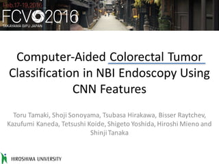
- 12. Experimental setting Training • 907 NBI image patches (Type A: 359, Type B: 461, Type C3: 87) trimmed by medical doctors and endoscopists. • Different sizes: resized to a fixed size (227x227) • Linear SVM (with parameter C by 3-fold CV) • Average accuracy of 10-fold CV Type A: Type B: Type C3: Image patches trimming patch Full size frame
- 13. ���� ����� ������������� ����� ����� ������������� �������������� ����� ���������� ����� ����� ���������� ����� ����� ������������� ����� �������������� 1st layer 2nd layer Visualization by draw_net.py in Caffe Layers and features: an example Figure 2: An illustration of the architecture of our CNN, explicitly showing the delineation of responsibilities between the two GPUs. One GPU runs the layer-parts at the top of the figure while the other runs the layer-parts at the bottom. The GPUs communicate only at certain layers. The network’s input is 150,528-dimensional, and the number of neurons in the network’s remaining layers is given by 253,440–186,624–64,896–64,896–43,264– 4096–4096–1000. neurons in a kernel map). The second convolutional layer takes as input the (response-normalized and pooled) output of the first convolutional layer and filters it with 256 kernels of size 5 ⇥ 5 ⇥ 48. The third, fourth, and fifth convolutional layers are connected to one another without any intervening pooling or normalization layers. The third convolutional layer has 384 kernels of size 3 ⇥ 3 ⇥
- 14. Results for AlexNet ������������� ���� ����� ����� ������������� ���� ����� ������������� ����� ����� ������������� ����� ����� ��� ������������� �������������� �������������� ����� ��� ��� ������������� ���������� ����� ����� ��� ������������� ���������� ����� ����� ������������� ��� ����� ����� ������������� ��� ����� �������������� Figure 2: An illustration of the architecture of our CNN, explicitly showing the delineation of responsibilities between the two GPUs. One GPU runs the layer-parts at the top of the figure while the other runs the layer-parts at the bottom. The GPUs communicate only at certain layers. The network’s input is 150,528-dimensional, and the number of neurons in the network’s remaining layers is given by 253,440–186,624–64,896–64,896–43,264– 4096–4096–1000. neurons in a kernel map). The second convolutional layer takes as input the (response-normalized and pooled) output of the first convolutional layer and filters it with 256 kernels of size 5 ⇥ 5 ⇥ 48. The third, fourth, and fifth convolutional layers are connected to one another without any intervening pooling or normalization layers. The third convolutional layer has 384 kernels of size 3 ⇥ 3 ⇥ 256 connected to the (normalized, pooled) outputs of the second convolutional layer. The fourth convolutional layer has 384 kernels of size 3 ⇥ 3 ⇥ 192 , and the fifth convolutional layer has 256 kernels of size 3 ⇥ 3 ⇥ 192. The fully-connected layers have 4096 neurons each. 4 Reducing Overfitting Our neural network architecture has 60 million parameters. Although the 1000 classes of ILSVRC make each training example impose 10 bits of constraint on the mapping from image to label, this turns out to be insufficient to learn so many parameters without considerable overfitting. Below, we describe the two primary ways in which we combat overfitting. 4.1 Data Augmentation The easiest and most common method to reduce overfitting on image data is to artificially enlarge the dataset using label-preserving transformations (e.g., [25, 4, 5]). We employ two distinct forms of data augmentation, both of which allow transformed images to be produced from the original images with very little computation, so the transformed images do not need to be stored on disk. In our implementation, the transformed images are generated in Python code on the CPU while the GPU is training on the previous batch of images. So these data augmentation schemes are, in effect, computationally free. The first form of data augmentation consists of generating image translations and horizontal reflec- tions. We do this by extracting random 224 ⇥ 224 patches (and their horizontal reflections) from the 256⇥256 images and training our network on these extracted patches4 . This increases the size of our training set by a factor of 2048, though the resulting training examples are, of course, highly inter- dependent. Without this scheme, our network suffers from substantial overfitting, which would have forced us to use much smaller networks. At test time, the network makes a prediction by extracting five 224 ⇥ 224 patches (the four corner patches and the center patch) as well as their horizontal reflections (hence ten patches in all), and averaging the predictions made by the network’s softmax layer on the ten patches. The second form of data augmentation consists of altering the intensities of the RGB channels in training images. Specifically, we perform PCA on the set of RGB pixel values throughout the ImageNet training set. To each training image, we add multiples of the found principal components, 4 This is the reason why the input images in Figure 2 are 224 ⇥ 224 ⇥ 3-dimensional. 5 dimension accuracy
- 15. Results for AlexNet ������������� ���� ����� ����� ������������� ���� ����� ������������� ����� ����� ������������� ����� ����� ��� ������������� �������������� �������������� ����� ��� ��� ������������� ���������� ����� ����� ��� ������������� ���������� ����� ����� ������������� ��� ����� ����� ������������� ��� ����� �������������� Figure 2: An illustration of the architecture of our CNN, explicitly showing the delineation of responsibilities between the two GPUs. One GPU runs the layer-parts at the top of the figure while the other runs the layer-parts at the bottom. The GPUs communicate only at certain layers. The network’s input is 150,528-dimensional, and the number of neurons in the network’s remaining layers is given by 253,440–186,624–64,896–64,896–43,264– 4096–4096–1000. neurons in a kernel map). The second convolutional layer takes as input the (response-normalized and pooled) output of the first convolutional layer and filters it with 256 kernels of size 5 ⇥ 5 ⇥ 48. The third, fourth, and fifth convolutional layers are connected to one another without any intervening pooling or normalization layers. The third convolutional layer has 384 kernels of size 3 ⇥ 3 ⇥ 256 connected to the (normalized, pooled) outputs of the second convolutional layer. The fourth convolutional layer has 384 kernels of size 3 ⇥ 3 ⇥ 192 , and the fifth convolutional layer has 256 kernels of size 3 ⇥ 3 ⇥ 192. The fully-connected layers have 4096 neurons each. 4 Reducing Overfitting Our neural network architecture has 60 million parameters. Although the 1000 classes of ILSVRC make each training example impose 10 bits of constraint on the mapping from image to label, this turns out to be insufficient to learn so many parameters without considerable overfitting. Below, we describe the two primary ways in which we combat overfitting. 4.1 Data Augmentation The easiest and most common method to reduce overfitting on image data is to artificially enlarge the dataset using label-preserving transformations (e.g., [25, 4, 5]). We employ two distinct forms of data augmentation, both of which allow transformed images to be produced from the original images with very little computation, so the transformed images do not need to be stored on disk. In our implementation, the transformed images are generated in Python code on the CPU while the GPU is training on the previous batch of images. So these data augmentation schemes are, in effect, computationally free. The first form of data augmentation consists of generating image translations and horizontal reflec- tions. We do this by extracting random 224 ⇥ 224 patches (and their horizontal reflections) from the 256⇥256 images and training our network on these extracted patches4 . This increases the size of our training set by a factor of 2048, though the resulting training examples are, of course, highly inter- dependent. Without this scheme, our network suffers from substantial overfitting, which would have forced us to use much smaller networks. At test time, the network makes a prediction by extracting five 224 ⇥ 224 patches (the four corner patches and the center patch) as well as their horizontal reflections (hence ten patches in all), and averaging the predictions made by the network’s softmax layer on the ten patches. The second form of data augmentation consists of altering the intensities of the RGB channels in training images. Specifically, we perform PCA on the set of RGB pixel values throughout the ImageNet training set. To each training image, we add multiples of the found principal components, 4 This is the reason why the input images in Figure 2 are 224 ⇥ 224 ⇥ 3-dimensional. 5 pool2: 95.8±2.6% fc6: 95.0±2.9% 43264 4096
- 16. Results for CaffeNet ������������� ���� ����� ����� ������������� ���� ����� ������������� ����� ���������� ����� ����� ��� ������������� �������������� �������������� ����� ��� ��� ������������� ���������� ����� ����� ����� ������������� ��� ������������� ����� ����� ������������� ��� ����� ��� �������������� ����� ����� ������������� Figure 2: An illustration of the architecture of our CNN, explicitly showing the delineation of responsibilities between the two GPUs. One GPU runs the layer-parts at the top of the figure while the other runs the layer-parts at the bottom. The GPUs communicate only at certain layers. The network’s input is 150,528-dimensional, and the number of neurons in the network’s remaining layers is given by 253,440–186,624–64,896–64,896–43,264– 4096–4096–1000. neurons in a kernel map). The second convolutional layer takes as input the (response-normalized and pooled) output of the first convolutional layer and filters it with 256 kernels of size 5 ⇥ 5 ⇥ 48. The third, fourth, and fifth convolutional layers are connected to one another without any intervening pooling or normalization layers. The third convolutional layer has 384 kernels of size 3 ⇥ 3 ⇥ 256 connected to the (normalized, pooled) outputs of the second convolutional layer. The fourth convolutional layer has 384 kernels of size 3 ⇥ 3 ⇥ 192 , and the fifth convolutional layer has 256 kernels of size 3 ⇥ 3 ⇥ 192. The fully-connected layers have 4096 neurons each. 4 Reducing Overfitting Our neural network architecture has 60 million parameters. Although the 1000 classes of ILSVRC make each training example impose 10 bits of constraint on the mapping from image to label, this turns out to be insufficient to learn so many parameters without considerable overfitting. Below, we describe the two primary ways in which we combat overfitting. 4.1 Data Augmentation The easiest and most common method to reduce overfitting on image data is to artificially enlarge the dataset using label-preserving transformations (e.g., [25, 4, 5]). We employ two distinct forms of data augmentation, both of which allow transformed images to be produced from the original images with very little computation, so the transformed images do not need to be stored on disk. In our implementation, the transformed images are generated in Python code on the CPU while the GPU is training on the previous batch of images. So these data augmentation schemes are, in effect, computationally free. The first form of data augmentation consists of generating image translations and horizontal reflec- tions. We do this by extracting random 224 ⇥ 224 patches (and their horizontal reflections) from the 256⇥256 images and training our network on these extracted patches4 . This increases the size of our training set by a factor of 2048, though the resulting training examples are, of course, highly inter- dependent. Without this scheme, our network suffers from substantial overfitting, which would have forced us to use much smaller networks. At test time, the network makes a prediction by extracting five 224 ⇥ 224 patches (the four corner patches and the center patch) as well as their horizontal reflections (hence ten patches in all), and averaging the predictions made by the network’s softmax layer on the ten patches. The second form of data augmentation consists of altering the intensities of the RGB channels in training images. Specifically, we perform PCA on the set of RGB pixel values throughout the ImageNet training set. To each training image, we add multiples of the found principal components, 4 This is the reason why the input images in Figure 2 are 224 ⇥ 224 ⇥ 3-dimensional. 5 pool then normalize conv3: 96.8±2.0% 64896 fc6: 95.8±2.6% 4096
- 17. Figure 2: An illustration of the architecture of our CNN, explicitly showing the delineation of responsibilities between the two GPUs. One GPU runs the layer-parts at the top of the figure while the other runs the layer-parts at the bottom. The GPUs communicate only at certain layers. The network’s input is 150,528-dimensional, and the number of neurons in the network’s remaining layers is given by 253,440–186,624–64,896–64,896–43,264– 4096–4096–1000. neurons in a kernel map). The second convolutional layer takes as input the (response-normalized and pooled) output of the first convolutional layer and filters it with 256 kernels of size 5 ⇥ 5 ⇥ 48. The third, fourth, and fifth convolutional layers are connected to one another without any intervening pooling or normalization layers. The third convolutional layer has 384 kernels of size 3 ⇥ 3 ⇥ 256 connected to the (normalized, pooled) outputs of the second convolutional layer. The fourth convolutional layer has 384 kernels of size 3 ⇥ 3 ⇥ 192 , and the fifth convolutional layer has 256 kernels of size 3 ⇥ 3 ⇥ 192. The fully-connected layers have 4096 neurons each. 4 Reducing Overfitting Our neural network architecture has 60 million parameters. Although the 1000 classes of ILSVRC make each training example impose 10 bits of constraint on the mapping from image to label, this turns out to be insufficient to learn so many parameters without considerable overfitting. Below, we describe the two primary ways in which we combat overfitting. 4.1 Data Augmentation The easiest and most common method to reduce overfitting on image data is to artificially enlarge the dataset using label-preserving transformations (e.g., [25, 4, 5]). We employ two distinct forms of data augmentation, both of which allow transformed images to be produced from the original images with very little computation, so the transformed images do not need to be stored on disk. In our implementation, the transformed images are generated in Python code on the CPU while the GPU is training on the previous batch of images. So these data augmentation schemes are, in effect, computationally free. The first form of data augmentation consists of generating image translations and horizontal reflec- tions. We do this by extracting random 224 ⇥ 224 patches (and their horizontal reflections) from the 256⇥256 images and training our network on these extracted patches4 . This increases the size of our training set by a factor of 2048, though the resulting training examples are, of course, highly inter- dependent. Without this scheme, our network suffers from substantial overfitting, which would have forced us to use much smaller networks. At test time, the network makes a prediction by extracting five 224 ⇥ 224 patches (the four corner patches and the center patch) as well as their horizontal reflections (hence ten patches in all), and averaging the predictions made by the network’s softmax layer on the ten patches. The second form of data augmentation consists of altering the intensities of the RGB channels in training images. Specifically, we perform PCA on the set of RGB pixel values throughout the ImageNet training set. To each training image, we add multiples of the found principal components, 4 This is the reason why the input images in Figure 2 are 224 ⇥ 224 ⇥ 3-dimensional. 5 Results for CaffeNet ������������� ���� ����� ����� ������������� ���� ����� ������������� ����� ���������� ����� ����� ��� ������������� �������������� �������������� ����� ��� ��� ������������� ���������� ����� ����� ����� ������������� ��� ������������� ����� ����� ������������� ��� ����� ��� �������������� ����� ����� ������������� Combinations don’t help
- 20. Results for hand-crafted features BoVW Fisher vector VLAD 97.2±0.3% 32768
- 21. Discussions AlexNet CaffeNet GoogLeNet p First few layers are enough to reach maximum accuracy. p Shallow is enough. p BoVW, FV, VLAD work well.
- 22. Discussions AlexNet CaffeNet GoogLeNet p Pooling layers may work well.
- 23. Discussions AlexNet CaffeNet GoogLeNet p Deeper layers do not help so much. p Full connected layers keep performance while reducing dimension. p Dimensionality reduction (PCA, etc.) may replace it.
- 24. Discussions AlexNet CaffeNet GoogLeNet p Data itself (pixel intensity) is no use. p Probability can be a feature ?! 59.0±4.3% 85.4±4.7% 85.7±4.7% 80.7±2.4%
- 25. Conclusions • Compared off-the-shelf features from three CNN models • Shallow is enough for NBI image classification • A possible architecture is: Dimension reduction (PCA) Classifier (SVM) Shallow CNN with fewer filters
- 27. Results for GoogLeNet: pooling ������������ ����������������������� ������������� �������������������������� ���������������� ������������� ����������������������� ������������� ���������������� ��������������������������� ����������������������� ������������� ����������������������� ���������������� ��������������������������� ����������������������� ���������������� ������������� ��������������� ������������� ��������������� ���������������� ��������������������������� ��������������������� ������������ ���������������� ��������������������������� ��������������� ����������������������� ������������� ����������������������� ����������������� ���������������������� ������������� ���������������� ������������� ���������������� ���������������� ������������� ���������������� ����������������� ���������������������� ������������� ����������������������� ���������������� ������������� ���������������������� ����������������������� ������������� ����������������������� ���������������������� ��������������������������� ������������ ����������������������� ������������� ����������������������� ������������� �������������������������� ���������������� ������������� ������������������� ������������ ����������������������� ������������� ���������������� ������������� ����������������������� ������������� �������������������������� �������� ���������������� ��������������������������� ������������������� �������������� ���������� ������������� ��������� ���������������� ���������������� ������������� ����������������������� ������������������� ���������������� ������������� ����������������������� ������������� ������������������������������������������������� ����������������������� ������������� ���������������� ������������� ���������������� ���������������� ��������������������������� ����������������� ���������������������� ������������� ���������������������� ������������� ���������������������� ���������� �������� ������������� ����������� ��������������������� ���������������������� ��������������� ������������� ���������������� ������������� ���������������� ����������������������� ���������������� ������������� ��������������������� ������������ ��������� ������������� ����������������� ���������������������� ������������� ���������������������� ��������������������������� ����������������������� ���������������� ������������� ���������������� ��������������������������� ������������������� ����������������������� ��������������� ������������� ����������������������� ���������������������� ������������� ���������������������� �������������������������� �������������������������� ����������������� ���������������� �������� ������������������� ���������������������� ������������� ��������������� �������� ������������� ���������������� ���������������� ���������������� ����������������������� ���������������� ������������� ����������������������� ���������������� ������������� ������������������� ��������������������� ����������������������� ������������� ����������������������� ������������� ���������������� ���������� ������������� ���������������� ����������������������� ������������� ����������������������� ���������������� ������������� ���������������� ���������������� ������������� �������������� ����������������������� ����������������������� ������������� ���� ���������������������� ���� ������������ ������������� ���������������� ���������������� �������������������������� ���������� ���������������� ������������� ����������������������� ������������� �������������������������� ����������������������� ���������������� ������������� ���������������� ����������������� ���������������� ������������ ���������������� ������������� ����������������������� ������������� ���������������� ����������� ���������������������� ������������� ���������������������� ����������������������� ������������� ����������������������� ����������������� ���������������� ���������������� ������������������� ���������������������� ���������������� ���������������� �������������������������� ���������������� ������������� ����������������� ���������������� ���������������� ������������� ���������������� ����������������������� ���������������� ������������� ���������������� ������������� ���������������������� ������������� ���������������� ������������� ����������������� ����������������������� ������������� ����������������������� ���������������� ������������� ������������������� ���������������� ������������� ������������������� ��������������������� ���������������� �������������