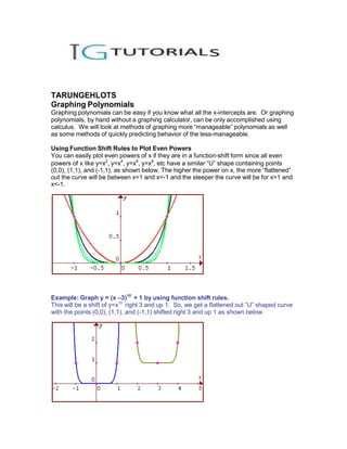
1. TARUNGEHLOTS
Graphing Polynomials
Graphing polynomials can be easy if you know what all the x-intercepts are. Or graphing
polynomials, by hand without a graphing calculator, can be only accomplished using
calculus. We will look at methods of graphing more “manageable” polynomials as well
as some methods of quickly predicting behavior of the less-manageable.
Using Function Shift Rules to Plot Even Powers
You can easily plot even powers of x if they are in a function-shift form since all even
powers of x like y=x2, y=x4, y=x6, y=x8, etc have a similar “U” shape containing points
(0,0), (1,1), and (-1,1), as shown below. The higher the power on x, the more “flattened”
out the curve will be between x=1 and x=-1 and the steeper the curve will be for x>1 and
x<-1.
Example: Graph y = (x –3)10 + 1 by using function shift rules.
This will be a shift of y=x10 right 3 and up 1. So, we get a flattened out “U” shaped curve
with the points (0,0), (1,1), and (-1,1) shifted right 3 and up 1 as shown below.

3. Using Function Shift Rules to Plot Odd Powers
You can easily plot odd powers of x if they are in a function-shift form since all even
powers of x like y=x3, y=x5, y=x7, y=x9, etc have a similar “S” shape containing points
(0,0), (1,1), and (-1,-1), as shown below. The higher the power on x, the more “flattened”
out the curve will be between x=1 and x=-1 and the steeper the curve will be for x>1 and
x<-1, as was the case with the even powers.
Example: Graph y = (x + 2)11 - 1 by using function shift rules.
This will be a shift of y=x11 left 2 and down 1. So, we get a flattened out “S” shaped
curve with the points (0,0), (1,1), and (-1,-1) shifted left 2 and down 1 as shown below.
Leading Term Test For Polynomials
Often, your polynomial does not fit the simple form of the previous two examples, and
function shift rules do not apply. We can still make predictions about the behavior of the
graph by using the Leading Term Test, which in summary, states:
The leading term of a polynomial will predict the behavior of the graph on the far
right side and far left side.

4. Example: Use the Leading Term Test to predict the behavior of the graph of
f(x) = -x5 + 2x + 1.
The leading term is –x5. For positive x-values, this term is negative. So the graph will
fall on the far right. Why does this happen? The leading term has the highest power of
x and thus “dominates” the function in determining what the graph does as x gets larger.
For negative values of x, –x5 is positive. So the graph will rise on the far left. Again,
the leading term has the highest power of x and thus “dominates” the function in
determining what the graph does as x takes on larger negative values.
The leading term test tells us what happens on the far right and far left, and our
conclusions are verified below in the actual graph.
Graphing Polynomials With Known Zeros
If you know the zeros of a polynomial, or they may be determined by factoring, then you
can use the procedure covered back in graphs of functions. The method and example
are given below.
Intercepts Method For Graphing Functions
1. Find and plot all intercepts. To find y-intercepts, let x=0 and solve for y. To find
x-intercepts, let y=0 and solve for x.
2. Plot points on each side of each x-intercept. Find and plot at least one point
between each two x-intercepts and one point on each side of the largest and
smallest x-intercept.
3. Draw a smooth curve through the points from left to right.
Example: Graph f(x) = x3 – x.
First, rewrite as y = x3 – x. Now, find intercepts.
When x = 0, we get y = 03 – 0 = 0. So our y-intercept is (0,0)
When y=0, we get 0 = x3 – x. We solve this equation.
0 = x3 – x Given
0 = x(x2 – 1) Use Distributive Property to factor out x.
0 = x(x + 1)(x – 1) Use Distributive Property to factor x2 – 1.
CONTINUED ON NEXT PAGE

5. x=0 The Zero Product Law allows us to let each factor = 0
x+1=0
x–1=0
x = -1, x = 1, x = 0 Solve each equation using Addition Property of Equality
So the x-intercepts are (-1,0), (1,0), and (0,0)
We plot these points to get
Now, find and plot points on each side of each of these x-intercepts by letting x= -2, x=-
1/2, x=1/2, and x=2. Draw a smooth curve through the points. Note that you could also
use the Leading Term Test to predict that the graph rises to the far right since x3 is
positive for x>0 and falls to the far left since x3 is negative for x<0. The Leading Term
Test would allow us to skip plotting the points (2,6) and (-2,-6).
We get the points
x y
-2 -6
2 6
-1/2 3/8
1/2 -3/8

6. Multiplicity Rules For Polynomial Zeros
The multiplicity of a zero x=c refers to the power N on the factor (x – c)N where (x – c)N is
part of the factorization of the polynomial.
3 2
For example, if f(x) = (x – 2) (x – 5) , then f(x) will have zero x=2 with multiplicity 3 and
zero x = 5 with multiplicity 2. We know x=2 and x=5 are zeros since f(2) = 0 and
f(5) = 0.
If a real zero has even multiplicity, then the graph will “bounce off” the x-intercept
corresponding to the zero. (Remember that x-intercepts occur at real zeros).
If a real zero has odd multiplicity, then the graph will “pass through” the x-intercept
corresponding to the zero. (Remember that x-intercepts occur at real zeros).
2
(x , the graph will (bounce
off) the point (5,0) since x=5 has even multiplicity and the graph will pass through the
point (2,0) since x=2 has odd multiplicity. These conclusions are verified below in the
graph of f(x).
Why Do These Multiplicity Rules Work?
When a factor is raised to an even power, then values above and below the value of the
2
(x ,
the x-value x = 4.9 results in
3 2
f(4.9) = (4.9 – 2) (4.9 – 5) = 2.93 (-.1)2 = 24.389 0.01 = 0.24389
and when x=5.1, we get
3 2
f(5.1) = (5.1 – 2) (5.1 – 5) = 3.13 (.1)2 = 29.791 0.01 = 0.29791
The even power resulted in a positive result each time, so the graph “bounces off”.
When a factor is raised to an odd power, then values above and below the value of the
2
(x , the
x-value x = 2.1 results in
3 2
f(2.1) = (2.1 – 2) (2.1 – 5) = 0.13 (-2.9)2 = 0.001 8.41 = 0.00841
and when x=1.9, we get
3 2
f(1.9) = (1.9 – 2) (1.9 – 5) = (-0.1)3 (-3.1)2 = -0.001 9.61 = -0.00961
The odd power resulted in a negative result at x=1.9 and a positive result at x=2.1.

7. Example: Given f(x) = x3 – x2 – 5x – 3, use the fact that x=3 is a zero to write f(x) in
completely factored form. Then use this form to find all the zeros and then graph. Show
all x-intercepts and make use of the Multiplicity Rules.
Given that x=3 is a zero, this means that (x – 3) is a factor. So if we divide f(x) by
(x – 3), we are able to write f(x) as a product of (x-3) and this result.
We can divide f(x) using synthetic division. Synthetic division results in a zero remainder
(as it should be!)
So this means f(x) = (x – 3)(x2 + 2x + 1). We can factor this some more to get
f(x) = (x – 3)(x +1)(x + 1) or
f(x) = (x – 3)(x+1)2
The factor (x-3) is raised to the 1st power so it has odd multiplicity 1.
The factor (x+1) is raised to the 2nd power so is has even multiplicity 2.
So, with this information, we know that :
ƒ The graph has x-intercepts (3,0) and (-1,0).
ƒ The graph “bounces off” the point (-1,0) and passes through the point (3,0).
ƒ Also, the Leading Term test predicts that the graph rises up to the right since
leading term x3 is positive for x>0 and falls to the left since leading term x3 is
negative for x<0.
Putting all this together, we conclude that the graph bounces off (-1,0) from below since it
is negative on the far left. Also, we conclude that it must rise up again and pass through
(3,0) in order to rise up on the far right. Finding a few more points like (0,-3) and (1,-8)
also help to give us a little better picture of the graph. The graph is shown below.
Students often ask, “How low will the graph go in between the x-intercepts? Is there
something like the vertex (of a parabola) that we can calculate for higher order
polynomials?” The answer is: Yes, you can find this “low point” exactly, but you need to
use calculus in order to do so.