Appendex f

October 22, 2004 14:05 k34-appf Sheet number 1 Page number 47 cyan magenta yellow black
PAGE PROOFS
A47
a p p e n d i x f
COORDINATE PLANES, LINES,
AND LINEAR FUNCTIONS
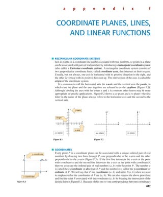
RECTANGULAR COORDINATE SYSTEMS
Just as points on a coordinate line can be associated with real numbers, so points in a plane
can be associated with pairs of real numbers by introducing a rectangular coordinate system
(also called a Cartesian coordinate system). A rectangular coordinate system consists of
two perpendicular coordinate lines, called coordinate axes, that intersect at their origins.
Usually, but not always, one axis is horizontal with its positive direction to the right, and
the other is vertical with its positive direction up. The intersection of the axes is called the
origin of the coordinate system.
It is common to call the horizontal axis the x-axis and the vertical axis the y-axis, in
which case the plane and the axes together are referred to as the xy-plane (Figure F.1).
Although labeling the axes with the letters x and y is common, other letters may be more
appropriate in specific applications. Figure F.2 shows a uv-plane and a ts-plane—the first
letter in the name of the plane always refers to the horizontal axis and the second to the
vertical axis.
xy-plane
x
y
-4 -3 -2 -1 1 2 3 4
-4
-3
-2
-1
0
1
2
3
4
y-axis
x-axis
Origin
Figure F.1
uv-plane ts-plane
u
v
t
s
Figure F.2
COORDINATES
Every point P in a coordinate plane can be associated with a unique ordered pair of real
numbers by drawing two lines through P, one perpendicular to the x-axis and the other
perpendicular to the y-axis (Figure F.3). If the first line intersects the x-axis at the point
with coordinate a and the second line intersects the y-axis at the point with coordinate b,
then we associate the ordered pair of real numbers (a, b) with the point P. The number a
is called the x-coordinate or abscissa of P and the number b is called the y-coordinate or
ordinate of P. We will say that P has coordinates (a, b) and write P(a, b) when we want
to emphasize that the coordinates of P are (a, b). We can also reverse the above procedure
and find the point P associated with the coordinates (a, b) by locating the intersection of the
dashed lines in Figure F.3. Because of this one-to-one correspondence between coordinates
y-coordinate
x-coordinate
b P(a, b)
a
Figure F.3

PAGE PROOFS
A48 Appendix F: Coordinate Planes, Lines, and Linear Functions
and points, we will sometimes blur the distinction between points and ordered pairs of
numbers by talking about the point (a, b).
Recall that the symbol (a, b) also denotes the open interval between a and b; the appropriate
interpretation will usually be clear from the context.
Inarectangularcoordinatesystemthecoordinateaxesdividetherestoftheplaneintofour
regions called quadrants. These are numbered counterclockwise with roman numerals as
shown in Figure F.4. As indicated in that figure, it is easy to determine the quadrant in which
a given point lies from the signs of its coordinates: a point with two positive coordinates
(+, +) lies in Quadrant I, a point with a negative x-coordinate and a positive y-coordinate
(−, +) lies in Quadrant II, and so forth. Points with a zero x-coordinate lie on the y-axis
and points with a zero y-coordinate lie on the x-axis.
x
y
Quadrant
II
(–, +)
Quadrant
I
(+, +)
Quadrant
III
(–, –)
Quadrant
IV
(+, –)
Figure F.4
To plot a point P(a, b) means to locate the point with coordinates (a, b) in a coordinate
plane. For example, in Figure F.5 we have plotted the points
P(2, 5), Q(−4, 3), R(−5, −2), and S(4, −3)
Observe how the signs of the coordinates identify the quadrants in which the points lie.
-7 -6 -5 -4 -3 -2 -1 1 2 3 4 5 6 7
-5
-4
-3
-2
-1
1
2
3
4
5
6
x
y
P(2, 5)
S(4, –3)
Q(–4, 3)
R(–5, –2)
Figure F.5
GRAPHS
The correspondence between points in a plane and ordered pairs of real numbers makes it
possible to visualize algebraic equations as geometric curves, and, conversely, to represent
geometric curves by algebraic equations. To understand how this is done, suppose that we
have an xy-coordinate system and an equation involving two variables x and y, say
6x − 4y = 10, y =
√
x, x = y3
+ 1, or x2
+ y2
= 1
We define a solution of such an equation to be any ordered pair of real numbers (a, b)
whose coordinates satisfy the equation when we substitute x = a and y = b. For example,
the ordered pair (3, 2) is a solution of the equation 6x − 4y = 10, since the equation is
satisfied by x = 3 and y = 2 (verify). However, the ordered pair (2, 0) is not a solution of
this equation, since the equation is not satisfied by x = 2 and y = 0 (verify).
The following definition makes the association between equations in x and y and curves
in the xy-plane.

PAGE PROOFS
Appendix F: Coordinate Planes, Lines, and Linear Functions A49
F.1 definition. The set of all solutions of an equation in x and y is called the solu-
tion set of the equation, and the set of all points in the xy-plane whose coordinates are
members of the solution set is called the graph of the equation.
One of the main themes in calculus is to identify the exact shape of a graph. Point
plotting is one approach to obtaining a graph, but this method has limitations, as discussed
in the following example.
Example 1 Use point plotting to sketch the graph of y = x2
. Discuss the limitations
of this method.
Solution. The solution set of the equation has infinitely many members, since we can
substitute an arbitrary value for x into the right side of y = x2
and compute the associated
y to obtain a point (x, y) in the solution set. The fact that the solution set has infinitely
many members means that we cannot obtain the entire graph of y = x2
by point plotting.
However, we can obtain an approximation to the graph by plotting some sample members
of the solution set and connecting them with a smooth curve, as in Figure F.6. The problem
with this method is that we cannot be sure how the graph behaves between the plotted
points. For example, the curves in Figure F.7 also pass through the plotted points and hence
are legitimate candidates for the graph in the absence of additional information. Moreover,
even if we use a graphing calculator or a computer program to generate the graph, as in
Figure F.8, we have the same problem because graphing technology uses point-plotting
algorithms to generate graphs. Indeed, in Section 1.2 of the text we see examples where
graphing technology can be fooled into producing grossly inaccurate graphs.
y = x2
x
0
1
2
3
–1
–2
–3
0
1
4
9
1
4
9
(0, 0)
(1, 1)
(2, 4)
(3, 9)
(–1, 1)
(–2, 4)
(–3, 9)
y = x2 (x, y)
-3 -2 -1 1 2 3
1
2
3
4
5
6
7
8
9
x
y
Figure F.6
-3 -2 -1 1 2 3
1
2
3
4
5
6
7
8
9
x
y
-3 -2 -1 1 2 3
1
2
3
4
5
6
7
8
9
x
y
Figure F.7
[–4, 4] × [0, 10]
xScl = 1, yScl = 2
y = x2
Figure F.8
In spite of its limitations, point plotting by hand or with the help of graphing technology
can be useful, so here are two more examples.
Example 2 Sketch the graph of y =
√
x.
Solution. If x < 0, then
√
x is an imaginary number. Thus, we can only plot points for
which x ≥ 0, since points in the xy-plane have real coordinates. Figure F.9 shows the graph
obtained by point plotting and a graph obtained with a graphing calculator.

PAGE PROOFS
1 2 3 4
1
2
3
x
y
x
0
1
2
3
4
y = √x (x, y)
y = √x0
1
√2
√3
2
(0, 0)
(1, 1)
(2, √2) ≈ (2, 1.4)
(3, √3) ≈ (3, 1.7)
(4, 2)
[0, 5] × [0, 4]
xScl = 1, yScl = 1
y = √x
Figure F.9
Example 3 Sketch the graph of y2
− 2y − x = 0.
Solution. To calculate coordinates of points on the graph of an equation in x and y, it is
desirable to have y expressed in terms of x or x in terms of y. In this case it is easier to
express x in terms of y, so we rewrite the equation as
x = y2
− 2y
Members of the solution set can be obtained from this equation by substituting arbitrary
values for y in the right side and computing the associated values of x (Figure F.10).
x = y2
– 2y
y
–2
–1
0
1
2
3
4
8
3
0
–1
0
3
8
(8, –2)
(3, –1)
(0, 0)
(–1, 1)
(0, 2)
(3, 3)
(8, 4)
x = y2 – 2y (x, y)
-1 8
-2
4
x
y
Figure F.10
Most graphing calculators and computer graphing programs require that y be expressed in terms
of x to generate a graph in the xy-plane. In Section 1.8 we discuss a method for circumventing
this restriction.
Example 4 Sketch the graph of y = 1/x.
Solution. Because 1/x is undeﬁned at x = 0, we can only plot points for which x = 0.
This forces a break, called a discontinuity, in the graph at x = 0 (Figure F.11).
INTERCEPTS
Points where a graph intersects the coordinate axes are of special interest in many problems.
As illustrated in Figure F.12, intersections of a graph with the x-axis have the form (a, 0)
and intersections with the y-axis have the form (0, b). The number a is called an x-intercept
of the graph and the number b a y-intercept.

PAGE PROOFS
x
1
2
3
–1
–2
–3
3
2
1
–3
–2
–1
y = 1/x
y = 1/x
(x, y)
2
1
3
1
2
1
3
1
–
–
2
1
3
1
–
–
3
1
2
1
–
–
3
1
2
1
–
–
3
1
2
1
3
1
2
1
2
1
3
1
( , 3)
( , 2)
(1, 1)
(2, )
(3, )
( , –3)
( , –2)
(–1, –1)
(–2, )
(–3, )
1 2 3 4
1
2
3
4
x
y
Figure F.11
Example 5 Find all intercepts of
(a) 3x + 2y = 6 (b) x = y2
− 2y (c) y = 1/x
x
y
(0, b)
(a, 0)
y-intercept is b
x-intercept is a
Figure F.12
Solution (a). To find the x-intercepts we set y = 0 and solve for x:
3x = 6 or x = 2
To find the y-intercepts we set x = 0 and solve for y:
2y = 6 or y = 3
As we will see later, the graph of 3x + 2y = 6 is the line shown in Figure F.13.
2
3
x
y
3x + 2y = 6
Figure F.13
Solution (b). To find the x-intercepts, set y = 0 and solve for x:
x = 0
Thus, x = 0 is the only x-intercept. To find the y-intercepts, set x = 0 and solve for y:
y2
− 2y = 0
y(y − 2) = 0
So the y-intercepts are y = 0 and y = 2. The graph is shown in Figure F.10.
Solution (c). To find the x-intercepts, set y = 0:
1
x
= 0
This equation has no solutions (why?), so there are no x-intercepts. To find y-intercepts we
would set x = 0 and solve for y. But, substituting x = 0 leads to a division by zero, which
is not allowed, so there are no y-intercepts either. The graph of the equation is shown in
Figure F.11.
SLOPE
To obtain equations of lines we will first need to discuss the concept of slope, which is a
numerical measure of the “steepness” of a line.

PAGE PROOFS
Consider a particle moving left to right along a nonvertical line from a point P1(x1, y1)
to a point P2(x2, y2). As shown in Figure F.14, the particle moves y2 − y1 units in the y-
direction as it travels x2 − x1 units in the positive x-direction. The vertical change y2 − y1
is called the rise, and the horizontal change x2 − x1 the run. The ratio of the rise over
the run can be used to measure the steepness of the line, which leads us to the following
definition.
x
y
P1(x1, y1)
P2(x2, y2)
(Run)
(Rise)
x2 – x1
y2–y1
Figure F.14
F.2 definition. If P1(x1, y1) and P2(x2, y2) are points on a nonvertical line, then
the slope m of the line is defined by
m =
rise
run
=
y2 − y1
x2 − x1
(1)
Observe that this definition does not apply to vertical lines. For such lines we have x2 = x1 (a zero
run), which means that the formula for m involves a division by zero. For this reason, the slope of
a vertical line is undefined, which is sometimes described informally by stating that a vertical line
has infinite slope.
When calculating the slope of a nonvertical line from Formula (1), it does not matter
which two points on the line you use for the calculation, as long as they are distinct. This
can be proved using Figure F.15 and similar triangles to show that
P1′(x1′, y1′)
P2′(x2′, y2′)
P2(x2, y2)
y2–y1
y2′–y1′
x2′ – x1′
x2 – x1
P1(x1, y1)
x
y
Figure F.15
m =
y2 − y1
x2 − x1
=
y2 − y1
x2 − x1
Moreover, once you choose two points to use for the calculation, it does not matter which
one you call P1 and which one you call P2 because reversing the points reverses the sign
of both the numerator and denominator of (1) and hence has no effect on the ratio.
Example 6 In each part find the slope of the line through
(a) the points (6, 2) and (9, 8)
(b) the points (2, 9) and (4, 3)
(c) the points (−2, 7) and (5, 7).
Solution.
(a) m =
8 − 2
9 − 6
=
6
3
= 2 (b) m =
3 − 9
4 − 2
=
−6
2
= −3 (c) m =
7 − 7
5 − (−2)
= 0
Example 7 Figure F.16 shows the three lines determined by the points in Example 6
and explains the significance of their slopes.
As illustrated in this example, the slope of a line can be positive, negative, or zero. A
positive slope means that the line is inclined upward to the right, a negative slope means that
the line is inclined downward to the right, and a zero slope means that the line is horizontal.
An undefined slope means that the line is vertical. Figure F.17 shows various lines through
the origin with their slopes.

PAGE PROOFS
P2(9, 8)
P1(6, 2)
P1(2, 9)
P2(4, 3)
3
6
Traveling left to right, a point on the
line rises two units for each unit it
moves in the positive x-direction.
m = 0
Traveling left to right, a point on
the line neither rises nor falls.
6
2
Traveling left to right, a point on the
line falls three units for each unit it
moves in the positive x-direction.
m = 2 m = –3
(5, 7)(–2, 7)
x
y
x
y
x
y
Figure F.16
PARALLEL AND PERPENDICULAR LINES
The following theorem shows how slopes can be used to tell whether two lines are parallel
or perpendicular.
F.3 theorem.
(a) Two nonvertical lines with slopes m1 and m2 are parallel if and only if they have
the same slope, that is,
m1 = m2
(b) Two nonvertical lines with slopes m1 and m2 are perpendicular if and only if the
product of their slopes is −1, that is,
m1m2 = −1
This relationship can also be expressed as m1 = −1/m2 or m2 = −1/m1, which
statesthatnonverticallinesareperpendicularifandonlyiftheirslopesarenegative
reciprocals of one another.
Negative
slope
m = 3
m = –3
m = 2
m = 1
m = –1
m = –2
m = 0
Positiv
e
slope
1
2
m =
1
2
m = –
Figure F.17 A complete proof of this theorem is a little tedious, but it is not hard to motivate the results
informally. Let us start with part (a).
Suppose that L1 and L2 are nonvertical parallel lines with slopes m1 and m2, respectively.
If the lines are parallel to the x-axis, then m1 = m2 = 0, and we are done. If they are not
parallel to the x-axis, then both lines intersect the x-axis; and for simplicity assume that
they are oriented as in Figure F.18a. On each line choose the point whose run relative to
the point of intersection with the x-axis is 1. On line L1 the corresponding rise will be m1
and on L2 it will be m2. However, because the lines are parallel, the shaded triangles in the
ﬁgure must be congruent (verify), so m1 = m2. Conversely, the condition m1 = m2 can be
used to show that the shaded triangles are congruent, from which it follows that the lines
make the same angle with the x-axis and hence are parallel (verify).
Now suppose that L1 and L2 are nonvertical perpendicular lines with slopes m1 and m2,
respectively; and for simplicity assume that they are oriented as in Figure F.18b. On line
L1 choose the point whose run relative to the point of intersection of the lines is 1, in which
case the corresponding rise will be m1; and on line L2 choose the point whose rise relative
to the point of intersection is −1, in which case the corresponding run will be −1/m2.
Because the lines are perpendicular, the shaded triangles in the ﬁgure must be congruent

PAGE PROOFS
Run = 1
Rise = m1
Run = 1
Rise = m2
L1 L2
x
(a)
Run = 1Run = –1/m2
Rise = m1
Rise = –1
L1
L2
(b)
Figure F.18
(verify), and hence the ratios of corresponding sides of the triangles must be equal. Taking
into account that for line L2 the vertical side of the triangle has length 1 and the horizontal
side has length −1/m2 (since m2 is negative), the congruence of the triangles implies that
m1/1 = (−1/m2)/1 or m1m2 = −1. Conversely, the condition m1 = −1/m2 can be used
to show that the shaded triangles are congruent, from which it can be deduced that the lines
are perpendicular (verify).
Example 8 Use slopes to show that the points A(1, 3), B(3, 7), and C(7, 5) are
vertices of a right triangle.
Solution. We will show that the line through A and B is perpendicular to the line through
B and C. The slopes of these lines are
m1 =
7 − 3
3 − 1
= 2 and m2 =
5 − 7
7 − 3
= −
1
2
Slope of the line
through A and B
Slope of the line
through B and C
Since m1m2 = −1, the line through A and B is perpendicular to the line through B and C;
thus, ABC is a right triangle (Figure F.19).
x
y
A(1, 3)
C(7, 5)
B(3, 7)
Figure F.19
LINES PARALLEL TO THE COORDINATE AXES
We now turn to the problem of ﬁnding equations of lines that satisfy speciﬁed conditions.
The simplest cases are lines parallel to the coordinate axes. A line parallel to the y-axis
intersects the x-axis at some point (a, 0). This line consists precisely of those points whose
x-coordinates equal a (Figure F.20). Similarly, a line parallel to the x-axis intersects the
y-axis at some point (0, b). This line consists precisely of those points whose y-coordinates
equal b (Figure F.20). Thus, we have the following theorem.
F.4 theorem. The vertical line through (a, 0) and the horizontal line through (0, b)
are represented, respectively, by the equations
x = a and y = b
(a, 0)
(0, b) L2
L1
Every point on L1 has an
x-coordinate of a and
every point on L2 has a
y-coordinate of b.
x
y
Figure F.20
Example 9 The graph of x = −5 is the vertical line through (−5, 0), and the graph
of y = 7 is the horizontal line through (0, 7) (Figure F.21).

PAGE PROOFS
(–5, 0)
x = –5
y = 7
x
y
(0, 7)
x
y
Figure F.21
LINES DETERMINED BY POINT AND SLOPE
There are infinitely many lines that pass through any given point in the plane. However,
if we specify the slope of the line in addition to a point on it, then the point and the slope
together determine a unique line (Figure F.22).
Let us now consider how to find an equation of a nonvertical line L that passes through
a point P1(x1, y1) and has slope m. If P(x, y) is any point on L, different from P1, then
the slope m can be obtained from the points P(x, y) and P1(x1, y1); this gives
m =
y − y1
x − x1
which can be rewritten as y − y1 = m(x − x1) (2)
With the possible exception of (x1, y1), we have shown that every point on L satisfies (2).
But x = x1, y = y1 satisfies (2), so that all points on L satisfy (2). We leave it as an exercise
to show that every point satisfying (2) lies on L.
m
x
y
P
There is a unique line
through P with slope m.
Figure F.22
In summary, we have the following theorem.
F.5 theorem. The line passing through P1(x1, y1) and having slope m is given by
the equation
y − y1 = m(x − x1) (3)
This is called the point-slope form of the line.
Example 10 Find the point-slope form of the line through (4, −3) with slope 5.
Solution. Substituting the values x1 = 4, y1 = −3, and m = 5 in (3) yields the point-
slope form y + 3 = 5(x − 4).
LINES DETERMINED BY SLOPE AND y-INTERCEPT
A nonvertical line crosses the y-axis at some point (0, b). If we use this point in the
point-slope form of its equation, we obtain
y − b = m(x − 0)
which we can rewrite as y = mx + b. To summarize:
When the equation of a line is written
as in (4), the slope is the coefficient of x
and the y-intercept is the constant term
(Figure F.23).
y = mx + b
Slope y-intercept
Figure F.23
F.6 theorem. The line with y-intercept b and slope m is given by the equation
y = mx + b (4)
This is called the slope-intercept form of the line.

PAGE PROOFS
Example 11
y = 3x + 7
y = –x +
y = x
y = √2x – 8
y = 2
equation slope y-intercept
b = 7
b =
b = 0
b = –8
b = 2
1
2
1
2
m = 3
m = –1
m = 1
m = √2
m = 0
Example 12 Find the slope-intercept form of the equation of the line that satisfies the
stated conditions:
(a) slope is −9; crosses the y-axis at (0, −4)
(b) slope is 1; passes through the origin
(c) passes through (5, −1); perpendicular to y = 3x + 4
(d) passes through (3, 4) and (2, −5).
Solution (a). From the given conditions we have m = −9 and b = −4, so (4) yields
y = −9x − 4.
Solution (b). From the given conditions m = 1 and the line passes through (0, 0), so
b = 0. Thus, it follows from (4) that y = x + 0 or y = x.
Solution (c). The given line has slope 3, so the line to be determined will have slope
m = −1
3
. Substituting this slope and the given point in the point-slope form (3) and then
simplifying yields
y − (−1) = −1
3
(x − 5)
y = −1
3
x + 2
3
Solution (d). We will first find the point-slope form, then solve for y in terms of x to
obtain the slope-intercept form. From the given points the slope of the line is
m =
−5 − 4
2 − 3
= 9
We can use either of the given points for (x1, y1) in (3). We will use (3, 4). This yields the
point-slope form
y − 4 = 9(x − 3)
Solving for y in terms of x yields the slope-intercept form
y = 9x − 23
We leave it for the reader to show that the same equation results if (2, −5) rather than (3, 4)
is used for (x1, y1) in (3).
THE GENERAL EQUATION OF A LINE
An equation that is expressible in the form
Ax + By + C = 0 (5)
where A, B, and C are constants and A and B are not both zero, is called a first-degree
equation in x and y. For example,
4x + 6y − 5 = 0

PAGE PROOFS
is a first-degree equation in x and y since it has form (5) with
A = 4, B = 6, C = −5
In fact, all the equations of lines studied in this section are first-degree equations in x and y.
The following theorem states that the first-degree equations in x and y are precisely the
equations whose graphs in the xy-plane are straight lines.
F.7 theorem. Every first-degree equation in x and y has a straight line as its graph
and, conversely, every straight line can be represented by a first-degree equation in x
and y.
Because of this theorem, (5) is sometimes called the general equation of a line or a
linear equation in x and y.
Example 13 Graph the equation 3x − 4y + 12 = 0.
Solution. Since this is a linear equation in x and y, its graph is a straight line. Thus, to
sketch the graph we need only plot any two points on the graph and draw the line through
them. It is particularly convenient to plot the points where the line crosses the coordinate
axes. These points are (0, 3) and (−4, 0) (verify), so the graph is the line in Figure F.24.
x
y
(0, 3)
(–4, 0)
3x – 4y + 12 = 0
Figure F.24
Example 14 Find the slope of the line in Example 13.
Solution. Solving the equation for y yields
y = 3
4
x + 3
which is the slope-intercept form of the line. Thus, the slope is m = 3
4
.
LINEAR FUNCTIONS
When x and y are related by Equation (4) then we say that y is a linear function of x.
Linear functions arise in a variety of practial problems. Here is a typical example.
Example 15 A university parking lot charges $3.00 per day but offers a $40.00
monthly sticker with which the student pays only $0.25 per day.
(a) Find equations for the cost C of parking for x days per month under both payment
methods, and graph the equations for 0 ≤ x ≤ 30. (Treat C as a continuous function
of x, even though x only assumes integer values.)
(b) Find the value of x for which the graphs intersect, and discuss the significance of this
value.
Solution (a). The cost in dollars of parking for x days at $3.00 per day is C = 3x, and
the cost for the $40.00 sticker plus x days at $0.25 per day is C = 40 + 0.25x (Figure F.25).
5 10 15 20 25 30
10
20
30
40
50
60
70
80
90
100
x
C
Costindollars
C = 3x
C = 40 + 0.25x
Number of parking days
Figure F.25
Solution (b). The graphs intersect at the point where
3x = 40 + 0.25x
which is x = 40/2.75 ≈ 14.5. This value of x is not an option for the student, since x
must be an integer. However, it is the dividing point at which the monthly sticker method

PAGE PROOFS
becomes less expensive than the daily payment method; that is, for x ≥ 15 it is cheaper to
buy the monthly sticker and for x ≤ 14 it is cheaper to pay the daily rate.
DIRECT PROPORTION
A variable y is said to be directly proportional to a variable x if there is a positive constant
k, called the constant of proportionality, such that
y = kx (6)
The graph of this equation is a line through the origin whose slope k is the constant of
proportionality. Thus, linear functions are appropriate in physical problems where one
variable is directly proportional to another.
Hooke’s law
∗
in physics provides a nice example of direct proportion. It follows from
this law that if a weight of x units is suspended from a spring, then the spring will be
stretched by an amount y that is directly proportional to x, that is, y = kx (Figure F.26).
The constant k depends on the stiffness of the spring: the stiffer the spring, the smaller the
value of k (why?).
y
x
y is directly proportional to x.
Figure F.26
Example 16 Figure F.27 shows an old-fashioned spring scale that is calibrated in
pounds.
(a) Given that the pound scale marks are 0.5 in apart, ﬁnd an equation that expresses the
length y that the spring is stretched (in inches) in terms of the suspended weight x (in
pounds).
(b) Graph the equation obtained in part (a).
Figure F.27
0 2 4 6 8 10 12
1
2
3
4
5
6
y = 0.5x
Weight x (lb)
Lengthstretchedy(in)
Solution (a). It follows from Hooke’s law that y is related to x by an equation of the
form y = kx. To ﬁnd k we rewrite this equation as k = y/x and use the fact that a weight
of x = 1 lb stretches the spring y = 0.5 in. Thus,
k =
y
x
=
0.5
1
= 0.5 and hence y = 0.5x
Solution (b). The graph of the equation y = 0.5x is shown in Figure F.27.
∗
Hooke’s law, named for the English physicist Robert Hooke (1635–1703), applies only for small displacements
that do not stretch the spring to the point of permanently distorting it.

PAGE PROOFS
EXERCISE SET F
1. Draw the rectangle, three of whose vertices are (6, 1),
(−4, 1), and (6, 7), and find the coordinates of the fourth
vertex.
2. Draw the triangle whose vertices are (−3, 2), (5, 2), and
(4, 3), and find its area.
3–4 Draw a rectangular coordinate system and sketch the
set of points whose coordinates (x, y) satisfy the given con-
ditions.
3. (a) x = 2 (b) y = −3 (c) x ≥ 0
(d) y = x (e) y ≥ x (f ) |x| ≥ 1
4. (a) x = 0 (b) y = 0
(c) y < 0 (d) x ≥ 1 and y ≤ 2
(e) x = 3 (f ) |x| = 5
5–12 Sketch the graph of the equation. (Acalculating utility
will be helpful in some of these problems.)
5. y = 4 − x2
6. y = 1 + x2
7. y =
√
x − 4 8. y = −
√
x + 1
9. x2
− x + y = 0 10. x = y3
− y2
11. x2
y = 2 12. xy = −1
13. Find the slope of the line through
(a) (−1, 2) and (3, 4) (b) (5, 3) and (7, 1)
(c) (4,
√
2) and (−3,
√
2 ) (d) (−2, −6) and (−2, 12).
14. Find the slopes of the sides of the triangle with vertices
(−1, 2), (6, 5), and (2, 7).
15. Use slopes to determine whether the given points lie on the
same line.
(a) (1, 1), (−2, −5), and (0, −1)
(b) (−2, 4), (0, 2), and (1, 5)
16. Draw the line through (4, 2) with slope
(a) m = 3 (b) m = −2 (c) m = −3
4
.
17. Draw the line through (−1, −2) with slope
(a) m = 3
5
(b) m = −1 (c) m =
√
2.
18. An equilateral triangle has one vertex at the origin, another
on the x-axis, and the third in the first quadrant. Find the
slopes of its sides.
19. List the lines in the accompanying figure in the order of
increasing slope.
x
y
III
x
y
IV
x
y
II
x
y
I
Figure Ex-19
20. List the lines in the accompanying figure in the order of
increasing slope.
x
y
III
x
y
IV
x
y
II
x
y
I
Figure Ex-20
21. A particle, initially at (1, 2), moves along a line of slope
m = 3 to a new position (x, y).
(a) Find y if x = 5. (b) Find x if y = −2.
22. A particle, initially at (7, 5), moves along a line of slope
m = −2 to a new position (x, y).
(a) Find y if x = 9. (b) Find x if y = 12.
23. Let the point (3, k) lie on the line of slope m = 5 through
(−2, 4); find k.
24. Given that the point (k, 4) is on the line through (1, 5) and
(2, −3), find k.
25. Find x if the slope of the line through (1, 2) and (x, 0) is the
negative of the slope of the line through (4, 5) and (x, 0).
26. Find x and y if the line through (0, 0) and (x, y) has slope
1
2
, and the line through (x, y) and (7, 5) has slope 2.
27. Use slopes to show that (3, −1), (6, 4), (−3, 2), and
(−6, −3) are vertices of a parallelogram.
28. Use slopes to show that (3, 1), (6, 3), and (2, 9) are vertices
of a right triangle.
29. Graph the equations
(a) 2x + 5y = 15 (b) x = 3
(c) y = −2 (d) y = 2x − 7.
(a)
x
3
−
y
4
= 1 (b) x = −8
(c) y = 0 (d) x = 3y + 2.
(a) y = 2x − 1 (b) y = 3
(c) y = −2x.
(a) y = 2 − 3x (b) y = 1
4
x
(c) y = −
√
3.
33. Find the slope and y-intercept of
(a) y = 3x + 2 (b) y = 3 − 1
4
x
(c) 3x + 5y = 8 (d) y = 1
(e)
x
a
+
y
b
= 1.
34. Find the slope and y-intercept of
(a) y = −4x + 2 (b) x = 3y + 2
(c)
x
2
+
y
3
= 1 (d) y − 3 = 0
(e) a0x + a1y = 0 (a1 = 0).
35–36 Use the graph to find the equation of the line in slope-
intercept form.

PAGE PROOFS
35.
1
x
y
x
y
1
(a) (b)
Figure Ex-35
36.
1
x
y
1
x
y
(a) (b)
Figure Ex-36
37–48 Find the slope-intercept form of the line satisfying
the given conditions.
37. Slope = −2, y-intercept = 4.
38. m = 5, b = −3.
39. The line is parallel to y = 4x − 2 and its y-intercept is 7.
40. The line is parallel to 3x + 2y = 5 and passes through
(−1, 2).
41. The line is perpendicular to y = 5x + 9 and its y-intercept
is 6.
42. The line is perpendicular to x − 4y = 7 and passes through
(3, −4).
43. The line passes through (2, 4) and (1, −7).
44. The line passes through (−3, 6) and (−2, 1).
45. The y-intercept is 2 and the x-intercept is −4.
46. The y-intercept is b and the x-intercept is a.
47. The line is perpendicular to the y-axis and passes through
(−4, 1).
48. The line is parallel to y = −5 and passes through (−1, −8).
49. In each part, classify the lines as parallel, perpendicular, or
neither.
(a) y = 4x − 7 and y = 4x + 9
(b) y = 2x − 3 and y = 7 − 1
2
x
(c) 5x − 3y + 6 = 0 and 10x − 6y + 7 = 0
(d) Ax + By + C = 0 and Bx − Ay + D = 0
(e) y − 2 = 4(x − 3) and y − 7 = 1
4
(x − 3)
50. In each part, classify the lines as parallel, perpendicular, or
neither.
(a) y = −5x + 1 and y = 3 − 5x
(b) y − 1 = 2(x − 3) and y − 4 = −1
2
(x + 7)
(c) 4x + 5y + 7 = 0 and 5x − 4y + 9 = 0
(d) Ax + By + C = 0 and Ax + By + D = 0
(e) y = 1
2
x and x = 1
2
y
51. For what value of k will the line 3x + ky = 4
(a) have slope 2
(b) have y-intercept 5
(c) pass through the point (−2, 4)
(d) be parallel to the line 2x − 5y = 1
(e) be perpendicular to the line 4x + 3y = 2?
52. Sketch the graph of y2
= 3x and explain how this graph is
related to the graphs of y =
√
3x and y = −
√
3x.
53. Sketch the graph of (x − y)(x + y) = 0 and explain how it
is related to the graphs of x − y = 0 and x + y = 0.
54. Graph F = 9
5
C + 32 in a CF-coordinate system.
55. Graph u = 3v2
in a uv-coordinate system.
56. Graph Y = 4X + 5 in a YX -coordinate system.
57. Apoint moves in the xy-plane in such a way that at any time
t its coordinates are given by x = 5t + 2 and y = t − 3. By
expressing y in terms of x, show that the point moves along
a straight line.
58. Apoint moves in the xy-plane in such a way that at any time
t its coordinates are given by x = 1 + 3t2
and y = 2 − t2
.
By expressing y in terms of x, show that the point moves
along a straight-line path and specify the values of x for
which the equation is valid.
59. Find the area of the triangle formed by the coordinate axes
and the line through (1, 4) and (2, 1).
60. Draw the graph of 4x2
− 9y2
= 0.
61. A spring with a natural length of 15 in stretches to a length
of 20 in when a 45-lb object is suspended from it.
(a) Use Hooke’s law to ﬁnd an equation that expresses the
amount y by which the spring is stretched (in inches) in
terms of the suspended weight x (in pounds).
(c) Find the length of the spring when a 100-lb object is
suspended from it.
(d) What is the largest weight that can be suspended from
the spring if the spring cannot be stretched to more than
twice its natural length?
62. The spring in a heavy-duty shock absorber has a natural
length of 3 ft and is compressed 0.2 ft by a load of 1 ton. An
additional load of 5 tons compresses the spring an additional
1 ft.
(a) Assuming that Hooke’s law applies to compression as
well as extension, ﬁnd an equation that expresses the
length y that the spring is compressed from its natural
length (in feet) in terms of the load x (in tons).
(c) Find the amount that the spring is compressed from its
natural length by a load of 3 tons.
(d) Find the maximum load that can be applied if safety
regulations prohibit compressing the spring to less than
half its natural length.

PAGE PROOFS
63–64 Confirm that a linear function is appropriate for the
relationship between x and y. Find a linear equation relating
x and y, and verify that the data points lie on the graph of
your equation.
63.
0
2
x
y
4
6.8
1
3.2
2
4.4
6
9.2
Table Ex-63
64.
–1
12.6
x
y
5
0
0
10.5
2
6.3
8
–6.3
Table Ex-64
65. There are two common systems for measuring temperature,
Celsius and Fahrenheit. Water freezes at 0◦
Celsius (0◦
C)
and 32◦
Fahrenheit (32◦
F); it boils at 100◦
C and 212◦
F.
(a) Assuming that the Celsius temperature TC and the
Fahrenheit temperature TF are related by a linear equa-
tion, find the equation.
(b) What is the slope of the line relating TF and TC if TF is
plotted on the horizontal axis?
(c) At what temperature is the Fahrenheit reading equal to
the Celsius reading?
(d) Normal body temperature is 98.6◦
F. What is it in ◦
C?
66. Thermometers are calibrated using the so-called “triple
point” of water, which is 273.16 K on the Kelvin scale and
0.01◦
C on the Celsius scale. A one-degree difference on
the Celsius scale is the same as a one-degree difference on
the Kelvin scale, so there is a linear relationship between
the temperature TC in degrees Celsius and the temperature
TK in kelvins.
(a) Find an equation that relates TC and TK .
(b) Absolute zero (0 K on the Kelvin scale) is the tem-
perature below which a body’s temperature cannot be
lowered. Express absolute zero in ◦
C.
67. To the extent that water can be assumed to be incompress-
ible, the pressure p in a body of water varies linearly with
the distance h below the surface.
(a) Given that the pressure is 1 atmosphere (1 atm) at the
surface and 5.9 atm at a depth of 50 m, find an equation
that relates pressure to depth.
(b) At what depth is the pressure twice that at the surface?
68. A resistance thermometer is a device that determines tem-
perature by measuring the resistance of a fine wire whose
resistance varies with temperature. Suppose that the resis-
tance R in ohms ( ) varies linearly with the temperature
T in ◦
C and that R = 123.4 when T = 20◦
C and that
R = 133.9 when T = 45◦
C.
(a) Find an equation for R in terms of T .
(b) If R is measured experimentally as 128.6 , what is the
temperature?
69. Suppose that the mass of a spherical mothball decreases
with time, due to evaporation, at a rate that is proportional
to its surface area. Assuming that it always retains the shape
of a sphere, it can be shown that the radius r of the sphere
decreases linearly with the time t.
(a) If, at a certain instant, the radius is 0.80 mm and 4 days
later it is 0.75 mm, find an equation for r (in millimeters)
in terms of the elapsed time t (in days).
(b) How long will it take for the mothball to completely
evaporate?
70. The accompanying figure shows three masses suspended
from a spring: a mass of 11 g, a mass of 24 g, and an un-
known mass of W g.
(a) What will the pointer indicate on the scale if no mass is
suspended?
(b) Find W.
mm
40
0 0 0
11 g
24 g
W g
mm
60
mm
30
Figure Ex-70
71. The price for a round-trip bus ride from a university to cen-
ter city is $2.00, but it is possible to purchase a monthly
commuter pass for $25.00 with which each round-trip ride
costs an additional $0.25.
(a) Find equations for the cost C of making x round-trips
per month under both payment plans, and graph the
equations for 0 ≤ x ≤ 30 (treating C as a continuous
function of x, even though x assumes only integer val-
ues).
(b) How many round-trips per month would a student have
to make for the commuter pass to be worthwhile?
72. Astudent must decide between buying one of two used cars:
car A for $4000 or car B for $5500. Car A gets 20 miles
per gallon of gas, and car B gets 30 miles per gallon. The
student estimates that gas will run $1.25 per gallon. Both
cars are in excellent condition, so the student feels that re-
pair costs should be negligible for the foreseeable future.
How many miles would the student have to drive before car
B becomes the better buy?

Appendex f

Empfohlen

Empfohlen

Weitere ähnliche Inhalte

Was ist angesagt?

Was ist angesagt? (19)

Andere mochten auch

Andere mochten auch (20)

Ähnlich wie Appendex f

Ähnlich wie Appendex f (20)

Mehr von swavicky

Mehr von swavicky (11)

Appendex f