Nonlinear Stochastic Optimization by the Monte-Carlo Method
•
0 gefällt mir•300 views

The paper by Leonidas Sakalauskas.

Empfohlen
Empfohlen
Weitere ähnliche Inhalte
Was ist angesagt?
Was ist angesagt? (20)
Andere mochten auch
Andere mochten auch (8)
Ähnlich wie Nonlinear Stochastic Optimization by the Monte-Carlo Method
Ähnlich wie Nonlinear Stochastic Optimization by the Monte-Carlo Method (20)
Mehr von SSA KPI
Mehr von SSA KPI (20)
Kürzlich hochgeladen
Kürzlich hochgeladen (20)
Nonlinear Stochastic Optimization by the Monte-Carlo Method
- 1. INFORMATICA, 2000, Vol. 11, No. 4, 455–468 455 © 2000 Institute of Mathematics and Informatics, Vilnius Nonlinear Stochastic Optimization by the Monte-Carlo Method Leonidas SAKALAUSKAS Institute of Mathematics and Informatics Akademijos 4, 2600 Vilnius, Lithuania e-mail: sakal@ktl.mii.lt Received: May 2000 Abstract. Methods for solving stochastic optimization problems by Monte-Carlo simulation are considered. The stoping and accuracy of the solutions is treated in a statistical manner, testing the hypothesis of optimality according to statistical criteria. A rule for adjusting the Monte-Carlo sample size is introduced to ensure the convergence and to find the solution of the stochastic opti- mization problem from acceptable volume of Monte-Carlo trials. The examples of application of the developed method to importance sampling and the Weber location problem are also considered. Key words: Monte-Carlo method, stochastic optimization, statistical decisions. 1. Introduction We consider the stochastic optimization problem: F (x) = Ef (x, ω) → min , n (1) x∈R where ω ∈ Ω is an elementary event in a probability space (Ω, Σ, Px ), the function f : Rn × Ω → R satisfies certain conditions on integrability and differentiability, the measure Px is absolutely continuos and parametrized with respect to x, i.e., it can be defined by the density function p: Rn × Ω → R+ , and E is the symbol of mathematical expectation. The optimization of the objective function expressed as an expectation in (1) occurs in many applied problems of engineering, statistics, finances, business management, etc. Stochastic procedures for solving problems of this kind are often considered and two ways are used to ensure the convergence of developed methods. The first leads to class of methods of stochastic approximation. The convergence in stochastic approximation is ensured by regulating certain step-length multipliers in a scheme of stochastic gradi- ent search (see, Robins and Monro, 1951; Kiefer and Wolfowitz, 1952; Ermolyev, 1976; Polyak, 1983; Michalevitch et al., 1986; Ermolyev and Wets, 1988; Uriasyev, 1991; etc.). The following obstacles are often mentioned in the implementation of stochastic approx- imation:
- 2. 456 L. Sakalauskas – it is not so clear how to stop the process of stochastic approximation; – the methods of stochastic approximation converge rather slowly. The second way to ensure the convergence in stochastic optimization is related to the application of methods of a relative stochastic gradient error. The theoretical scheme of such methods requires that the variance of the stochastic gradient be varied in the op- timization procedure so that to remain proportional to the square of the gradient norm (see Polyak, 1983). This approach offers an opportunity to develop implementable algo- rithms of stochastic optimization. We consider them here using a finite series of Monte- Carlo estimators for algorithm construction (see also Sakalauskas, 1992; Sakalauskas and Steishunas, 1993; Sakalauskas, 1997). 2. Monte-Carlo Estimators for Stochastic Optimization First, introduce a system of Monte-Carlo estimators, which are applied for stochastic op- timization. Solving the problems of kind (1), suppose it is possible to get finite sequences of realizations (trials) of ω at any point x and after that to compute the values of functions f and p for these realizations. Then it is not difficult to find the Monte-Carlo estimators corresponding to the expectation in (1). Thus, assume that the Monte-Carlo sample of a certain size N could be obtained for any x ∈ D ⊂ Rn : Y = (y 1 , y 2 , . . . , y N ), (2) where y i are independent random variables, identically distributed with the density p(x, · ): Ω → R+ , and the sampling estimators introduced: N 1 F (x) = f (x, y j ), (3) N j=1 N 2 1 2 D (x) = f (x, y j ) − F (x) . (4) N −1 i=1 Further note that a technique of stochastic differentiation is developed on the basis of smoothing operators, which permits estimation of the objective function and its gra- dient using the same Monte-Carlo sample (2) without essential additional computations (see Judin, 1965; Katkovnik, 1976; Rubinstein, 1983; Shapiro, 1986; etc.). Thus, the as- sumption could be made that the Monte-Carlo estimator of the objective function gradient could be introduced as well: N 1 G(x) = G(x, y j ), x ∈ D ⊂ Rn , (5) N j=1
- 3. Nonlinear Stochastic Optimization by the Monte-Carlo Method 457 where G: Rn × Ω → Rn is a stochastic gradient, i.e., such a random vector that EG(x, w) = F (x) (see, Ermolyev, 1976; Polyak, 1983). The sampling covariance matrix will be of use further: N 1 A(x) = G(x, y j ) − G(x) G(x, y j ) − G(x) . (6) N j=1 Now we start developing the stochastic optimization procedure. Let some initial point x0 ∈ D ⊂ Rn be given, random sample (2) of a certain initial size N 0 be generated at this point, and Monte-Carlo estimates (3), (4), (5), (6) be computed. Now, the iterative stochastic procedure of gradient search could be introduced: xt+1 = xt − ρ· G(xt ), (7) where ρ > 0 is a certain step-length multiplier. Consider the choice of size of random sample (2) when this procedure is iterated. Sometimes this sample size is taken to be fixed in all the iterations of the optimization process and choosen sufficiently large to ensure the required accuracy of estimates in all the iterations (see, Antreich and Koblitz, 1982; Belyakov et al., 1985; Jun Shao, 1989; etc.). Very often this guaranteeing size is about 1000–1500 trials or more, and, if the number of optimization steps is large, solving the stochastic optimization problem can require substantial computation (Jun Shao, 1989). On the other hand, it is well known that the fixed sample size, although very large, is sufficient only to ensure the convergence to some neighbourhood of the optimal point (see, e.g., Polyak, 1983; Sakalauskas, 1997). There is no great necessity to compute estimators with a high accuracy on starting the optimization, because then it suffices only to evaluate approximately the direction leading to the optimum. Therefore, one can obtain a not so large samples at the beginning of the optimum search and later on increase the size of samples so that to obtain the estimate of the objective function with a desired accuracy only at the time of decision making on finding the solution of the optimization problem. We pursue this purpose by choosing the sample size at every next iteration inversely proportional to the square of the gradient estimator from the current iteration. The following theorems justifies such an approach. Theorem 1. Let the function F : Rn → R, expressed as expectation (1), be bounded: F (x) F + > −∞, ∀x ∈ Rn , and differentiable, such that the gradient of this function sattisfies the Lipshitz condition with the constant L > 0, ∀x ∈ Rn . Assume that for any x ∈ Rn and any number N 1 one can to obtain sample (2) of independent vectors identically distributed with the density p(x, .) and compute estimates (3), (5) and (6) such, that the variance of the stochastic gradient norm in (6) is uniformly bounded: E |G(x, w) − F (x)|2 < K, ∀x ∈ Rn .
- 4. 458 L. Sakalauskas Let the initial point x0 ∈ Rn and the initial sample size N 0 be given and the ran- ∞ dom sequences {xt }t=0 be defined according to (7), where the sample size is iteratively changed according to the rule: C N t+1 2 + 1, (8) G(xt ) C > 0 is a certain constant, [.] means the integer part of the number. Then 2 lim F (xt ) = 0(mod(P )), (9) t→∞ 1 if 0 < ρ L, C 4K. Theorem 2. Let the conditions of the Theorem 1 be valid. If in addition, the function F (x) is twice differentiable and 2 F (x) l > 0, ∀x ∈ Rn , then the estimate 2 ρ· K E xt − x+ + Nt t 2 ρ· K K· L2 x0 − x+ + 1−ρ l− , t = 0, 1, 2, . . . . (10) N0 C 2 1 3 holds if 0 < ρ min L , 4(1+l) ,C K max[4, L ], and where x+ is the stationary l point. The proof, given in the Appendix, is grounded by the standard martingale methods (see Polyak, 1983; Sakalauskas, 1997; etc.). The step length ρ could be determinated experimentally or using the method of a simple iteration (see, e.g., Kantorovitch and Akilov, 1958). The example of the later is given in the examples. The choice of constant C or of the best metrics for computing the stochastic gradient norm in (8) requires a separate study. I propose such a version of (8) for regulating the sample size: n· F ish(γ, n, N t − n) N t+1 = min max +n, Nmin , Nmax , (11) ρ(G(xt ) (A(xt ))−1 (G(xt ) where F ish(γ, n, N t − n) is the γ-quantile of the Fisher distribution with (n, N t − n) degrees of freedom. We introduce minimal and maximal values Nmin (usually ∼20–50) and Nmax (usually ∼1000–2000) to avoid great fluctuations of sample size in iterations. Note that Nmax also may be chosen from the conditions on the permissible confidence interval of estimates of the objective function (see the next section). The choice C = n· F ish(γ, n, N t − n) > χ2 (n), (χ2 (n) is the γ-quantile of the χ2 distribution with γ γ n degrees of freedom) and estimation of the gradient norm in a metric induced by the sampling covariance matrix (6), is convenient for interpretation, because in such a case, a
- 5. Nonlinear Stochastic Optimization by the Monte-Carlo Method 459 random error of the stochastic gradient does not exceed the gradient norm approximately with probability 1 − γ. The rule (11) implies rule (8) and, in its turn, the convergence by virtue of the moment theorem for multidimensional Hotelling T 2 -statistics (see Bentkus and Gotze, 1999). 3. Stochastic Optimization and Statistical Testing of the Optimality Hypothesis A possible decision on optimal solution finding should be examined at each iteration of the optimization process. If we assume all the stationary points of the function F (x) to belong to a certain bounded ball, then, as follows from the theorem proved, the proposed procedure guarantees the global convergence to some stationary point. Since we know only the Monte-Carlo estimates of the objective function and that of its gradient, we can test only the statistical optimality hypothesis. Since the stochastic error of these estimates in essence depends on the Monte-Carlo samples size, a possible optimal decision could be made, if, first, there is no reason to reject the hypothesis of equality of the gradient to zero, and, second, the sample size is sufficient to estimate the objective function with the desired accuracy. Note that the distribution of sampling averages (3) and (5) can be approximated by the one- and multidimensional Gaussian law (see, e.g., Bhattacharya and Ranga Rao, 1976; Box and Wilson, 1962; Gotze and Bentkus, 1999). Therefore it is convenient to test the validity of the stationarity condition by means of the well-known multidimensional Hotelling T 2 -statistics (see, e.g., Krishnaiah and Lee, 1980; etc.). Hence, the optimality hypothesis could be accepted for some point xt with significance 1 − µ, if the following condition is sattisfied: −1 (N t − n) G(xt ) A(xt ) G(xt ) /n F ish(µ, n, N t − n). (12) Next, we can use the asymptotic normality again and decide that the objective function is estimated with a permissible accuracy ε, if its confidence bound does not exceed this value: √ ηβ D(xt )/ N t ε, (13) where ηβ is the β-quantile of the standard normal distribution. Thus, the procedure (7) is iterated adjusting the sample size according to (8) and testing conditions (12) and (13) at each iteration. If the later conditions are met at some iteration, then there are no reasons to reject the hypothesis about the optimum finding. Therefore, there is a basis to stop the optimization and make a decision about the optimum finding with a permissible accuracy. If at least one condition out of (12), (13) is unsatisfied, then the next sample is generated and the optimization is continued. As follows from the previuos section, the optimization should stop after generating a finite number of Monte-Carlo samples. Finally note that, since the statistical testing of the optimality hypothesis is grounded by the convergence of distribution of sampling estimates to the Gaussian law, additional
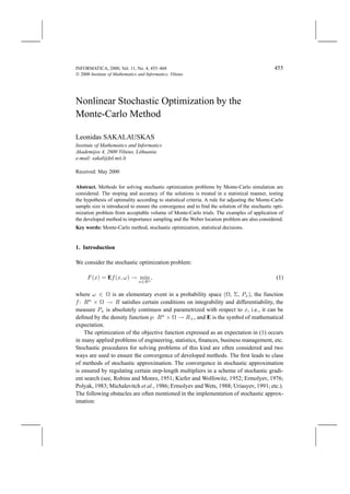
- 6. 460 L. Sakalauskas standard points could be introduced, considering the rate of convergence to the normal law and following from the Berry-Eseen or large deviations theorems. 4. Application to Importance Sampling Let us consider the aplication of the developed approach in the estimation of quantiles of the Gaussian distribution by importance sampling as an example. Let us apply the measure change procedure (Asmussen and Rubinstein, 1995): ∞ ∞ 1 − t2 2 1 (t−a)2 (t−a)2 t2 P (x) = √ e dt = √ e− 2 ·e 2 ·e− 2 dt 2π 2π x x ∞ ∞ 1 −at− a − t2 2 2 1 t2 = √ e 2 dt = √ g(a, t)e − 2 d t, (14) 2π 2π x−a x−a a2 where g(a, t) = e −at− 2 and find the second moment: ∞ ∞ 1 − t2 2 1 2 e −2at−a − t2 2 D (x, a) = √ 2 2 g (a, t)e dt = √ dt 2π 2π x−a x−a ∞ 2 ∞ 1 a2 2 ea t2 = √ e −at+ 2 − t2 dt = √ e − 2 d t. (15) 2π 2π x x+a Then the ratio D2 (x, a) − P 2 (x) δ2 = P (x) − P 2 (x) could be used as a measure of variance change (see Fig. 1). The variance of the Monte- Carlo estimator of the integral obtained can be reduced by fitting the parameter a. Let us differentiate with respect to a the last by one expression of D(x, a) in (15). The mimimum condition can be obtained after noncomplex manipulations by equating to zero the derivative and changing the: ∞ 2 te −2at−a − t2 2 √1 dt 2π x−a a= ∞ . (16) 2 e −2at−a − 2 2 t √1 dt 2π x−a
- 7. Nonlinear Stochastic Optimization by the Monte-Carlo Method 461 Fig. 1. Dependency of δ2 on the parameter of measure change a (x = 3). To demonstrate an approach to rationally choose the optimization step length, using the method of a simple iteration, consider the iterative procedure Nt i i=1 y H(y − x + a )g(a , y ) i t t i at+1 = Nt , i=1 H(y − x + a )g(a , y ) i t t i where y i are standard Gaussian variables, H(t) = 1, if t > 0, and H(t) = 0 in the opposite case. This can be used to solve (16) as a separate case of (7) when 1 ρt+1 = , Pt Nt 1 Pt = H(y i − x + at )g(at , y i ). (17) Nt i=1 This procces is iterated starting from a certain initial sample, changing the Monte-Carlo sample size according to (8) and stopping when estimate (17) is obtained with a permis- sible accuracy according to (13) and the hypothesis on the validity of condition (18) is not rejected according to criterion (12). Then the decision could be made: P (x) ≈ P t . The results of application of the procedure developed are given in Tables 1 and 2 for the cases x = 3 and x = 5, and initial data: a0 = x, N 0 = 1000, ε = 1%. We see that 4 and 3 series respectively were used to find the parameter for the optimal measure change. It is of interest to note that the optimization for x = 3 has been required 107 times fewer Monte-Carlo trials than with the number necessary to estimate probability (14) by the standard Monte-Carlo procedure and 497514 times fewer for x = 5, respectively. The Monte-Carlo estimators obtained can be be compared with those computed analythically.
- 8. 462 L. Sakalauskas Table 1 x=3 Proposed N t Generated N t Pt t At according to (8) according to (8) ε(%) P (x) = 1.34990 × 10⁻³ and (13) 1 3.000 1000 1000 10.692 1.52525 × 10⁻³ 2 3.154 9126 9126 3.770 1.34889 × 10⁻³ 3 3.151 35.8 × 10⁻⁶ 128327 1.000 1.34372 × 10⁻³ 4 3.156 64.8 × 10⁻⁶ 127555 1.000 1.35415 × 10⁻³ Table 2 x=5 Proposed N t Generated N t Pt t at according to (8) according to (8) ε(%) P (x) = 2.86650 × 10⁻⁷ and (13) 1 5.000 1000 1000 16.377 2.48182 × 10⁻⁷ 2 5.092 51219 51219 2.059 2.87169 × 10⁻⁷ 3 5.097 46.5 × 10⁻⁶ 217154 1.000 2.87010 × 10⁻⁷ 5. Stochastic Weber Problem As the next example, we consider the classical location problem, known as the Weber problem (Ermolyev and Wets, 1986; Uriasyev, 1990). The problem is as follows: find a point x on a plane minimizing the sum of weighted distances up to the given random points, distributed normally N (η k , dk ): K F (x) = βk |x − w| n(w, η k , dk )d w → min, k=1 R2 where βk = 1, . . . , K, (values of β k , η k , dk are given in (Uriasyev, 1990). We apply the method of simple iteration again. It is easy to see that: K ∂F x−w = βk n(w, η k , dk )d w. ∂x |x − w| k=1 R2 Equating this gradient to zero the equation of a “fixed point” for the optimal solution can be derived: K K wn(w, η k , dk ) n(w, η k , dk ) x+ = βk dw βk d w. |x+ − w| |x+ − w| k=1 R2 k=1 R2
- 9. Nonlinear Stochastic Optimization by the Monte-Carlo Method 463 Table 3 iterations number of trials Nt t min 5 1226 mean 10.45 3770 max 20 10640 Now the optimization procedure can be constructed by iteratively using this equation starting from a certain initial approximation x0 : K K wn(w, η k , dk ) n(w, η k , dk ) xt+1 = βk dw βk d w. (18) |xt − w| |xt − w| k=1 R2 k=1 R2 Substituting this expression into (7), we obtain that the corresponding step length as fol- lows: K n(w, η k , dk ) ρt+1 = 1 βk d w. |xt − w| k=1 R2 This problem was solved 400 times by means of algorithm (18) evaluating the in- tegrals by the Monte-Carlo method, adjusting the sample size according to rule (8), and stopping according to (12), (13). The initial data were as follows: x = (54, 30), N 0 = 10, β = 0.95, µ = 0.1, γ = 0.05. The optimum was found in all realizations with a permis- sible accuracy. The amount of computational resources, needed to solve the problem, is presented in Table 3. 6. Discussion and Conclusions An iterative method has been developed to solve the stochastic optimization problems by a finite sequence of Monte-Carlo samples. This method is grounded by the stopping pro- cedure (12), (13), and the rule for iterative regulation of size of Monte-Carlo samples (8). The proposed stopping procedure allows us to test the optimality hypothesis and to eval- uate the confidence intervals of the objective function in a statistical way. The regulation of sample size, when this size is taken inversely proportional to the square of the norm of the gradient of the Monte-Carlo estimate, allows us to solve stochastic optimization problems rationally from the computational viewpoint and guarantees the convergence almost surely at a linear rate. The examples confirm theoretical conclusions and show that the procedures developed permit solution of stochastic optimization problems with a sufficient permissible accuracy using an acceptable volume of computations.
- 10. 464 L. Sakalauskas Appendix Lemma 1. Let the conditions of Theorem 1 be valid. Then the inequality 2 ρ·L ρ·K EF x − ρ · G(x) F (x) − ρ · E G(x) 1− + , (1A) 2 N holds. Proof. We have from the Lagrange formula (Diedonne, 1960) that 1 F x − ρG(x) = F (x) − ρ G(x) F x − τ · ρ · G(x) d τ 0 2 2 = F (x) − ρ G(x) + ρ G(x) − F (x) +ρ ( F (x)) G(x) − F (x) 1 −ρ G(x) F x − τ · ρ · G(x) − F (x) d τ. (2A) 0 Formula (1A) follows if we take the expectation of both sides of (2A), apply the Lipshitz condition and the estimate 2 K E G(x) − F (x) , ∀x ∈ Rn , ∀N 1, (3A) N following, in its turn, from the independence of trials in the Monte-Carlo estimator (5). The lemma is proved. Proof of Theorem 1 ∞ ∞ Let { t }t=0 be a stream of σ-algebras generated by the sequence {xt }t=0 and let us introduce a random sequence ρ·K Vt = F (xt ) + . (4A) Nt 1 Assume 0 < ρ L. Then by virtue of (1A) and (3A) we have that ρ 2 1 E (Vt+1 | t−1 ) Vt − · E G(xt ) | t−1 +ρ · K · E | t−1 2 N t+1 ρ 2K 2 Vt − 1− E G(xt ) | t−1 , t = 1, 2, . . . . (5A) 2 C
- 11. Nonlinear Stochastic Optimization by the Monte-Carlo Method 465 It follows that Vt is a semimartingale when 2K < 1. Let C 4K. If now we take un- C conditional expectations of both sides of inequality (5A), then, after certain noncomplex manipulations we get that t ρ 2 EF (x0 ) − EF (xt+1 ) + 2 · ρ · K > E G(xk ) . 4 k=0 The left side of this inequality is bounded because F (xt+1 ) F + > −∞, and there- 2 2 fore lim E G(xt ) = 0. In such a case, lim | F (xt )| = 0 (mod(P )), because t→∞ t→∞ E | F (xt )|2 < E |G(xt )|2 . The proof of the theorem 1 is completed. Proof of Theorem 2 Let us introduce the Lyapunov function: 2 ρ·K W (x, N ) = x − x+ + . N We have by virtue of the Lagrange formula and (3A) that 2 E xt − x+ | t 2 =E xt − x+ − ρ · ( F (xt ) − F (x+ )) − ρ · (G(xt ) − F (xt )) | t 2 1 (1 − ρ · l)2 E xt − x+ | t−1 +ρ2·K ·E | t−1 . (6A) Nt Next, due to (8), the triangle inequality, and (3A) we get 2 1 E | F (xt ) − F (x+ )| K 1 E ·E + N t+1 C C Nt L2 2 K 1 ·E xt − x+ + ·E . (7A) C C Nt Note, we can change the conditional expectations in (6A) by unconditional. Thus, by virtue of (6A), (7A) we obtain: E W (xt+1 , N t+1 ) ρKL2 2 K 1 1−2ρl+ρ2l2 + E xt −x+ +ρK ρ+ E √ C C Nt K · L2 (1 − ρ · l − E W (xt , N t ) (8A) C 2 1 3 if 0 < ρ min L , 4·(1+l) ,C K max[4, L ]. The proof of the theorem 2 is com- l pleted.
- 12. 466 L. Sakalauskas References Antreich, K.J., R. Koblitz (1982). Design centering by yield prediction. IEEE Transactions on Circuits and Systems, CAS-29, pp. 88–95. Asmussen S., R.Y. Rubinstein (1995). Steady state rare events simulation in queueing models and its complexity properties. Advances in queueing, Probab Stochastics Ser., CRC, Boca Ruton, FL. pp. 429–461. Beliakov, Ju.N., F.A. Kourmayev, B.V. Batalov (1985). Methods of Statistical Processing of IC by Computer. Radio i Sviaz, Moscow (in Russian). Bentkus, V., F. Gotze (1999). Optimal bounds in non-Gaussian limit theorems for U-statistics. Annals of Prob- ability, 27(1), 454–521. Bhattacharya, R.N., R. Ranga Rao (1976). Normal Approximation and Asymptotic Expansions. John Wiley, New York, London, Toronto. Box, G., G. Watson (1962). Robustness to non-normality of regression tests. Biometrika, 49, 93–106. Dieudonne, J. (1960). Foundations of Modern Analysis. Academic Press, N.Y., London. Ermolyev, Ju.M. (1976). Methods of Stochastic Programming. Nauka, Moscow (in Russian). Ermolyev, Yu., R. Wets (1988). Numerical Techniques for Stochastic Optimization. Springer-Verlag, Berlin. Ermolyev, Yu., I. Norkin (1995). On nonsmooth problems of stochastic systems optimization. WP–95–96, IIASA, A-2361, Laxenburg, Austria. Feller, W. (1966). An Introduction to Probability Theory and its Applications, vol. II. Wiley, New-York. Jun Shao (1989). Monte-Carlo approximations in Bayessian decision theory. JASA, 84(407), 727–732. Katkovnik, V.J. (1976). Linear Estimators and Problems of Stochastic Optimization. Nauka, Moscow (in Rus- sian). Kantorovitch, L., G. Akilov (1959). Functional Analysis in Normed Spaces. Fizmatgiz, Moscow (in Russian). Kiefer, J., J. Wolfowitz (1952). A stochastic estimation of the maximum of a regression function. Annals of Mathematical Statistics, 23(3), 462–466. Krishnaiah, P.R. (1988). Handbook of Statistics. Vol. 1, Analysis of Variance. North-Holland, N.Y.- Amsterdamm. Mikhalevitch, V.S., A.M. Gupal and V.I. Norkin (1987). Methods of Nonconvex Optimization. Nauka, Moscow (in Russian). Pflug, G.Ch. (1988). Step size rules, stopping times and their implementation in stochastic optimization algo- rithms. In Ju. Ermolyev and R. Wets (Eds.), Numerical Techniques for Stochastic Optimization. Springer- Verlag, Berlin, pp. 353–372. Polyak, B.T. (1983). Introduction to Optimization. Nauka, Moscow (in Russian). Robins, H., and S. Monro (1951). A stochastic approximation method. Annals of Mathematical Statistics, 3(22), 400–407. Rubinstein, R. (1983). Smoothed functionals in stochastic optimization. Mathematical Operations Research, 8, 26–33. Sakalauskas, L. (1992). System for statistical simulation and optimization of linear hybrid circuits. Proc. of the 6th European Conference on Mathematics in Industry (ECMI’91), August 27–31, 1991, Limerick, Ireland, Teubner, Stuttgart, 259–262. Sakalauskas, L.L., S. Steishunas (1993). Stochastic optimization method based on the Monte-Carlo simulation. Proc. Intern. AMSE Conference “Applied Modelling and Simulation”, Lviv (Ukraine), Sept. 30–Oct. 2, 1993, AMSE Press, 19–23. Sakalauskas, L. (1997). A centering by the Monte-Carlo method. Stochastic Analysis and Applications, 4(15). Shapiro, A. (1989). Asymptotic properties of statistical estimators in stochastic programming. The Annals of Statistics, 2(17), 841–858. Uriasjev, S.P. (1990). Adaptive algorithms of stochastic optimization and theory of games. Nauka, Moscow (in Russian). Yudin, D.B. (1965). Qualitative methods for analysis of complex systems. Izv. AN SSSR, ser. Technicheskaya Kibernetika, 1, 3–13 (in Russian).
- 13. Nonlinear Stochastic Optimization by the Monte-Carlo Method 467 L. Sakalauskas has graduated from the Kaunas Polytechnic Institute (1970), received the PhD degree from this Institute (1974), Associated Professor (1987), Member of the New- York Academy of Sciences (1997), presently is a Head of the Statistical Modelling Group at the Institute of Mathematics and Informatics and an Associated Professor of the Transport Engineering Department of the Vilnius Gediminas Technical University.
- 14. 468 L. Sakalauskas Netiesinis stochastinis optimizavimas Monte-Karlo metodu Leonidas Sakalauskas Nagrin˙ jami Monte-Karlo tipo proced¯ ru taikymai stochastinio optimizavimo uždaviniams spresti. e u Metodo stabdymo taisykl˙ s ir sprendinio tikslumas yra nustatomi statistiniu b¯ du, tikrinant e u statistine optimalumo hipoteze. Ivesta Monte-Karlo imˇ iu dydžio parinkimo taisykl˙ , užtikrinanti c e konvergavima bei stochastio optimizavimo problemos sprendima po baigtinio, praktiniu poži¯ riuu dažnai priimtino, Monte-Karlo bandymu skaiˇ iaus. Pasi¯ lytas metodas pritaikytas sprendžiant c u reikšmingu imˇ iu ir stochastine Veberio problema. c