SlideShare ist ein Scribd-Unternehmen logo
1 von 44
Downloaden Sie, um offline zu lesen
Schnappverbindungen
und Federelemente
aus Kunststoff
Snap Joints
and springs
in Plastics
Allgemein/
General
Anwendungstechnische
Information
Application Technology
Information
ATI
1119
d, e
Ersetzt Ausgabe 1999-10-01
Replaces edition of 1999-10-01
A. Maszewski
Geschäftsbereich
Kunststoffe
Plastics
Business Group
2
Inhaltsverzeichnis: Seite
Formel-Zeichen und Begriffe 3
1. Grundsätzliches 4
1.1 Allgemeine Beschreibung 4
1.2 Ausführungsarten 4
1.3 Allgemeine Auslegungshinweise 5
1.3.1 Belastungsverhältnisse 5
1.3.2 Beanspruchung 5
1.3.3 Relaxation – Retardation 6
1.3.4 Kerbwirkung 7
1.4 Verteilung der Auslenkung auf die
Fügepartner 7
1.5 Zulässige Auslenkung 8
1.5.1 Zulässige Dehnung 9
1.5.2 Zulässige Torsionsspannung 10
1.6 Auslenkkraft 11
1.7 Fügekraft 13
1.8 Reibungskoeffizienten 13
1.9 Gestaltungshinweise 14
2. Schnapparmverbindungen 15
2.1 Berechnungsgrundlagen 15
2.2 Berechnungsbeispiel 19
2.3 Anwendungsbeispiele 21
3. Torsionsschnappverbindungen 23
3.1 Berechnungsgrundlagen 23
3.2 Berechnungsbeispiel 24
3.3 Anwendungsbeispiele 27
4. Ringschnappverbindungen 28
4.1 Berechnungsgrundlagen 28
4.2 Berechnungsbeispiel 31
4.3 Anwendungsbeispiele 33
5. Ringförmige Schnappverbindungen 34
5.1 Berechnungsgrundlagen 34
5.2 Berechnungsbeispiel einer
ringartigen Schnappverbindung 40
6. Literaturhinweise 43
Table of contents Page
Symbols 3
1. Basic information 4
1.1 General description 4
1.2 Types of snap joint 4
1.3 General design advice 5
1.3.1 Loading conditions 5
1.3.2 Loading 5
1.3.3 Relaxation - retardation 6
1.3.4 Notch effect 7
1.4 Dividing up the deflection over the
mating parts 7
1.5 Permitted deflection 8
1.5.1 Permitted strain 9
1.5.2 Permitted torsional stress 10
1.6 Deflection force 11
1.7 Mating force 13
1.8 Coefficients of friction 13
1.9 Design advice 14
2. Cantilever snap arm joints 15
2.1 Design and calculation criteria 15
2.2 Calculation example 19
2.3 Sample applications 21
3. Torsion snap joints 23
3.1 Design and calculation criteria 23
3.2 Calculation example 24
3.3 Sample applications 27
4. Annular snap joints 28
4.1 Design and calculation criteria 28
4.2 Calculation example 31
4.3 Sample applications 33
5. Ring-shaped snap joints 34
5.1 Design and calculation criteria 34
5.2 Calculation example for a ring-shaped
snap joint 40
6. Literature 43
3
Symbols
a dimensions
B width of the undercut
b width of profile
C geometric factor for ring segments
d diameter at the joint
da outer diameter (hub)
di inner diameter (shaft)
Eo elastic modulus (tangential intrinsic modulus)
Es secant modulus
e distance between outer fibre and neutral axis
F mating force
f undercut, deflection
G shear modulus
h height of profile
K geometric factor for torsion cross-sections
L length of the edge
l length of lever arm
Q deflection force
R friction force
r radius
s wall thickness
W axial section modulus
Wp section modulus of torsion
X geometric factor for annular snap joint
Index W = shaft, Index N = hub
α angle of inclination
β angle of twist
γ shear strain
δ distance of snap-fitting groove from end
ε elongation
εzul maximum permissible strain
εR elongation at break
εS yield strain
µ friction coefficient
ν poisson’s ratio
ρ friction angle
σ stress
ϕ segment angle
Formelzeichen und Begriffe
a Abmessungen
B Hinterschnitt-Breite
b Profilbreite
C Geometriefaktor für Kreisbogensegmente
d Durchmesser an der Fügestelle
da Außendurchmesser (Nabe)
di Innendurchmesser (Welle)
Eo E-Modul (Tangenten-Ursprungs-Modul)
Es Sekanten-Modul
e Randfaserabstand von neutr. Faser
F Fügekraft
f Hinterschnitt, Auslenkungn
G Schubmodul
h Profilhöhe
K Geometriefaktor für Torsionsquerschnitte
L Kantenlänge
l Hebelarmlänge
Q Auslenkkraft
R Reibungskraft
r Radius
s Wanddicke
W axiales Widerstandsmoment
Wp polares Widerstandsmoment
X Geometriefaktor für Ringschnappverbindung
Index W = Welle, Index N = Nab
α Schrägungswinkel
β Auslenkwinkel
γ Scherung
δ Abstand der Schnappnut vom Ende
ε Dehnung
εzul max. zulässige Dehnung
εR Reißdehnung
εS Streckdehnung
µ Reibungskoeffizient
ν Querkontraktionszahl
ρ Reibungswinkel
σ Spannung
ϕ Segmentwinkel
4
1 Grundsätzliches
1.1 Allgemeine Beschreibung
Schnappverbindungen stellen eine einfache und kostengünstige
Art der Verbindungstechnik dar. Sie sind charakteristisch für die
Werkstoffgruppe der Kunststoffe, da deren Werkstoffeigen-
schaften (Flexibilität) und Formgebungsmöglichkeiten ihrer
Realisierung besonders entgegen kommen.
Grundsätzlich sind Schnappverbindungen aus einem elastischen
Federelement und einer Rastvorrichtung (Hinterschnitt) aufge-
baut. Ihre Funktion teilt sich in den Füge- bzw. Löse- sowie den
Haltevorgang.
1.2 Ausführungsarten
Die Schnappverbindungen werden nach der Art des Feder-
elements und nach der Lösbarkeit der Verbindung eingeteilt.
Es wird grundsätzlich zwischen
a) den Schnapparmverbindungen (Biegebalkenprinzip),
b) den Torsionsschnappverbindungen (Torsionsstabprinzip),
c) den Ringschnappverbindungen (zylindrische Profile) und
d) den ringartigen Schnappverbindungen (regelmäßige
Polygonprofile)
unterschieden. In Abb. 1 sind diese vier Prinzipien schematisch
dargestellt.
1. Basic information
1.1 General description
Snap joints are a simple and inexpensive joining technique. They
are a characteristic type of joint used for polymer materials,
since the material properties (flexibility) and moulding poten-
tial of polymers are particularly conducive to this kind of
connection.
Snap joints are essentially made up of an elastic spring element
and a click-stop device (undercut). They serve the purpose of
joining or separating parts and holding them together.
1.2 Types of snap joint
Snap joints are classified according to the type of spring element
and the separability of the joint. A basic distinction is drawn
between
a) the snap arm joint (flexural beam principle)
b) the torsional snap joint (torsion rod principle)
c) the annular snap joint (cylindrical profiles)
d) the ring-shaped snap joint (regular polygon profiles)
These four principles are shown in diagram form in Fig. 1.
Fig. 1: Types of snap jointAbb. 1: Schnappverbindungsarten
a) b)
c) d)
5
In Abhängigkeit vom Hinterschnittwinkel wird außerdem noch
zwischen lösbaren und unlösbaren Schnappverbindungen unter-
schieden (Abb. 2).
A distinction is also made between separable and inseparable
joints, as a function of the undercut angle (Fig. 2).
Fig. 2: Separable and inseparable jointAbb. 2: Lösbare und unlösbare Schnappverbindungen
1.3 Allgemeine Auslegungshinweise
Die Auslegung einer Schnappverbindung beinhaltet eine opti-
male Abstimmung der Konstruktion auf den Werkstoff. Hierzu
ist die genaue Kenntnis der Belastungsverhältnisse und der
Werkstoffeigenschaften erforderlich.
1.3.1 Belastungsverhältnisse
Die Belastungsverhältnisse einer Schnappverbindung unter-
scheiden sich grundlegend in Abhängigkeit von der Funktion.
Während der Fügevorgang in der Regel eine einmalige oder
mehrmalige kurzzeitige Belastung darstellt, bei der der
Werkstoff relativ hoch beansprucht werden darf, wird die
Haltefunktion meist von einer statischen Langzeit- oder gar
Dauerbelastung bestimmt, die eine deutlich geringere maxi-
male Beanspruchung zulässt. D. h., die Auslegung muss sowohl
den Füge- bzw. Löse- als auch den Haltevorgang umfassen.
1.3.2 Beanspruchung
Bei der Auslegung darf nicht vergessen werden, dass die Belas-
tung sowohl beim Füge- als auch beim Haltevorgang meist zu
mehreren überlagerten Lastfällen führt (z.B. Zug-, Scher- und
Biegebelastung), die in ihrer Wechselwirkung (Vergleichsspan-
nung bzw. -dehnung) berücksichtigt werden müssen.
Ab einem Verhältnis der Schnapparmlänge zu seiner Höhe von
kleiner als 5, sollte der Anteil der Schubverformung nicht
unberücksichtigt bleiben.
1.3 General design advice
The layout of a snap joint involves optimally tailoring the design
to the material. This requires precise knowledge of the loading
conditions and the material properties.
1.3.1 Loading conditions
The loading conditions for a snap joint differ fundamentally as
a function of the purpose that the snap joint serves. While the
joining operation generally imposes once-only or repeated short-
term load, during which time the material can be subjected to
a relatively high load level, the retaining function generally
involves a static long-term or even permanent load, where the
maximum permitted load is considerably lower. In other words,
the layout must be based on the joining and separation operation
as well as on the retaining function.
1.3.2 Loading
When conducting the layout, it must be remembered that both
the joining and the retaining operation generally involve a
number of different load cases being superimposed on each other
(e.g. tensile, shear and flexural load), and it is necessary to make
allowance for the interaction of these loads (effective stress,
effective strain).
Where the ratio of the snap arm length to the snap arm height is
smaller than 5, consideration must also be paid to the shear
deformation component.
6
1.3.3 Relaxation – retardation
In order to make allowance for the time-dependent behaviour of
the mechanical properties of plastics, it is important to achieve
a stress-free and positive-action connection as far as possible
(a form-fit rather than a friction-lock joint). If this is not
entirely possible, then allowance can be made for
– relaxation: stress falls over time with constant strain or
– retardation: strain increases over time with constant stress
with the aid of isochronous stress-strain curves. Information on
this is shown in graphic form in Fig. 4.
1.3.3 Relaxation – Retardation
Um dem zeitabhängigen Verhalten der mechanischen Eigen-
schaften von Kunststoffen Rechnung zu tragen, sollte nach dem
Einrasten eine möglichst entspannte und formschlüssige Ver-
bindung (Formschluss vor Kraftschluss) angestrebt werden.
Ist dies nicht vollständig möglich, so kann
– die Relaxation: Spannung fällt bei konstanter Dehnung mit
der Zeit ab oder
– die Retardation: Dehnung nimmt bei konstanter Spannung
mit der Zeit zu
anhand von isochronen Spannungs-Dehnungs-Kurven berück-
sichtigt werden. In Abb. 4 sind entsprechende Hinweise hierzu
graphisch dargestellt.
Biegespannung / Bending stress: σb =
Mb
W
=
Zugspannung / Tensile stress: σz =
F
A
=
F
b · h
= 0.5 ·
F
h2
z
Scherspannung / Shear stress: τs =
F
A
=
F
a · b
= 0.42 ·
F
h2
s
σb ÷ 6 ÷ 1 ÷ 0.84σz τs÷ =
Schlussfolgerung: Biegebeanspruchung ist meist die dominierende Beanspruchungsart.
Conclusion: Bending stress is mostly the dominant stress type.
Beispiel der Beanspruchung eines Schnapparms durch die Haltekraft (FH)/
Example of the stress status of a cantilever arm by cohesion (FH)
a = 1.2 · h, b = 2 · h, lm = h
F · l
b · h
m
2
= 3 ·
F
h2
6 ·
Abb. 3: Zusammengesetzte Beanspruchung Fig. 3: The combined loads that act
h
b
a
lm
neutrale faser
neutral fibre
FH
7
1.3.4 Kerbwirkung
Ein nach wie vor relativ häufiger Konstruktionsfehler betrifft
die Kerbwirkung. Besonders deutlich macht sich dieser Fehler
bei amorphen Werkstoffen bemerkbar. Aus diesem Grund wird
hier ausdrücklich auf die Notwendigkeit der Abrundung von
Ecken und Kanten bzw. der Vermeidung von Gratbildung in den
beanspruchten Bereichen hingewiesen. Als günstig hat sich in
der Praxis ein Kerbradius von 0,5 mm erwiesen. In Abb. 5 ist der
Zusammenhang zwischen dem Kerbradius und der Spannung
exemplarisch dargestellt.
1.4 Verteilung der Auslenkung auf die Fügepartner
Im ungünstigsten Fall muss einer der beiden Fügepartner um den
Gesamtbetrag der Auslenkung (Hinterschnitt) verformt werden.
Tatsächlich verteilt sich die Verformung in der Regel auf beide
Fügepartner.
Die Verformungsverteilung auf die Fügepartner kann am ein-
fachsten graphisch ermittelt werden. Hierzu muss für jeden der
beiden Fügepartner zuerst ein Kraft-Verformungs-Diagramm
(Federkennlinie), wie in Abb. 6 dargestellt, bestimmt werden.
Die Überlagerung beider Federkennlinien ergibt einen Schnitt-
punkt, der die tatsächliche Auslenkkraft und die Verformungs-
anteile beider Fügepartner angibt.
1.3.4 Notch effect
One design error still committed fairly frequently relates to the
notch effect. This error is particularly noticeable with amor-
phous materials. For this reason, the importance of rounding
corners and edges and avoiding flash in areas subject to load
must be stressed here. A notch radius of 0.5 mm has proved
favourable in practice. Figure 5 shows the correlation between
the notch radius and the stress on the basis of an example.
1.4 Dividing up the deflection over the mating parts
In the least favourable case, one of the two mating parts needs
to be deformed by the full amount of the deflection (undercut).
As a rule, however, the deformation will be divided over both the
mating parts.
The easiest way to establish the distribution of the deformation
over the mating parts is on a graph. To do this, it is first necess-
ary for a force-deformation diagram (spring characteristic) to be
established for each of the two mating parts, as shown in Fig. 6.
By superimposing the two spring characteristics, a point of
intersection is obtained which indicates the actual deflection
force and the deformation components of the two mating parts.
Abb. 4: Relaxation und Retardation (Kriechen) Fig. 4: Relaxation and retardation (creep)
8
Abb. 5: Spannung in Abhängigkeit vom Kerbradius bei
gleicher Verformung
Fig. 5: Stress versus the notch radius for identical
deformation
Bei Torsionsschnappverbindungen setzt sich die Gesamtver-
formung des Torsionsarms aus der Drillverformung und aus der
Biegeverformung zusammen. Oft kann der Anteil der Biege-
verformung zwar vernachlässigt, er soll jedoch nicht vergessen
werden. Abgesehen davon, muss die Biegeverformung des
Betätigungshebels bei der Auslegung des Betätigungsweges
(Anschlag) berücksichtigt werden.
Für die Ringschnappverbindungen sind entsprechende Feder-
kennlinien in Abb. 28 dargestellt. Hierbei wird davon ausge-
gangen, dass wegen der Zugbeanspruchung bzw. der Dehnung
(= versagensrelevante Größe) die Nabe der auszulegende Füge-
partner ist und die Gesamtverformung (Hinterschnitt) aufzu-
nehmen hat (Nabe flexibel – Welle starr). Trifft dies nicht zu, ist
die tatsächliche Werkstoffbeanspruchung entsprechend gerin-
ger. Bei gleich steifen Fügepartnern halbiert sich die Beanspru-
chung, d. h., der zulässige Hinterschnitt ist doppelt so groß wie
bei starr angenommener Welle.
1.5 Zulässige Auslenkung
Die zulässige Auslenkung f (zulässiger Hinterschnitt) kann in
Abhängigkeit von der zulässigen Dehnung des verwendeten
Werkstoffs berechnet werden. Sie soll weder beim Einschnapp-
vorgang noch bei der gewaltsamen Entformung aus dem Spritz-
gießwerkzeug (Temperatur!) überschritten werden.
In the case of torsional snap joints, the overall deformation of
the torsion arm is made up of the twisting deformation and the
flexural deformation. In many cases it is possible to neglect the
flexural deformation component, but it should not be forgotten.
Apart from this, allowance must be made for the flexural defor-
mation of the actuating arm when designing the actuating path
(catch).
Corresponding spring characteristics are set out in Fig. 28 for
annular snap joints. It is assumed here, on the basis of the tensile
stressing or strain (= parameter of relevance for failure), that the
hub is the mating part that is to be designed and this has to
absorb the overall deformation (undercut), i.e. the hub is flexible
and the shaft rigid. If this is not the case, the actual load acting
on the material will be correspondingly smaller. With mating
parts of identical rigidity, the load is halved, in other words,
the permitted undercut is twice as big as for a shaft assumed to
be rigid.
1.5 Permitted deflection
The permitted deflection f (permitted undercut) can be calcu-
lated as a function of the permitted strain of the material being
used. This should not be exceeded during the snap-in opera-
tion or during removal from the injection mould (attention to be
paid to the temperature).
9
1.5.1 Zulässige Dehnung
Beim Fehlen genauer Angaben kann die zulässige Dehnung oder
Spannung bei einer einmaligen kurzzeitigen Auslenkung bei
23 °C anhand der folgenden Regel abgeschätzt werden:
q nahezu die Streckdehnung bei teilkristallinen Thermoplasten
q ca. 70% der Streckdehnung bei amorphen Thermoplasten
q ca. 50 % der Bruchdehnung bei glasfaserverstärkten Thermo-
plasten
In Abb. 7 ist dieser Zusammenhang graphisch dargestellt.
1.5.1 Permitted strain
If precise data is not available, the permitted strain or stress
for a brief, once-only deflection at 23 °C can be estimated by
using the following rule:
q almost the tensile strain at yield for semi-crystalline thermo-
plastics
q approx. 70% of the tensile strain at yield for amorphous
thermoplastics
q approx. 50% of the tensile strain at break for glass-fibre rein-
forced thermoplastics
This relationship is depicted in graph form in Fig. 7.
Abb. 6: Verteilung der Auslenkung auf die Fügepartner
Abb. 7: Bestimmung der zulässigen Dehnung für den
Einschnappvorgang (links: Werkstoff mit aus-
geprägter Streckgrenze; rechts: glasfaserver-
stärkter Werkstoff ohne Streckgrenze)
Fig. 7: Determination of the permitted strain for the
snap-in operation (left: material with a distinct
yield point; right: glass fibre reinforced material
without a yield point)
Fig. 6: Distribution of the deflection of the mating parts
a) Fügepartner / Mating part 1
Federweg / Deflection
0 1/3f 2/3f f
Querkraft/TransverseforceQ
b) Fügepartner / Mating part 2
01/3f2/3ff
Querkraft/TransverseforceQ
c) Fügepartner / Mating parts 1 + 2
gesamter Federweg f = Hinterschnitt /
total deflection f = untercut
tatsächl.
Auslenkkraft/
realdeflection
forceQ
Federweg/
Deflection f1
Federweg/
Deflection f2
=+
Federweg / Deflection
Spannung/Stressσ
Dehnung / Strain ε
0.7 x εs εs
Spannung/Stressσ
Dehnung / Strain ε
0.5 x εB εB
amorph /
amorphous
teilkristallin /
semi-crystalline
GF-Produkte /
GRP products
10
Für einige Werkstoffe sind die zulässigen Dehnungen für eine
einmalige kurzzeitige Belastung als Richtwerte (in %) in Tab. 1
aufgeführt:
Table 1 shows the permitted strains for brief, once-only loading
for a number of materials. These values are guide values, given
in percent.
teilkristallin / amorph / glasfaserverstärkt /
semi-crystalline amorphous glass fibre reinforced
PE 8% PC 4% PA 6-GF~ 2.0%
PP 6% (PC+ABS) 3% PA 6-GF^ 1.5%
PA ~ 6% ABS 2.5% PC-GF 1.8%
PA ^ 4% CAB 2.5% PBTP-GF 1.5%
POM 6% PVC 2% ABS-GF 1.2%
PBTP 5% PS 1.8%
~ : konditioniert / conditioned,
^ : spritzfrisch / as moulded
Bei häufiger kurzzeitiger Betätigung kann in etwa von ca. 60 %
der einmalig zulässigen Werte ausgegangen werden.
Bei Langzeit- oder Dauerbelastung besteht bei amorphen Pro-
dukten die Gefahr der Spannungsrissbildung. Sie muss geson-
dert berücksichtigt werden. Untersuchungen haben gezeigt, dass
bei Dehnungen unterhalb ca. 0,5 % die Spannungsrissgefahr
(bei 23 °C in Luft) deutlich geringer ist.
Eine differenziertere Abschätzung von zulässigen Bemes-
sungskennwerten vieler Bayer-Thermoplaste unter Berücksich-
tigung der Belastungsdauer, der Temperatur, der Belastungsart,
der Orientierung, der Bindenaht usw. erlaubt das Programm
„RALPH“ , das unter der folgenden Adresse angefordert werden
kann: Bayer-AG, KU-EU/INFO, Geb. B 207, 51368 Leverkusen.
1.5.2 Zulässige Torsionsspannung
Bei Torsionsbelastung entsteht Schubbeanspruchung. Die zuläs-
sige Torsionsschubspannung τzul kann für die meisten Kunst-
stoffe überschlägig nach der folgenden Beziehung abgeschätzt
werden:
With frequent brief actuation, it is possible to work on the basis
of approx. 60 % of the permitted values for once-only actuation.
With long-term or permanent load, there is a danger of stress
cracking with amorphous products. Extra allowance must be
made for this. Studies have shown that the danger of stress
cracking (at 23 °C in air) is considerably lower with a strain of
less than around 0.5 %.
The “RALPH” program permits a differentiated estimate of
permitted dimensioning values for a large number of Bayer
thermoplastics, making allowance for the loading duration, the
temperature, the nature of the loading, the orientation and the
weld line, etc. This program may be ordered from: Bayer-AG,
KU-EU/INFO, Geb. B 207, D-51368 Leverkusen.
1.5.2 Permitted torsional stress
Shear stressing results under torsional load. The permitted
torsional shear stress τzul can be estimated on an approximate
basis for the majority of plastics with the following relationship:
Tab. 1: Richtwerte für zulässige Dehnungen bei
einmaliger kurzzeitiger Belastung
Table 1: Guide values for permitted strains for brief,
once-only loading
11
Die Querkontraktionszahlen „ν“ (= Poisson-Zahlen) liegen bei
gängigen Thermoplasten im Bereich von ca. 0,33 – 0,45. Der
untere Wert gilt hierbei für hoch glasfaserverstärkte und der
obere für hoch elastomermodifizierte Thermoplaste. Beim
Fehlen genauer Angaben wird oft ein Wert von 0,35 benutzt.
Mit der linearen Mischungsregel kann für den zeit- und tempe-
raturabhängigen Sekantenmodul ES eine entsprechende Quer-
kontraktionszahl bestimmt werden.
The Poisson's ratios “ν” are between some 0.33 and 0.45 for
commonly-used thermoplastics. The lower value here applies for
thermoplastics with a high level of glass fibre reinforcement and
the upper value for highly elastomer-modified thermoplastics.
If a precise figure is not available, a value of 0.35 is frequently
used.
Applying the linear mixing rule, it is possible to determine
an appropriate Poisson's ratio for the time and temperature-
dependent secant modulus, ES.
Abb. 8: Ermittlung des Sekanten-Moduls Fig. 8: Determination of the secant modulus
Spannung/Stressσ
Dehnung / Strain ε
E0
εl
Sekanten-Modul /
Secant modulus
ES
ES =
σl
ε1
σl
1.6 Auslenkkraft
Die Auslenkkraft kann in Abhängigkeit von der geometrischen
Steifigkeit (Querschnittgestaltung), der zulässigen Dehnung und
der Werkstoffsteifigkeit (E-Modul) entsprechenden berechnet
werden.
Da die beim Fügevorgang auftretenden Dehnungen oft außer-
halb des Proportionalitäsbereichs der Spannungs-Dehnungs-
Kurve liegen, sollte der Genauigkeit wegen, anstatt des Elasti-
zitätsmoduls der sogenannte „Sekanten-Modul“ (= dehnungs-
abhängiger Elastizitätsmodul) für die Bestimmung der Aus-
lenkkraft verwendet werden. Seine Ermittlung ist in Abb. 8 dar-
gestellt. Hierbei ist immer jene Dehnung einzusetzen, die für die
erforderliche Auslenkung ermittelt wurde.
Für einige Bayer-Thermoplaste ist der Sekanten-Modul in
Abhängigkeit von der Dehnung in Abb. 9 dargestellt.
1.6 Deflection force
The deflection force can be calculated as a function of the geo-
metrical rigidity (cross-sectional shape), the permitted strain,
and the rigidity of the material (Young’s modulus).
Since the strains that occur during the joining operation are fre-
quently outside the proportionality range of the stress-strain
curve, the so-called “secant modulus” (= strain-dependent
Young’s modulus) should be used instead of the Young's modu-
lus, since this will allow the deflection force to be determined
more accurately. Figure 8 shows how this is established. The
strain determined for the requisite deflection must always be
entered here.
The secant modulus for a number of Bayer thermoplastics is
shown in Fig. 9 as a function of strain.
12
Abb. 9: Sekantenmoduli einiger Bayer-Thermoplaste Fig. 9: Secant moduli of a number of Bayer thermo-
plastics
16000
MPa
12000
10000
8000
6000
4000
2000
0
0 0,5 11 1,5 2 2,5 3 % 4
Dehnung / Strain
Sekantenmodul/Secantmodulus
Durethan B
BKV 50 H1.0 ^
BKV 30 H1.0 ^
BKV 50 H1.0 ~
BKV 15 H1.0 ~
B 30 S ~
B 30 S ^
BKV 30 H1.0 ~
BKV 15 H1.0 ^
^ = spritzfrisch
~ = konditioniert
* Versuchsprodukt s. Prospektrückseite
^ = as moulded
~ = conditioned
* Trial product see back page
13
1.7 Fügekraft
Bei der Montage müssen die Auslenkkraft Q und die Reibungs-
kraft R überwunden werden (Abb. 10).
Die Fügekraft F ergibt sich aus:
Bei lösbaren Verbindungen kann analog der Fügekraft auch die
Lösekraft bestimmt werden. In diesem Fall ist der Neigungs-
winkel der Löseflanke α’ in die obige Gleichung einzusetzen.
Bedingt durch die stark schwankenden Reibungsverhältnisse,
können die Fügekräfte in der Regel nur mit einer entsprechend
großen Toleranz abgeschätzt werden.
1.7 Mating force
When the parts are joined, the deflection force Q and the fric-
tion force R have to be overcome (Fig. 10).
The mating force F is obtained from
With separable joints, the separation force can be determined in
the same way as the mating force. In this case, the angle of
inclination to be introduced into the above equation is the angle
of the separation side, α’. The highly fluctuating friction
conditions mean that the mating forces can generally only be
estimated with a correspondingly high tolerance.
Abb. 10: Zusammenhang Auslenkkraft – Fügekraft
Tab. 2: Richtwerte für Gleitreibungskoeffizienten Table 2: Guide values for coefficients of sliding friction
1.8 Reibungskoeffizienten
In Tab. 2 sind einige Anhaltswerte für Gleitreibungskoeffizi-
enten für die Reibpaarung Kunststoff – Stahl aufgeführt. Sie
sind der Literatur entnommen. Bei einer Paarung Kunststoff -
anderer Kunststoff kann (nach VDI 2541) mit gleichen oder
etwas niedrigeren Werten gerechnet werden, wie in der unteren
Tabelle angegeben. Bei gleichen Reibungspartnern ist meist mit
höheren Reibungskoeffizienten zu rechnen. Soweit bekannt, sind
die entsprechenden Werte in Tab. 2 angegeben.
Fig. 10: Relationship between deflection force and
mating force
1.8 Coefficients of friction
Table 2 shows a number of guide values for the coefficients of
sliding friction for the friction combination of plastic and steel.
These have been taken from the literature. Where a plastic is
combined with a dissimilar plastic, it is possible to use the same
or slightly lower values, according to VDI 2541, as is shown
in the Table below. Where the two parts are made of the same
material, then higher coefficients of friction must generally be
expected. The corresponding values are given in Table 2 insofar
as they are known.
Reibungskoeffizienten / Coefficients of friction
Werkstoff / Kunststoff – Stahl / Gleiche Reibungspartner /
Material Plastic – Steel Identical friction partners
PTFE 0.12 – 0.22 0.12 – 0.22
PE-HD 0.20 – 0.25 0.40 – 0.50
PP 0.25 – 0.30 0.38 – 0.45
POM 0.20 – 0.35 0.30 – 0.53
PA 0.30 – 0.40 0.45 – 0.60
PBTP 0.35 – 0.40 –
PS 0.40 – 0.50 0.48 – 0.60
SAN 0.45 – 0.55 –
PC 0.45 – 0.55 0.54 – 0.66
PMMA 0.50 – 0.60 0.60 – 0.72
ABS 0.50 – 0.65 0.60 – 0.78
PE-LD 0.55 – 0.60 0.66 – 0.72
PVC 0.55 – 0.60 0.55 – 0.60
14
Abgesehen davon sind die Reibungskoeffizienten abhängig von
der Gleitgeschwindigkeit, dem Anpressdruck und der Ober-
flächenbeschaffenheit, was durch eine entsprechende Toleranz
berücksichtigt werden sollte.
1.9 Gestaltung:
Um möglichst große Hinterschnitte (= Fügesicherheit) reali-
sieren zu können, bedarf es optimaler Formgestaltung. Sie bein-
haltet hauptsächlich die Wahl der Querschnittsform und des
Querschnittsverlaufs des Federelements.
Die Querschnittsform wird durch die maßgebliche Belastungs-
art (beim Füge- oder Haltevorgang) bestimmt. Als optimal sind
hierbei folgende Querschnittsformen und Ausführungen anzu-
sehen:
q Zugbelastung
³ konstanter Rechteckquerschnitt
(s. Abb. 13, Ausführung 1)
q Biegebelastung
³ verjüngter Rechteckquerschnitt
(s. Abb. 13, Ausführung 2 oder 3)
q Torsionsbelastung
³ konstanter Kreisquerschnitt
Das Optimum kann u. U. erst durch eine Kombination der o.g.
Querschnittsformen und/oder ihrer Ausführungsarten erreicht
werden.
Alle anderen Querschnittsformen und -verläufe stellen Kom-
promisslösungen dar. Die Wahl des optimalen Querschnitts kann
neben den mechanischen Aspekten auch z. B. durch fließtech-
nische (Fließweg) Belange mitbestimmt werden.
In addition to this, the coefficients of friction are conditioned by
the sliding velocity, the contact pressure and the surface finish.
Allowance should be made for this through the corresponding
tolerance.
1.9 Design advice
In order to achieve the biggest possible undercuts (= secure
joint), it is essential to ensure the optimum design. This essen-
tially involves selecting the cross-sectional shape and the cross-
sectional profile of the spring element.
The cross-sectional shape is determined by the decisive load
type (during the mating or retaining operation). The optimum
cross-sectional shapes and designs are as follows:
q tensile load
³ constant square cross-section
(see Fig. 13, design type 1)
q flexural load
³ tapered square cross-section
(see Fig. 13, design type 2 or 3)
q torsional load
³ constant circular cross-section
In certain cases, the optimum design can only be achieved by
combining the above cross-sectional shapes and/or design types.
All other cross-sectional shapes and profiles are compromise
solutions. The selection of the optimum cross-section can also
be conditioned not only by mechanical aspects but also by flow
considerations (flow path).
15
2. Schnapparmverbindungen
2.1 Berechnungsgrundlagen
2. Cantilever snap arm joints
2.1 Design and calculation criteria
Geometriefaktor „x“ siehe Abb. 13
Widerstandsmomente „W“ siehe Abb. 13 und 15
Die Dehnung „ε“ ist als Absolutwert einzusetzen
Geometry factor “x”, see Fig. 13
Moments of resistance “W”, see Figs. 13 and 15
Strain “ε” is to be entered as an absolute value
h
fQl
F
Abb. 11: Prinzipdarstellung
Abb.12: Dimensionen
Auslenkung: (s. Abb. 13)
Deflection: (see Fig. 13)
Auslenkkraft: (s. Abb. 13 und 15)
Deflection force: (see Figs. 13 and 15)
Fügekraft: (s. Abb. 10)
Mating force: (see Fig. 10)
Fig. 11: Basic principle
Fig. 12: Dimensions
16
6DieSchnapparmesindimmerbezüglichdermaximalenZugbeanspru-
chung(Versagenskriterium)auszulegen.Deshalbsindimmerdiejenigen
Randfaserabstände„e“undWiderstandsmomente„W“zubetrachten,
diesichaufdiezugbeanspruchteRandfaserbeziehen.BeimTrapez-
querschnitt(B)sindggf.aundbzuvertauschen.
66DieGeometriefaktoren„C“fürKreisringsegmente(s.Abb.13)sindin
Abb.14graphischdargestellt.
6Thecantileversnaparmsmustalwaysbedesignedtocopewiththe
maximumtensileload(failurecriterion).Itisthusimportanttoalways
observetheouterfibrespacing“e”andmomentsofresistance“W”that
relatetotheouterfibrethatissubjecttotensilestressing.Forthetrape-
zoidalcross-section(B),aandbshouldbeexchangedifnecessary.
66Geometryfactors“C”forcircularringsegments(seeFig.13)areshown
onthegraphsinFig.14.
b
a
h
r
ϕ
2
h
b
e
e
h
b
1
2
3
(zulässige)Auslenkung
(permissible)Deflection
Auslenk-Kraft
Deflec.force
Querschnittsform /
Shape of cross section
Ausführung /
Type of design
Rechteck /
RectangleA: Trapez /
TrapeziumB: Ringsegment /
Ring segmentC: beliebig /
irregularD:
=f 0.67 ·
h0
ε · l2
=f 0.82 ·
h0
ε · l2
=f 1.20 ·
h0
ε · l2
=f ·
h0
ε· l2
2a+b
a+b6
= 1.79f ·
h0
ε· l2
2a+b
a+b6
=1.22f ·
h
ε· l2
2a+b
a+b6
W6
l
Es · ε
·
=Q ·
2a+b
a2 + 4ab+ b2
12
h0
2
= C66f
r2
ε· l2
= 1.79 · C66f
r2
ε· l2
= 1.22 · C66f
r2
ε· l2
=Q
6
bh0
2
·
l
Es · ε
W6
{
· =Q W6 ·
l
Es · ε
f
e6
ε· l2
=
3
1
·
f
e6
ε· l2
= 0.60·
f
e6
ε· l2
= 0.41·
=Q W6 ·
l
Es · ε
e2
e1
e2
e1
e2
e1
r∇
r1
h1:h0 =1:1
b1:b0 =1:1
h1
b1
b0
h0
1
h1:h0 =1:2.5
b1:b0 =1:1.0
h1
b1
b0
h0
1
h1:h0 =1:1
b1:b0 =1:4
h1
b1
b0
h0
1
Abb.13:BerechnungsgleichungenfürSchnapparmeFig.13:Equationsfordimensioningofcantileversnap
arms
17
Abb.16+17: Widerstandsmoment für Kreisring-
segmente
Fig.16+17: Moment of resistance for circular
ring segments
W1: Konkavseite unter Zugspannung / Concave side under tension W2: Konvexseite unter Zugspannung / Convex side under tension
ϕ in°
180
165
150
135
120
105
90
75
60
45
30
15
r2
3
r2
3
W2 W2
.=
1
2
4
6
8
10
20
40
60
80
100
200
400
600
800
1000
10
6
4
2
10
6
4
2
6
4
−1
−2
−3
−4
2
10
10
W2/r2
3
4
6
8
10
20
40
60
80
100
1
2
r2
0,50 0,60 0,70 0,80 0,90 1,00
ϕ in°
180
165
150
135
120
105
90
75
60
45
30
15
r2
3
r2
3
W1 W1
.=
Beispiel: r1 = 8,75
r2 = 10
ϕ = 75°
3,9
1
2
4
6
8
10
20
40
60
80
100
200
400
600
800
1000
4
6
8
10
20
40
60
80
100
1
2
r2
2
10
6
4
2
10
6
4
2
6
4
−1
−2
−3
−4
2
10
10
W1/ρ2
3
0,50 0,60 0,70 0,80 0,90
0,875r1/r2
1,00
r1/r2
Abb.14+15: Geometriefaktoren „C“ für Kreisring-
segmente
Fig.14+15: Geometry factors “C” for circular
ring segments
10
8
6
4
2
100
8
6
1
0,5 0,6 0,7 0,8 0,9 1,0
15
30
45
60
75
90
105
120
135
150
165
180
10
8
6
4
2
100
8
6
1
0,5 0,6 0,7 0,8 0,9 1,0
30
45
60
75
90
105
120
135
150
165
180
2,67
0,875
ϕ in°
15
C1: Konkavseite unter Zugspannung / Concave side under tension C2: Konvexseite unter Zugspannung / Convex side under tension
C2C1
ϕ in°
r1/r2
r1/r2
18
Abb.18: Spannungsverteilung in Abhängigkeit von der
Querschnittsgestaltung bei gleicher
Verformung
Fig. 18: Stress distribution versus cross-section design
for constant deformation
19
2.2 Berechnungsbeispiel eines Schnapparms 2.2 Calculation example for a cantilever snap arm
Abb.19: Abmessungen
Anwendung:
Der Schnapparm soll zwei Gehäusehälften miteinander verbin-
den, wobei er im montierten Zustand eine minimale Auslenkung
zu ertragen hat.
Ausführung:
Aus der Anwendung geht hervor, dass die Ausführung 2
(s. Abb. 13) hier als die optimale anzusehen ist.
Werkstoffdaten:
Type: Novodur P2H-AT (ABS)
Sekanten-Modul: Es = 2400 MPa (ε = 1,25%)
zul. Dehnung: εz = 2,5% (s. 1.5 Abb. 7)
Gegeben:
Querschnittsform: A (= Rechteck)
Länge: l = 20 mm
Breite: b = 10 mm (konstant)
Hinterschnitt: f = 2,2 mm
Schrägungswinkel: α = 30°
Reibungskoeffizient: --
µ = 0,60 – 0,78 = 0,69
Gesucht: – Querschnittsdicke h0, bei der bei
voller Auslenkung die Hälfte der
zulässigen Dehnung (= 1,25%)
erreicht wird
– Auslenkkraft Q
– Montagekraft F
Lösung: – Ermittlung der Querschnittsdicke h0
Geforderte Dehnung
= 0,5 · 2,5% = 1,25% = 0,0125
Gewählte Ausführung: 2
Fig.19: Dimensions
Application:
The cantilever snap arm is to be used to join two halves of a
housing. It will be subject to a minimal level of deflection in the
assembled state.
Design:
On the basis of the application, design type 2 would appear to
be the optimum design in this case (see Fig. 13).
Material data:
Type: Novodur P2H-AT (ABS)
Secant modulus: Es = 2400 MPa (ε = 1.25%)
Permitted strain: εz = 2.5% (see 1.5, Fig. 7)
Given:
Cross-sectional shape: A (= square)
Length: l = 20 mm
Width: b = 10 mm (constant)
Undercut: f = 2.2 mm
Angle of inclination: α = 30°
Coefficient of friction: --
µ = 0.60 – 0.78 = 0.69
Unknown: – cross-sectional thickness h0 at which
half the permitted strain (= 1.25%) is
attained at full deflection.
– deflection force Q
– assembly force F
Solution: – establishment of the cross-sectional
thickness h0
Requisite strain
= 0.5 · 2.5% = 1.25% = 0.0125
Selected design type: 2
Schema:
20
Aus der Durchbiegungsgleichung für ein
Rechteckprofil folgt:
– Ermittlung der Auslenkkraft Q (Abb. 13)
– Ermittlung der Fügekraft F
(s. 1.7, Abb. 10)
FEM-Ergebnisse: Die Nachrechnung dieses Beispiels mittels
der FE-Methode ergab für die o. g.
Abmessungen (s. Abb. 19) eine maximale
Dehnung von 1,23% (s. Abb. 20) und
eine Auslenkkraft von 18 N.
From the deflection equation for a
square profile, it follows that:
– establishment of the deflection force Q
(Fig. 13)
– establishment of the mating force F
(see 1.7, Fig. 10)
FEM results: When this example was recalculated by
the finite element method for the above
dimensions (see Fig. 19), a maximum
strain of 1.23% (see Fig. 20) and a deflec-
tion force of 18 N was obtained.
ε ·
l – µ· tan α
µ+ tan α
= 1.2 ·h0
l2
= 1.2 ·
f
0.0125 · 202 mm2
2.2 mm
= 2.7 mmh0
=Q
b · h2
·
6
10 mm · 2.72 mm2
6
Es · ε
=
l
2400 ·
20 mm
·
mm2 · 0.0125
N
=Q 18N
=F
0.69 + tan 30°
1 – 0.69 · tan 30°
=F 38N
Q · = 17N ·
Abb.20: Dehnungsverteilung Fig.20: Strain distribution
21
2.3 Anwendungsbeispiele 2.3 Sample applications
geschnappte Gelenke /
snap articulations
axiale Schnapp-
verbindung /
axial snap joints
Raster /
Catchesradiale Federung /
radial spring suspension
Beispiel 1: Gefederte Drehgelenke (quasi stufenlose
Verstellung um zwei Achsen)
Example 1: Sprung pivot joints (virtually infinitely-
variable adjustment around two axes)
Beispiel 2: Biaxiale Scheinwerferhalterung Example 2: Biaxial headlamp fastening
Demontage / Disassembly
Montage / Assembly
Demontage / Disassembly
Beispiel 3: Elektrostecker für Schienenmontage Example 3: Electric plug for rail mounting
22
Beispiel 4: Geschlitzte Ringschnappverbindung Example 4: Annular snap joint with slits
Beispiel 5: Integrierte Tastenfedern einer Fernbedienung Example 5: Integrated keys for a remote control unit
Feder / spring
Beispiel 6: Schalterstößel für Computer Example 6: Push-rod switch for a computer
Beispiel 7: Spreitzniet mit Sicherungsstift Example 7: Expanding rivet with safety pin
3.1 Design and calculation criteria
Note: γ and ezul = absolute values!
Poisson's ratio ν ≈ approx. 0.35
Geometry factors K and from Fig. 22
23
3. Torsionsschnappverbindungen 3. Torsion snap joints
Abb.21: Prinzipdarstellung Fig.21: Basic principle
3.1 Berechnungsgrundlagen
Auslenkwinkel /
Deflection angle:
Auslenkkraft /
Deflection force:
Fügekraft /
Mating force:
Anmerkung: γ und εzul = Absolutwerte !
Querkontraktionszahl ν ≈ 0,35
Geometriefaktoren K und aus Abb. 22
=β
K
·
a
γ · l mit /
where
sin β =
f1
l1
γ ≈ (l + ν) · εzul (= Scherung / shear)
=
f2
l2
Q1/2 · l1/2 = G · γ · a3 ·
Wp
a3
mit /
where
Es
2(l + ν)
G =
Es
2.7
≈(·2)1)
F = Q1/2 · tan(α + ρ) mit /
where
µ = tan ρ
Wp
a3
Wp
a3
1) nur wenn zwei Torsionsarme vorliegen (s. Abb. 23) 1) in case of two torsion arms (see Fig. 23)
24
Abb. 22: Konstanten zur Berechnung von
Querschnittsdaten von Torsionsstäben
3.2 Berechnungsbeispiel einer Torsionsschnappverbindung
Schema:
Fig. 22: Constants for calculating the cross-sectional
data of torsion rods
3.2 Calculation example for a torsion snap joint Diagram:
l1
d
f1
Q2
Einspannung
Fixation
Torsionsstab
Torsion rod
Einspannung
Fixation
l2
l
ß
Q1
f2
Abb. 23: Prinzipdarstellung Fig. 23: Basic principle
K
Wp
a3
a
b
1 1.5 2 3 4 6 8 10
84.8 67.0 61.9 58.4 57.8 57.5 57.3 57.3
0.354 0.494 0.808 1.130 1.790 2.460 3.1200.208
Torsionsarm-
querschnitt /
Cross-section for
torsion arm
K 57.3 132 84.8
1.57 0.05 0.208
a
b
4
a
1
a
a
a
2
a
a
3
Wp
a3
25
Anwendung: Rastwippe
Werkstoffdaten: Type Makrolon 2805
Sekanten-Modul: Es = 1500 MPa
Schubmodul: G = 560 MPa
zul. Dehnung: εz = 4 % (s. 1.5, Tab. 1)
zul. Scherung: γz = 5,4 %
Gegeben: Stabdurchmesser: d = 4 mm ergibt a = 2 mm
Stablänge: l = 5 mm
(zweifach vorhanden)
Wippenlänge: l1 = 15 mm, l2 = 30 mm
Hinterschnitt: f1 = 2,0 mm
Gesucht: – auftretende Dehnung
– Auslenkkraft Q
Lösung: – Ermittlung der auftretenden Scherung
(Dehnung)
– Ermittlung der Auslenkkraft Q
(s. 1.6, Abb. 8)
– Ermittlung der Fügekraft F (s. 1.7, Abb. 10)
Im vorliegenden Fall entspricht die
Fügekraft der Auslenkkraft, da beide in die
gleiche Richtung wirken.
FEM-Ergebnisse: Eine Nachrechnung dieser Konstruktion mit
Hilfe der FE-Methode ergab eine maximale
Dehnung von ca. 3,8 % (s.Abb. 24) und eine
Auslenkkraft von 21N.
Application: Snap-fit rocker
Material data: Type: Makrolon 2805
Secant modulus: Es = 1500 MPa
Shear modulus: G = 560 MPa
Permitted strain: εz = 4% (see 1.5, Tab. 1)
Permitted shear: γz = 5.4 %
Given: Rod diameter d = 4 mm, giving a = 2 mm
l = 5 mm
(occurs twice)
Rocker length: l1 = 15 mm, l2 = 30 mm
Undercut: fl = 2.0 mm
Unknown: – prevailing strain
– deflection force Q
Solution: – determination of prevailing shear
(strain)
– determination of deflection force Q
(see 1.6, Fig. 8)
– determination of mating force F
(see 1.7, Fig. 10)
In the present case the mating force corres-
ponds to the deflection force, since both
act in the same direction
FEM results: When this design was recalculated with the
aid of finite element analysis, a maximum
strain of around 3.8 % was obtained (see
Fig. 24) and a deflection force of 21N.
=γ
β · a
K · l
sinβ =
f1
l1
=
2.0 mm
15 mm
= 0.133
=γ
7.7° · 2 mm
57.3 · 5 mm
= 0.054 = 5.4%
Q2 = G · γ · a3 ·
Wp
a3
1
l2
·
Q2 = 560
Wp
a3
= 1.57
N
mm2
· 0.054 · 23 mm3 · 1.57 ·
1
30 mm
Q2 = 25N
· 2
· 2
26
f
Dehnungsverteilung /
Strain distribution
Q
Abb. 24: Dehnungsverteilung Fig. 24: Strain distribution
27
3.3 Anwendungsbeispiele: 3.3 Sample applications:
Beispiel 1: Schriftblende, Airbus A 300 Makrolon®
Example 1: Sign cover made of Makrolon®
for the
Airbus 300
Beispiel 2: Steckerblock Makrolon®
Example 2: Connector block made of Makrolon®
28
4. Ringschnappverbindungen 4. Annular snap joints
Schnappnut endnah / Snap groove close to the end
f/2
d
Q’ s
dF F’
Q
Schnappnut endfern /
Snap groove remote from the end : δ > 1,8 d · s
δ
Abb. 25: Prinzipdarstellung
4.1 Berechnungsgrundlagen
Abb. 26: Geometriedaten
Die Berechnungsgleichungen beruhen auf der Annahme, dass
sich einer der Fügepartner starr verhält.
Bei gleichsteifen Fügepartnern kann der Hinterschnitt zur Hälf-
te auf beide Partner verteilt werden. Die Verteilung der Aus-
lenkung bei unterschiedlich steifen Fügepartnern ist unter 1.4
erläutert.
Fig. 26: Geometrical data
The calculation equations are based on the assumption that one
of the mating parts is rigid.
If both parts are of equal rigidity, then half the undercut can be
incorporated on each of the parts. The distribution of the deflec-
tion for parts of dissimilar rigidity is explained in section 1.4.
Fig. 25: Basic principle
4.1 Design and calculation criteria
29
In Abhängigkeit von der Lage der Schnappnut, wird zwischen
der endnahen und der endfernen Ringschnappverbindung unter-
schieden. In der Regel liegt die Schnappnut endnah. Eine end-
ferne Schnappnut liegt vor ab einem Abstand δ vom betrachte-
ten Ende von
A distinction is drawn between an annular snap joint close to the
end and one remote from the end, as a function of the position
of the snap groove. As a rule, the snap groove will be located
close to the end. A groove counts as being remote from the end
as of a distance δ from the end under observation of
Auslenkung: f = ε · d ε = Absolutwert !
Dieser Zusammenhang stellt eine Vereinfachung dar, die eine
konstante Dehnung über die gesamte Wanddicke annimmt, was
nicht den Tatsachen entspricht (s. Abb. 27).
Deflection: f = ε · d ε = absolute value!
This relationship constitutes a simplification, assuming a
constant strain over the entire wall thickness, which is not
actually the case (see Fig. 27).
Abb. 27: Spannungsverteilung beim Fügevorgang
Auslenkkraft:
Aufgrund der unterschiedlichen Beanspruchung muss bei der
Abschätzung der Auslenkkräfte von Ringschnappverbindungen
zwischen der endnahen und der endfernen Lage der Schnappnut
unterschieden werden. Die Theorie hierzu ist [1] entnommen.
Hiernach beträgt die Auslenkkraft bei der endfernen Schnapp-
nut das Vierfache der endnahen. Praktische Untersuchungen
haben jedoch gezeigt, dass die realen Fügekräfte sich kaum um
den Faktor 3 unterscheiden. Deshalb wird hier für die endfer-
ne Lage der Schnappnut der dreifache Wert der Auslenkkraft der
endnahen Schnappnut zugrundegelegt.
Fig. 27: Stress distribution during the joining operation
Deflection force:
In view of the dissimilar stressing that prevails, it is necessary
to draw a distinction between a snap groove close to the end and
one remote from the end when estimating the deflection forces
of annular snap joints. The theory on this has been taken from
[1]. This states that the deflection force for the snap groove
remote from the end is four times that for a groove close to the
end. Practical investigations, however, have shown that the actual
mating force is only around three times greater. The mating force
for a snap groove remote from the end is thus taken as being
three times the value of the mating force for the snap groove
close to the end.
x
Tangential-Spannung /
Tangential stress
σ
S
d
F F’
Q
Q’
δ
30
Der Geometriefaktor X kann Abb. 28 entnommen werden, wobei
X = XN ist, wenn der äußere Fügepartner (Nabe) nachgiebig und
der innere Partner (Welle) starr bzw. X = XW, wenn die Nabe
starr und die Welle nachgiebig ist.
Geometry factor X can be taken from Fig. 28, where X = XN if
the outer mating part (hub) is flexible and the inner part (shaft)
is rigid or X = XW if the hub is rigid and the shaft flexible.
X
X
1.00 1.04 1.08 1.12 1.16 1.20
0.04
0.03
0.02
0.01
0.00
XW
XN
XW
XN
0.48
0.40
0.32
0.24
0.16
0.08
0.00
1.0 1.4 1.8 2.2 2.6 3.0
Welle nachgiebig, Narbe starr
W
N
id d
ad d
Welle nachgiebig, Narbe starr
Welle starr, Narbe nachgiebig /
Shaft rigid, hub flexible
ad d
XN
XW
id d
d/di (Welle / shaft) da /d (Narbe / hub)
Shaft flexible, hub rigid Shaft flexible, hub rigid
d/di (Welle / shaft) da /d (Narbe / hub)
Welle starr, Narbe nachgiebig /
Shaft rigid, hub flexible
Abb. 28: Diagramme zur Bestimmung des Geometrie-
faktors X für Ringschnappverbindungen
Sie können auch nach den folgenden Formeln berechnet werden:
Fügekraft:
Fig. 28: Diagrams for determining geometry factor X
for annular snap joints
The factors can also be calculated with the following formulae:
Mating force:
XN = 0.62 ·
(da ÷ d – 1) ÷ (da ÷ d + 1)
[(da ÷ d)2 + 1] ÷ [(da ÷ d)2 – 1] + ν
nach /
according to [1]
XW = 0.62 ·
(d ÷ di – 1) ÷ (d ÷ di + 1)
[(d ÷ di)2 + 1] ÷ [(d ÷ di)2 – 1] – ν
nach /
according to [1]
=F Q ·
l – µ· tan α
µ+ tan α mit /
where
µ = tan ρ (µ s. auch / see also 1.8)
31
4.2 Berechnungsbeispiel einer Ringschnappverbindung
Schema:
4.2 Calculation example for an annular snap joint
Diagram:
=ε
d
f
= 0.005 = 0.5%
200 mm
1 mm
=
Q = f · d · Es · X
Einzelheit „X“ /
Detail “X”
ø 200
90°
r2
90°
„X“
f
2
Abb. 29: Objektdarstellung
Anwendung: Leuchtenabdeckung und Gehäuse
Ausführung: endnahe Schnappnut
Werkstoffdaten: Type: Makrolon 2805
Sekanten-Modul: 2200 MPa
zul. Dehnung: ca. 4% (siehe 1.5, Tab. 1)
Gegeben: Durchmesser: d = 200 mm
Wanddicke: s = 2,5 mm
(bei beiden Fügepartnern)
Hinterschnitt: f = 2 · 1 mm
Schrägungswinkel: α = 30°
Reibungskoeffizient: µ = 0,6
Gesucht: – auftretende Dehnung
– Auslenkkraft Q
– Fügekraft F
Lösung: – Ermittlung der auftretenden Dehnung
Da die Fügepartner in etwa gleich steif sind, wird davon
ausgegangen, das sich der Hinterschnitt gleichmäßig auf beide
verteilt.
– Ermittlung der Auslenkkraft Q (s. 1.6, Abb. 8)
Abb. 29: Diagram of the object
Application: Lamp covers and housings
Version: Snap ring close to end
Material data: Type: Makrolon 2805
Secant modulus: 2200 MPa
Permitted strain: approx. 4 % (see 1.5, Tab. 1)
Given: Diameter: d = 200 mm
Wall thickness: s = 2.5 mm
(for both mating parts)
Undercut: f = 2 · 1 mm
Angle of inclination: α = 30°
Coefficient of friction: µ = 0.6
Unknown: – prevailing strain
– deflection force Q
– mating force F
Solution: – determination of the prevailing strain
Since the mating parts are of roughly equal rigidity, it is assumed
that the undercut is divided up uniformly over both parts.
– determination of the deflection force Q (see 1.6, Fig. 8)
32
Bei gleicher Steifigkeit der Fügepartner ist es gleichgültig, für
welchen der beiden die Berechnung durchgeführt wird. Hier
wird sie für die äußere Lampenschale (= Nabe) durchgeführt.
– Ermittlung der Fügekraft F (s. 1.7 Abb. 10)
Der tatsächliche Schrägungswinkel beträgt 45°. Da die Kanten
jedoch abgerundet sind, wird mit einem effektiven Schrä-
gungswinkel von 30° gerechnet.
Diese Fügekraft ist bei symmetrischem Fügen zu erwarten, was
nur maschinell zu erreichen ist. Bei manuellem Fügen (asym-
metrisch, stoßartig) kann die Fügekraft u. U. erheblich geringer
sein.
FEM-Ergebnisse:
Eine FE-Analyse (siehe Abb. 30) der Beanspruchung dieses Pro-
blems ergab im adäquaten Bereich eine vergleichbare Dehnung.
Die maximale Dehnung (Randkante) liegt jedoch mit 0,65%
etwas höher, da darin auch Randbiegeeffekte enthalten sind.
If both mating parts are equally rigid, it does not matter which
part is taken for the calculation. In this case, it is performed
for the outer lamp shell (= hub).
– determination of the mating force (see 1.7, Fig. 10)
The actual angle of inclination is 45°. Since the edges are
rounded, however, an effective angle of inclination of 30° is
used for the calculation.
This mating force can be expected when the joining operation is
performed symmetrically – something that can only be achieved
by mechanical means. When parts are joined manually (asym-
metrically and with a jolt) the mating force can be considerably
lower under certain circumstances.
FEM results:
An FE analysis (see Fig. 30) of the stressing involved in this
problem showed a comparable strain in the appropriate zone.
The maximum strain (outer edge) is somewhat higher at 0.65%,
however, since edge bending effects are also contained in this.
di
da
= 1.025
200
200 + (2 · 2.5)
=XN =
XN = 0.0017
· 0.0017
mm2
N
Q = 1 mm · 200 mm · 2200
Q = 748N
mit /
where
aus Abb. 28 /
from Fig. 28
=F Q ·
l – µ· tan α
µ+ tan α
= 748N
l – 0.6 · tan 30°
0.6 · tan 30°
F = 1346N
—.238E-03
.514E-03
.C01267
.C02019
.C02772
.C03525
.C04277
.C0503
.C05783
.C06535
f = 0.5
Modell rotationssymmetrisch /
Axisymmetric model
Abb. 30: Verteilung der Tangentialdehnung Fig. 30: Distribution of tangential strain
33
4.3 Anwendungsbeispiele: 4.3 Sample applications:
Beispiel 1: Getriebegehäuse Example 1: Gearhousing
Beispiel 2: Kleiderbügel mit drehbarem Haken Example 2: Coathanger with a rotatable hook
34
5. Ringartige Schnappverbindungen
Die ringartigen Schnappverbindungen stellen Sonderformen der
Ringschnappverbindung dar. Sie unterscheiden sich von dieser
hauptsächlich dadurch, dass sie anstatt eines Kreisringquer-
schnitts einen Polygonquerschnitt aufweisen. In diese Gruppe
wurden aber auch geschlitzte Ringschnappverbindungen (siehe
Schnapparme mit Kreisringquerschnitt, Abb. 13 Ausführung C)
und Ringschnappverbindungen mit lokalen Hinterschnitten ein-
bezogen.
Solche Verbindungen werden vorzugsweise zur Verbindung von
Behälterteilen eingesetzt.
5. Ring-shaped snap joints
Ring-shaped snap joints are special types of annular snap joint.
The main difference between ring-shaped and annular snap
joints is that the former have a polygonal cross-section instead
of a circular ring cross-section. This group, however, also takes
in slotted annular snap joints (see cantilever snap arms with a
circular ring cross-section, Fig. 13, Version C) and annular snap
joints with local undercuts.
Joints of this type are used primarily for connecting container
components.
Abb. 31: Prinzipdarstellung
5.1 Berechnungsgrundlagen
Während es für die Abschätzung der Beanspruchung und der
Auslenk- und Fügekräfte von Ringschnappverbindungen
relativ einfache Berechnungshilfen gibt (siehe 4.1), ist eine
Abschätzung dieser Größen bei den ringartigen Schnappver-
bindungen nur mit Hilfe der FE-Methode möglich. Dieses Ver-
fahren steht jedoch nicht jedem zur Verfügung. Deshalb wurde
für einige ringartige Schnappverbindungen, anhand von FE-
Berechnungen, eine einfache Abschätzhilfe erstellt. Sie erlaubt
es durch eine einfache Analogiebetrachtung das Verhalten einer
ringartigen Schnappverbindung anhand des Verhaltens einer
adäquaten Ringschnappverbindung zu beurteilen.
Die Auslenk- bzw. Fügekräfte und die zulässige Auslenkung
sind darin in Relation zu den entsprechenden Größen einer adä-
quaten Ringschnappverbindung in Form von Balkendiagram-
men dargestellt. Innerhalb einer Polygonform wird der Einfluss
der Anzahl und der Breite der lokalen Hinterschnitte und beim
geteilten Kreisring die Tiefe der Schlitze berücksichtigt.
Die Bezugsgröße stellt hierbei immer eine geschlossene Ring-
schnappverbindung mit umlaufendem Hinterschnitt dar. Aus
Abb. 32 kann der geometrischer Bezug zwischen der unter-
suchten Polygonform und der adäquaten Kreisringgröße ent-
nommen werden.
Fig. 31: Basic principles
5.1 Design and calculation criteria
While relatively simple calculation aids are available for
estimating the stressing and the deflection and mating forces on
annular snap joints (see 4.1), these parameters can only be
estimated with the aid of the FE method for ring-shaped joints.
Not everyone has access to this method, however. A simple
estimation aid has thus been compiled for ring-shaped snap
joints which is based on FE calculations. This makes it possible
to assess the behaviour of a ring-shaped snap joint from the
behaviour of an appropriate annular snap joint by means of a
simple analogy observation.
In this estimation aid, the deflection or mating forces and the
permitted deflection are expressed in terms of the corresponding
parameters for a corresponding annular snap joint and presented
on a bar chart. The influence of the number and width of the
local undercuts is taken into account for a polygon shape, and
the depth of the slots taken into consideration for a divided
circular ring.
The reference system employed here is always a closed annular
snap joint with a circumferential undercut. The geometrical
relationship between the polygon shape investigated and the
corresponding circular-ring size can be seen from Fig. 32.
Patrize /
Positive part
Matrize /
Negative part
Kreisring /
Circular ring
Quadratischer Ring /
Square ring
Sechseckiger Ring /
Hexagonal ring
35
Neben einem direkten Vergleich untereinander, kann anhand
dieser Diagramme ebenso die Größenordnung der Kräfte und der
zulässigen Auslenkung abgeschätzt werden. Dazu müssen ledig-
lich die entsprechenden Größen einer adäquaten Ringschnapp-
verbindung berechnet werden (s. 4.1) und mit dem zugehöri-
gen Wert aus dem Diagramm (Absolutwert!) multipliziert
werden.
Apart from a direct comparison of the two systems, the order of
magnitude of the forces and the permitted deflection can be
estimated on the basis of these diagrams. All this requires is for
the corresponding parameters of an appropriate annular snap
connection to be calculated (see 4.1) and multiplied by the
corresponding value from the diagram (absolute value!).
Abb. 32: Größenbezug der einzelner Ringformen
0 = Kreisring = Bezugsgröße;
1 = Sechseck;
2 = Quadrat;
3 = Rechteck L/B = 1,5;
4 = Dreieck,
Ecken mit R = Wanddicke abgerundet
Fig. 32: Reference system for the size of the different
ring shapes
0 = circular ring = reference size;
1 = hexagon;
2 = square;
3 = rectangle L/B = 1.5;
4 = triangle,
corners rounded by R = wallthickness
36
Geschlossener Kreisring mit lokalen Hinterschnitten verschiedener Breite /
Closed circular ring with local undercuts of different widths
Anzahl der Hinterschnitte und deren Breite /
Number of undercuts and their width
Rel.zulässigeAuslenkung/
Rel.admissibledeflection
4
3
2
1
0
Anteil des Umfangs (Breite) /
Percentage of circumference (width)
10% 30% 50%
Anzahl der Hinterschnitte und deren Breite /
Number of undercuts and their width
Rel.Auslenk-bzw.Fügekraft/
Rel.deflectionforce(matingforce)
80
%
60
50
40
30
20
10
0
Anteil des Umfangs (Breite) /
Percentage of circumference (width)
10% 30% 50%
Abb. 34a:Relative zulässige Auslenkung in Abhängig-
keit von der Anzahl der Hinterschnitte und
deren Breite
Fig. 34a: Relative admissible deflection versus the
number of undercuts and their width
Abb. 34b: Relative Auslenkkraft bzw. Fügekraft in
Abhängigkeit von der Anzahl der Hinter-
schnitte und deren Breite
Fig. 34b: Relative deflection force (mating force) ver-
sus the number of undercuts and their width
Geschlitzter Kreisring mit durchgehenden Hinterschnitt und verschiedenen Schlitztiefen /
Slotted circular ring with continuous undercut and different slot depths
Anzahl der Schlitze und deren Tiefe /
Number of slots and their width
Rel.zulässigeAuslenkung/
Rel.admissibledeflection
20
18
16
14
12
10
8
6
4
2
0
Schlitztiefe / Durchmesser
Slot depth / Diameter
25% 50% 75% 100%
Anzahl der Schlitze und deren Tiefe /
Number of slots and their width
Rel.Auslenk-bzw.Fügekraft/
Rel.deflectionforce(matingforce)
30
%
20
15
10
5
0
Schlitztiefe / Durchmesser
Slot depth / Diameter
25% 50% 75% 100%
Abb. 33a: Relative zulässige Auslenkung in Abhängig-
keit von der Anzahl der Schlitze und deren
Tiefe
Fig. 33a: Relative admissible deflection versus the
number of slots and their depth
Abb. 33b: Relative Auslenkkraft bzw. Fügekraft in
Abhängigkeit von der Anzahl der Schlitze
und deren Tiefe
Fig. 33b: Relative deflection force (mating force) ver-
sus the number of undercuts and their depth
37
Sechseckiger Ring mit lokalen Hinterschnitten verschiedener Breite /
Hexagonal ring with local undercuts of different widths
10
Rel.zulässigeAuslenkung/
Rel.admissibledeflection
1.8
1.5
1.2
0.9
0.6
0.3
0
10030 50 70 90
B / L in %
10
Rel.zulässigeAuslenk-bzw.Fügekraft/
Rel.deflectionforce(matingforce)
100
%
80
70
60
50
40
30
20
10
0
10030 50 70 90
B / L in %
Sechseckiger Ring mit dreiseitigen lokalen Hinterschnitten verschiedener Breite /
Hexagonal ring with three-sided local undercuts of different widths
10
Rel.zulässigeAuslenkung/
Rel.admissibledeflection
1.8
1.5
1.2
0.9
0.6
0.3
0
10030 50 70 90
B / L in %
10
Rel.zulässigeAuslenk-bzw.Fügekraft/
Rel.deflectionforce(matingforce)
100
%
80
70
60
50
40
30
20
10
0
10030 50 70 90
B / L in %
Abb. 35a: Relative zulässige Auslenkung in Abhängig-
keit von der Hinterschnittbreite
Fig. 35a: Relative admissible deflection versus the
width of the undercut
Abb. 36a: Relative zulässige Auslenkung in Abhängig-
keit von der Hinterschnittbreite
Fig. 36a: Relative admissible deflection versus the
width of the undercut
Abb. 35b: Relative Auslenkkraft bzw. Fügekraft in
Abhängigkeit von der Hinterschnittbreite
Fig. 35b: Relative deflection force (mating force)
versus the width of the undercut
Abb. 36b: Relative Auslenkkraft bzw. Fügekraft in
Abhängigkeit von der Hinterschnittbreite
Fig. 36b: Relative deflection force (mating force)
versus the width of the undercut
38
Quadratischer Ring mit zweiseitigen lokalen Hinterschnitten verschiedener Breite /
Square ring with two-sided local undercuts of different widths
10
Rel.zulässigeAuslenkung/
Rel.admissibledeflection
4
3.5
3
2.5
2
1.5
1
0.5
0
10030 50 70 90
B / L in %
10
Rel.zulässigeAuslenk-bzw.Fügekraft/
Rel.deflectionforce(matingforce)
100
%
80
70
60
50
40
30
20
10
0
10030 50 70 90
B / L in %
Abb. 38a:Relative zulässige Auslenkung in Abhängig-
keit von der Hinterschnittbreite
Fig. 38a: Relative admissible deflection versus the
width of the undercut
Abb. 38b:Relative Auslenkkraft bzw. Fügekraft in
Abhängigkeit von der Hinterschnittbreite
Fig. 38b: Relative deflection force (mating force)
versus the width of the undercut
Quadratischer Ring mit lokalen Hinterschnitten verschiedener Breite /
Square ring with local undercuts of different widths
10
Rel.zulässigeAuslenkung/
Rel.admissibledeflection
3.5
3
2.5
2
1.5
1
0.5
0
10030 50 70 90
B / L in %
10
Rel.zulässigeAuslenk-bzw.Fügekraft/
Rel.deflectionforce(matingforce)
100
%
80
70
60
50
40
30
20
10
0
10030 50 70 90
B / L in %
Abb. 37a: Relative zulässige Auslenkung in Abhängig-
keit von der Hinterschnittbreite
Fig. 37a: Relative admissible deflection versus the
width of the undercut
Abb. 37b:Relative Auslenkkraft bzw. Fügekraft in
Abhängigkeit von der Hinterschnittbreite
Fig. 37b: Relative deflection force (mating force)
versus the width of the undercut
39
Dreieckiger Ring mit lokalen Hinterschnitten verschiedener Breite /
Triangular ring with local undercuts of different widths
10
Rel.zulässigeAuslenkung/
Rel.admissibledeflection
4
3.5
3
2.5
2
1.5
1
0.5
0
10030 50 70 90
B / L in %
10
Rel.zulässigeAuslenk-bzw.Fügekraft/
Rel.deflectionforce(matingforce)
120
%
80
60
40
20
0
10030 50 70 90
B / L in %
Rechteckiger Ring (L2/L1 = 1,5) mit lokalen Hinterschnitten verschiedener Breite /
Rectangular ring (L2/L1 = 1.5) with local undercuts of different widths
10
Rel.zulässigeAuslenkung/
Rel.admissibledeflection
4.5
4
3.5
3
2.5
2
1.5
1
0.5
0
10030 50 70 90
B / L in %
10
Rel.zulässigeAuslenk-bzw.Fügekraft/
Rel.deflectionforce(matingforce)
90
%
70
60
50
40
30
20
10
0
10030 50 70 90
B / L in %
Abb. 40a:Relative zulässige Auslenkung in Abhängig-
keit von der Hinterschnittbreite
Fig. 40a: Relative admissible deflection versus the
width of the undercut
Abb. 39a:Relative zulässige Auslenkung in Abhängig-
keit von der Hinterschnittbreite
Fig. 39a: Relative admissible deflection versus the
width of the undercut
Abb. 40b:Relative Auslenkkraft bzw. Fügekraft in
Abhängigkeit von der Hinterschnittbreite
Fig. 40b: Relative deflection force (mating force)
versus the width of the undercut
Abb. 39b:Relative Auslenkkraft bzw. Fügekraft in
Abhängigkeit von der Hinterschnittbreite
Fig. 39b: Relative deflection force (mating force)
versus the width of the undercut
40
5.2 Berechnungsbeispiel einer ringartigen
Schnappverbindung
Schema:
5.2 Calculation example for a ring-shaped snap joint
Diagram:
Abb. 41: Objektdarstellung
Anwendung: Behälter
Werkstoffdaten:
Type: Durethan BKV 30 (kond.)
Sekanten-Modul: Es = 4700 MPa (bei ε = 1,5%)
zul. Dehnung: εz = 1,5 % (siehe 1.5, Tab. 1)
Gegeben:
Ringform: Quadrat mit vier symmetrischen
Hinterschnitten
Kantenlänge: L = 80 mm
Wanddicke: s = 2,5 mm (bei beiden Fügepartnern)
Fügewinkel: α = 30°
Reibungskoeffizient: µ = 0,55
Gesucht: – zulässiger Hinterschnitt
– Auslenkkraft Q
– Fügekraft F
Lösung: Berechnung der gesuchten Größen einer
adäquaten Ringschnappverbindung
– Ermittlung des Durchmessers
Aus Abb. 32 geht hervor,
daß D = l = 80 mm ist
– Ermittlung der zulässigen Auslenkung fz
Fig. 41: Diagram of the object
Application: Containers
Material data:
Type: Durethan BKV 30 (cond.)
Secant modulus: Es = 4700 MPa (at ε = 1.5%)
Permitted strain: εz = 1.5 % (see 1.5, Tab. 1)
Given:
Ring shape: Square with four symmetrical
undercuts
Edge length: L = 80 mm
Wall thickness: s = 2.5 mm (for both mating parts)
Angle of inclination: α = 30°
Coefficient of
friction: µ = 0.55
Unknown: – Permissible undercut
– Deflection force Q
– Mating force F
Solution: Calculation of the unknown quantities
of an adequate annular snap joint
– Determination of the diameter
It can be inferred from Fig. 32 that
D = 1 = 80 mm
– Determination of the permitted
deflection fz
41
Da der Deckel (Welle) im Vergleich zum Behälter (Nabe) sehr
steif ist, wird davon ausgegangen, dass die Auslenkung zu 100%
von dem Behälter (Nabe) aufgenommen werden muss.
– Ermittlung der Auslenkkraft Q
(siehe 4.1)
– Ermittlung der Fügekraft F
(siehe 1.7, Abb. 10)
Analogiebetrachtung:
Aus Abb. 37a geht hervor, dass bei einer relativen zulässigen
Auslenkung von 1 (entspricht fz) die Hinterschnittbreite B im
Bereich von ca. 60 % der Kantenlänge L liegt.
Bei einem Verhältnis B/L < 60% kann die zulässige Auslenkung
erhöht werden.
Aus Abb. 37b geht hervor, dass bei B/L = 60% bei dem qua-
dratischen Ringprofil mit ca. 12% der Auslenk- bzw. Fügekraft
der adäquaten Ringschnappverbindung zu rechnen ist, was ca.
363N bzw. 599N ergibt.
Since the lid (shaft) is very rigid compared with the container
(= hub), it is assumed that 100 % of the deflection has to be
borne by the container (= hub).
– Determination of the deflection force Q
(see 4.1)
– Determination of the mating force
(see 1.7, Fig. 10)
Analogy observation:
It can be deduced from Fig. 37a that, with a relative permitted
deflection of 1 (corresponding to fz), the width B of the under-
cut amounts to approx. 60 % of the edge length.
With a ratio B/L < 60 %, it is possible to increase the permitted
deflection.
It can be deduced from Fig. 37b that for the quadratic ring
profile, where B/L = 60%, approx. 12% of the deflection/
mating force of the adequate annular snap joint is to be expected
which is approximately 363N respectively 599N.
Q = f · d · Es · X
di
da
= 1.0625
80
80 + (2 · 2.5)
=XN = aus Abb. 28 /
from Fig. 28
XN ≈ 0.0067
MPa · 0.0067Q = 1.2 mm · 80 mm · 4700
Q ≈ 3023N
mit /
where
≈F Q ·
l – µ· tan α
µ+ tan α
≈ 3023N ·
l – 0.55 · tan 30°
0.55 + tan 30°
F ≈ 4994 N
fz = ε · d = 0.015 · 80 mm
fz = 1.2 mm (Gesamthinterschnitt / total undercut = 2 · 0.6 mm)
42
FEM-Ergebnisse:
Die FE-Berechnung weist bei einer Auslenkung von 0,6 mm (pro
Seite) und bei einem Verhältnis der Hinterschnittbreite B zur
Kantenlänge L von 60% eine maximale Dehnung von ca. 1,3%
(s. Abb. 42) und eine Auslenkkraft von ca. 424 N auf.
FEM results:
With a deflection of 0.6 mm (on each side), and with the ratio of
undercut width B to edge length L of 60 %, the FE analysis
shows a maximum strain of approx. 1.3 % (see Fig. 42), and a
deflection force of approx. 424 N.
Abb. 42: Dehnungsverteilung Fig. 42: Strain distribution
43
Literaturhinweise / Literature
[1] U. Delpy: Zylindrische Schnappverbindungen aus Kunststoff,
Berechnungsgrundlagen und Versuchsergebnisse, Konstruktion 30
(1978) 5, S. 179 – 184; Zylindrische, vom Rohrende abliegende
Schnappverbindungen aus Kunststoff, Konstruktion 30 (1978) 8,
S. 307 – 310
[2] G. Erhard: Berechnen von Schraub- und Schnappverbindungen;
Lehrgangshandbuch „Konstruieren mit thermoplastischen Kunststof-
fen“, VDI-Bildungswerk 1970
[3] K. Oberbach, D. Schauf: Schnappverbindungen aus Kunststoff,
Verbindungstechnik (1977), Heft 6, S.41 – 46, Heft 7/8, S. 29 – 33
[4] H. Käufer, M. Jitschin: Katalog schnappbarer Formschlussverbin-
dungen an Kunststoffteilen... Konstruktion 29 (1977) 10, S. 387 – 397
[5] E. Siegemund: Untersuchung werkstoffspezifischer Beanspru-
chungsgrenzen, konstruktionsspezifischer Versagensformen und
Berechnungsmöglichkeiten dünnwandiger zylindrischer Verbindungs-
elemente aus Thermoplasten
Fortschr.-Ber. VDI Reihe 1 Nr. 139. Düsseldorf: VDI-Verlag 1986.
Praxisinformation
Schnappverbindungen aus Kunststoff
(Technische Kunststoffe von Bayer)
Ausgabe 7/94
Die vorstehenden Informationen und unsere anwendungstechnische Beratung in Wort, Schrift
und durch Versuche erfolgen nach bestem Wissen, gelten jedoch nur als unverbindliche
Hinweise, auch in Bezug auf etwaige Schutzrechte Dritter. Die Beratung befreit Sie nicht von
einer eigenen Prüfung unserer aktuellen Beratungshinweise – insbesondere unserer
Sicherheitsdatenblätter und technischen Informationen – und unserer Produkte im Hinblick
auf ihre Eignung für die beabsichtigten Verfahren und Zwecke. Anwendung, Verwendung und
Verarbeitung unserer Produkte und der aufgrund unserer anwendungstechnischen Beratung
von Ihnen hergestellten Produkte erfolgen außerhalb unserer Kontrollmöglichkeiten und liegen
daher ausschließlich in Ihrem Verantwortungsbereich. Der Verkauf unserer Produkte erfolgt
nach Maßgabe unserer jeweils aktuellen Allgemeinen Verkaufs- und Lieferbedingungen.
Die angegebenen Werte wurden, wenn nicht ausdrücklich anders angegeben, an genormten
Prüfkörpern bei Raumtemperatur ermittelt. Die Angaben sind als Richtwerte anzusehen, nicht
aber als verbindliche Mindestwerte. Bitte beachten Sie, daß die Eigenschaften durch die Werk-
zeuggestaltung, die Verarbeitungsbedingungen und durch die Einfärbung unter Umständen
erheblich beeinflusst werden können.
This information and our technical advice – whether verbal, in writing or by way of trials –
are given in good faith but without warranty, and this also applies where proprietary rights
of third parties are involved. Our advice does not release you from the obligation to verify the
information currently provided – especially that contained in our safety data and technical
information sheets – and to test our products as to their suitability for the intended processes
and uses. The application, use and processing of our products and the products manufactured
by you on the basis of our technical advice are beyond our control and, therefore, entirely your
own responsibility. Our products are sold in accordance with the current version of our
General Conditions of Sale and Delivery.
Unless specified to the contrary, the values given have been established on standardised
test specimens at room temperature. The figures should be regarded as guide values only and
not as binding minimum values. Kindly note that, under certain conditions, the properties can
be affected to a considerable extent by the design of the mould/die, the processing conditions
and the colouring.
Bayer-Kunststoffe im Internet / Bayer plastics on the Internet: http://www.plastics.bayer.com
2000-09-01
KU 21119-0009 d,e
Bayer AG
Geschäftsbereich Kunststoffe
KU-Europa, Informationssysteme
D-51368 Leverkusen
Fax +49 (0)214/30-6 12 77

Weitere ähnliche Inhalte

Was ist angesagt?

Lec9 finite element_beam_structures 1
Lec9 finite element_beam_structures 1Lec9 finite element_beam_structures 1
Lec9 finite element_beam_structures 1Mahdi Damghani
 
Chapter 1: Stress, Axial Loads and Safety Concepts
Chapter 1: Stress, Axial Loads and Safety ConceptsChapter 1: Stress, Axial Loads and Safety Concepts
Chapter 1: Stress, Axial Loads and Safety ConceptsMonark Sutariya
 
Equilibrage des phases en triphase v5
Equilibrage des phases en triphase v5Equilibrage des phases en triphase v5
Equilibrage des phases en triphase v5Patrick Prin
 
Lec5-Torsion of thin walled beams
Lec5-Torsion of thin walled beamsLec5-Torsion of thin walled beams
Lec5-Torsion of thin walled beamsMahdi Damghani
 
Hyster b416 (j2.00 xm europe) forklift service repair manual
Hyster b416 (j2.00 xm europe) forklift service repair manualHyster b416 (j2.00 xm europe) forklift service repair manual
Hyster b416 (j2.00 xm europe) forklift service repair manualjfjskeksemmmd
 
FEATool Multiphysics Matlab FEM and CFD Toolbox - v1.6 Quickstart Guide
FEATool Multiphysics Matlab FEM and CFD Toolbox - v1.6 Quickstart GuideFEATool Multiphysics Matlab FEM and CFD Toolbox - v1.6 Quickstart Guide
FEATool Multiphysics Matlab FEM and CFD Toolbox - v1.6 Quickstart GuideFEATool Multiphysics
 
MET 304 Revited joints
MET 304 Revited jointsMET 304 Revited joints
MET 304 Revited jointshotman1991
 
Ener1 - CM4 - Distribution électrique
Ener1 - CM4 - Distribution électriqueEner1 - CM4 - Distribution électrique
Ener1 - CM4 - Distribution électriquePierre Maréchal
 
PMT80 Foundation Design & Installation & Commissioning & Safety.pdf
PMT80 Foundation Design & Installation & Commissioning & Safety.pdfPMT80 Foundation Design & Installation & Commissioning & Safety.pdf
PMT80 Foundation Design & Installation & Commissioning & Safety.pdfssuseref23d3
 
Progetto dell'albero centrale di un motoriduttore
Progetto dell'albero centrale di un motoriduttoreProgetto dell'albero centrale di un motoriduttore
Progetto dell'albero centrale di un motoriduttoreFederico Bresciani
 
Composite automobile leaf spring-Fatigue life
Composite automobile leaf spring-Fatigue lifeComposite automobile leaf spring-Fatigue life
Composite automobile leaf spring-Fatigue lifePadmanabhan Krishnan
 
Accouplements, embrayages, freins
Accouplements, embrayages, freinsAccouplements, embrayages, freins
Accouplements, embrayages, freinsrachidacc heraiz
 
Advanced structures - wing section, beams, bending, shear flow and shear center
Advanced structures - wing section, beams, bending, shear flow and shear centerAdvanced structures - wing section, beams, bending, shear flow and shear center
Advanced structures - wing section, beams, bending, shear flow and shear centerRohan M Ganapathy
 
Mechanical Seals Presentation.pdf
Mechanical Seals Presentation.pdfMechanical Seals Presentation.pdf
Mechanical Seals Presentation.pdfKAhmedRehman
 

Was ist angesagt? (20)

Lec9 finite element_beam_structures 1
Lec9 finite element_beam_structures 1Lec9 finite element_beam_structures 1
Lec9 finite element_beam_structures 1
 
Chapter 1: Stress, Axial Loads and Safety Concepts
Chapter 1: Stress, Axial Loads and Safety ConceptsChapter 1: Stress, Axial Loads and Safety Concepts
Chapter 1: Stress, Axial Loads and Safety Concepts
 
systeme vis ecrou
systeme vis ecrousysteme vis ecrou
systeme vis ecrou
 
Equilibrage des phases en triphase v5
Equilibrage des phases en triphase v5Equilibrage des phases en triphase v5
Equilibrage des phases en triphase v5
 
CREO / PROE QUESTIONS
CREO / PROE QUESTIONSCREO / PROE QUESTIONS
CREO / PROE QUESTIONS
 
Lec5-Torsion of thin walled beams
Lec5-Torsion of thin walled beamsLec5-Torsion of thin walled beams
Lec5-Torsion of thin walled beams
 
Hyster b416 (j2.00 xm europe) forklift service repair manual
Hyster b416 (j2.00 xm europe) forklift service repair manualHyster b416 (j2.00 xm europe) forklift service repair manual
Hyster b416 (j2.00 xm europe) forklift service repair manual
 
FEATool Multiphysics Matlab FEM and CFD Toolbox - v1.6 Quickstart Guide
FEATool Multiphysics Matlab FEM and CFD Toolbox - v1.6 Quickstart GuideFEATool Multiphysics Matlab FEM and CFD Toolbox - v1.6 Quickstart Guide
FEATool Multiphysics Matlab FEM and CFD Toolbox - v1.6 Quickstart Guide
 
MET 304 Revited joints
MET 304 Revited jointsMET 304 Revited joints
MET 304 Revited joints
 
Ener1 - CM4 - Distribution électrique
Ener1 - CM4 - Distribution électriqueEner1 - CM4 - Distribution électrique
Ener1 - CM4 - Distribution électrique
 
PMT80 Foundation Design & Installation & Commissioning & Safety.pdf
PMT80 Foundation Design & Installation & Commissioning & Safety.pdfPMT80 Foundation Design & Installation & Commissioning & Safety.pdf
PMT80 Foundation Design & Installation & Commissioning & Safety.pdf
 
Progetto dell'albero centrale di un motoriduttore
Progetto dell'albero centrale di un motoriduttoreProgetto dell'albero centrale di un motoriduttore
Progetto dell'albero centrale di un motoriduttore
 
Matériel hta
Matériel htaMatériel hta
Matériel hta
 
6. deflection
6. deflection6. deflection
6. deflection
 
Composite automobile leaf spring-Fatigue life
Composite automobile leaf spring-Fatigue lifeComposite automobile leaf spring-Fatigue life
Composite automobile leaf spring-Fatigue life
 
Accouplements, embrayages, freins
Accouplements, embrayages, freinsAccouplements, embrayages, freins
Accouplements, embrayages, freins
 
Cahier Meca 4 ST Part 2/2
Cahier Meca 4 ST Part 2/2Cahier Meca 4 ST Part 2/2
Cahier Meca 4 ST Part 2/2
 
Advanced structures - wing section, beams, bending, shear flow and shear center
Advanced structures - wing section, beams, bending, shear flow and shear centerAdvanced structures - wing section, beams, bending, shear flow and shear center
Advanced structures - wing section, beams, bending, shear flow and shear center
 
Cahier Meca 3 ST Part 1/2
Cahier Meca 3 ST Part 1/2Cahier Meca 3 ST Part 1/2
Cahier Meca 3 ST Part 1/2
 
Mechanical Seals Presentation.pdf
Mechanical Seals Presentation.pdfMechanical Seals Presentation.pdf
Mechanical Seals Presentation.pdf
 

Andere mochten auch

Andere mochten auch (15)

Gestion informe final
Gestion informe finalGestion informe final
Gestion informe final
 
What is tmcn for isit
What is tmcn for isitWhat is tmcn for isit
What is tmcn for isit
 
Nelson Mandela por alumnado de 6ºA
Nelson Mandela por alumnado de 6ºANelson Mandela por alumnado de 6ºA
Nelson Mandela por alumnado de 6ºA
 
Sensor & Device Showcase 2014(Tokyo MotionControl Network)
Sensor & Device Showcase 2014(Tokyo MotionControl Network)Sensor & Device Showcase 2014(Tokyo MotionControl Network)
Sensor & Device Showcase 2014(Tokyo MotionControl Network)
 
Demokrasi.yevvibudianto
Demokrasi.yevvibudiantoDemokrasi.yevvibudianto
Demokrasi.yevvibudianto
 
13 the stages of insight knowledge
13  the stages of insight knowledge13  the stages of insight knowledge
13 the stages of insight knowledge
 
Cerpen Tik Tok
Cerpen Tik Tok Cerpen Tik Tok
Cerpen Tik Tok
 
lo seres vivos...
lo seres vivos...lo seres vivos...
lo seres vivos...
 
What's TMCN?
What's TMCN?What's TMCN?
What's TMCN?
 
WebRTC: Market Disruption
WebRTC: Market DisruptionWebRTC: Market Disruption
WebRTC: Market Disruption
 
Pencemaran tanah x ipa 6
Pencemaran tanah x ipa 6Pencemaran tanah x ipa 6
Pencemaran tanah x ipa 6
 
Peradaban Lembah Sungai Indus
Peradaban Lembah Sungai IndusPeradaban Lembah Sungai Indus
Peradaban Lembah Sungai Indus
 
Creative Commons and Tips for a Good Presentation
Creative Commons and Tips for a Good PresentationCreative Commons and Tips for a Good Presentation
Creative Commons and Tips for a Good Presentation
 
Naskah Drama " Pak Bayan Gagal Nyaleg "
Naskah Drama " Pak Bayan Gagal Nyaleg "Naskah Drama " Pak Bayan Gagal Nyaleg "
Naskah Drama " Pak Bayan Gagal Nyaleg "
 
Wind turbine blade design
Wind turbine blade designWind turbine blade design
Wind turbine blade design
 

Bayer snap joints

  • 1. Schnappverbindungen und Federelemente aus Kunststoff Snap Joints and springs in Plastics Allgemein/ General Anwendungstechnische Information Application Technology Information ATI 1119 d, e Ersetzt Ausgabe 1999-10-01 Replaces edition of 1999-10-01 A. Maszewski Geschäftsbereich Kunststoffe Plastics Business Group
  • 2. 2 Inhaltsverzeichnis: Seite Formel-Zeichen und Begriffe 3 1. Grundsätzliches 4 1.1 Allgemeine Beschreibung 4 1.2 Ausführungsarten 4 1.3 Allgemeine Auslegungshinweise 5 1.3.1 Belastungsverhältnisse 5 1.3.2 Beanspruchung 5 1.3.3 Relaxation – Retardation 6 1.3.4 Kerbwirkung 7 1.4 Verteilung der Auslenkung auf die Fügepartner 7 1.5 Zulässige Auslenkung 8 1.5.1 Zulässige Dehnung 9 1.5.2 Zulässige Torsionsspannung 10 1.6 Auslenkkraft 11 1.7 Fügekraft 13 1.8 Reibungskoeffizienten 13 1.9 Gestaltungshinweise 14 2. Schnapparmverbindungen 15 2.1 Berechnungsgrundlagen 15 2.2 Berechnungsbeispiel 19 2.3 Anwendungsbeispiele 21 3. Torsionsschnappverbindungen 23 3.1 Berechnungsgrundlagen 23 3.2 Berechnungsbeispiel 24 3.3 Anwendungsbeispiele 27 4. Ringschnappverbindungen 28 4.1 Berechnungsgrundlagen 28 4.2 Berechnungsbeispiel 31 4.3 Anwendungsbeispiele 33 5. Ringförmige Schnappverbindungen 34 5.1 Berechnungsgrundlagen 34 5.2 Berechnungsbeispiel einer ringartigen Schnappverbindung 40 6. Literaturhinweise 43 Table of contents Page Symbols 3 1. Basic information 4 1.1 General description 4 1.2 Types of snap joint 4 1.3 General design advice 5 1.3.1 Loading conditions 5 1.3.2 Loading 5 1.3.3 Relaxation - retardation 6 1.3.4 Notch effect 7 1.4 Dividing up the deflection over the mating parts 7 1.5 Permitted deflection 8 1.5.1 Permitted strain 9 1.5.2 Permitted torsional stress 10 1.6 Deflection force 11 1.7 Mating force 13 1.8 Coefficients of friction 13 1.9 Design advice 14 2. Cantilever snap arm joints 15 2.1 Design and calculation criteria 15 2.2 Calculation example 19 2.3 Sample applications 21 3. Torsion snap joints 23 3.1 Design and calculation criteria 23 3.2 Calculation example 24 3.3 Sample applications 27 4. Annular snap joints 28 4.1 Design and calculation criteria 28 4.2 Calculation example 31 4.3 Sample applications 33 5. Ring-shaped snap joints 34 5.1 Design and calculation criteria 34 5.2 Calculation example for a ring-shaped snap joint 40 6. Literature 43
  • 3. 3 Symbols a dimensions B width of the undercut b width of profile C geometric factor for ring segments d diameter at the joint da outer diameter (hub) di inner diameter (shaft) Eo elastic modulus (tangential intrinsic modulus) Es secant modulus e distance between outer fibre and neutral axis F mating force f undercut, deflection G shear modulus h height of profile K geometric factor for torsion cross-sections L length of the edge l length of lever arm Q deflection force R friction force r radius s wall thickness W axial section modulus Wp section modulus of torsion X geometric factor for annular snap joint Index W = shaft, Index N = hub α angle of inclination β angle of twist γ shear strain δ distance of snap-fitting groove from end ε elongation εzul maximum permissible strain εR elongation at break εS yield strain µ friction coefficient ν poisson’s ratio ρ friction angle σ stress ϕ segment angle Formelzeichen und Begriffe a Abmessungen B Hinterschnitt-Breite b Profilbreite C Geometriefaktor für Kreisbogensegmente d Durchmesser an der Fügestelle da Außendurchmesser (Nabe) di Innendurchmesser (Welle) Eo E-Modul (Tangenten-Ursprungs-Modul) Es Sekanten-Modul e Randfaserabstand von neutr. Faser F Fügekraft f Hinterschnitt, Auslenkungn G Schubmodul h Profilhöhe K Geometriefaktor für Torsionsquerschnitte L Kantenlänge l Hebelarmlänge Q Auslenkkraft R Reibungskraft r Radius s Wanddicke W axiales Widerstandsmoment Wp polares Widerstandsmoment X Geometriefaktor für Ringschnappverbindung Index W = Welle, Index N = Nab α Schrägungswinkel β Auslenkwinkel γ Scherung δ Abstand der Schnappnut vom Ende ε Dehnung εzul max. zulässige Dehnung εR Reißdehnung εS Streckdehnung µ Reibungskoeffizient ν Querkontraktionszahl ρ Reibungswinkel σ Spannung ϕ Segmentwinkel
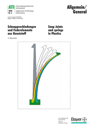
  • 4. 4 1 Grundsätzliches 1.1 Allgemeine Beschreibung Schnappverbindungen stellen eine einfache und kostengünstige Art der Verbindungstechnik dar. Sie sind charakteristisch für die Werkstoffgruppe der Kunststoffe, da deren Werkstoffeigen- schaften (Flexibilität) und Formgebungsmöglichkeiten ihrer Realisierung besonders entgegen kommen. Grundsätzlich sind Schnappverbindungen aus einem elastischen Federelement und einer Rastvorrichtung (Hinterschnitt) aufge- baut. Ihre Funktion teilt sich in den Füge- bzw. Löse- sowie den Haltevorgang. 1.2 Ausführungsarten Die Schnappverbindungen werden nach der Art des Feder- elements und nach der Lösbarkeit der Verbindung eingeteilt. Es wird grundsätzlich zwischen a) den Schnapparmverbindungen (Biegebalkenprinzip), b) den Torsionsschnappverbindungen (Torsionsstabprinzip), c) den Ringschnappverbindungen (zylindrische Profile) und d) den ringartigen Schnappverbindungen (regelmäßige Polygonprofile) unterschieden. In Abb. 1 sind diese vier Prinzipien schematisch dargestellt. 1. Basic information 1.1 General description Snap joints are a simple and inexpensive joining technique. They are a characteristic type of joint used for polymer materials, since the material properties (flexibility) and moulding poten- tial of polymers are particularly conducive to this kind of connection. Snap joints are essentially made up of an elastic spring element and a click-stop device (undercut). They serve the purpose of joining or separating parts and holding them together. 1.2 Types of snap joint Snap joints are classified according to the type of spring element and the separability of the joint. A basic distinction is drawn between a) the snap arm joint (flexural beam principle) b) the torsional snap joint (torsion rod principle) c) the annular snap joint (cylindrical profiles) d) the ring-shaped snap joint (regular polygon profiles) These four principles are shown in diagram form in Fig. 1. Fig. 1: Types of snap jointAbb. 1: Schnappverbindungsarten a) b) c) d)
  • 5. 5 In Abhängigkeit vom Hinterschnittwinkel wird außerdem noch zwischen lösbaren und unlösbaren Schnappverbindungen unter- schieden (Abb. 2). A distinction is also made between separable and inseparable joints, as a function of the undercut angle (Fig. 2). Fig. 2: Separable and inseparable jointAbb. 2: Lösbare und unlösbare Schnappverbindungen 1.3 Allgemeine Auslegungshinweise Die Auslegung einer Schnappverbindung beinhaltet eine opti- male Abstimmung der Konstruktion auf den Werkstoff. Hierzu ist die genaue Kenntnis der Belastungsverhältnisse und der Werkstoffeigenschaften erforderlich. 1.3.1 Belastungsverhältnisse Die Belastungsverhältnisse einer Schnappverbindung unter- scheiden sich grundlegend in Abhängigkeit von der Funktion. Während der Fügevorgang in der Regel eine einmalige oder mehrmalige kurzzeitige Belastung darstellt, bei der der Werkstoff relativ hoch beansprucht werden darf, wird die Haltefunktion meist von einer statischen Langzeit- oder gar Dauerbelastung bestimmt, die eine deutlich geringere maxi- male Beanspruchung zulässt. D. h., die Auslegung muss sowohl den Füge- bzw. Löse- als auch den Haltevorgang umfassen. 1.3.2 Beanspruchung Bei der Auslegung darf nicht vergessen werden, dass die Belas- tung sowohl beim Füge- als auch beim Haltevorgang meist zu mehreren überlagerten Lastfällen führt (z.B. Zug-, Scher- und Biegebelastung), die in ihrer Wechselwirkung (Vergleichsspan- nung bzw. -dehnung) berücksichtigt werden müssen. Ab einem Verhältnis der Schnapparmlänge zu seiner Höhe von kleiner als 5, sollte der Anteil der Schubverformung nicht unberücksichtigt bleiben. 1.3 General design advice The layout of a snap joint involves optimally tailoring the design to the material. This requires precise knowledge of the loading conditions and the material properties. 1.3.1 Loading conditions The loading conditions for a snap joint differ fundamentally as a function of the purpose that the snap joint serves. While the joining operation generally imposes once-only or repeated short- term load, during which time the material can be subjected to a relatively high load level, the retaining function generally involves a static long-term or even permanent load, where the maximum permitted load is considerably lower. In other words, the layout must be based on the joining and separation operation as well as on the retaining function. 1.3.2 Loading When conducting the layout, it must be remembered that both the joining and the retaining operation generally involve a number of different load cases being superimposed on each other (e.g. tensile, shear and flexural load), and it is necessary to make allowance for the interaction of these loads (effective stress, effective strain). Where the ratio of the snap arm length to the snap arm height is smaller than 5, consideration must also be paid to the shear deformation component.
  • 6. 6 1.3.3 Relaxation – retardation In order to make allowance for the time-dependent behaviour of the mechanical properties of plastics, it is important to achieve a stress-free and positive-action connection as far as possible (a form-fit rather than a friction-lock joint). If this is not entirely possible, then allowance can be made for – relaxation: stress falls over time with constant strain or – retardation: strain increases over time with constant stress with the aid of isochronous stress-strain curves. Information on this is shown in graphic form in Fig. 4. 1.3.3 Relaxation – Retardation Um dem zeitabhängigen Verhalten der mechanischen Eigen- schaften von Kunststoffen Rechnung zu tragen, sollte nach dem Einrasten eine möglichst entspannte und formschlüssige Ver- bindung (Formschluss vor Kraftschluss) angestrebt werden. Ist dies nicht vollständig möglich, so kann – die Relaxation: Spannung fällt bei konstanter Dehnung mit der Zeit ab oder – die Retardation: Dehnung nimmt bei konstanter Spannung mit der Zeit zu anhand von isochronen Spannungs-Dehnungs-Kurven berück- sichtigt werden. In Abb. 4 sind entsprechende Hinweise hierzu graphisch dargestellt. Biegespannung / Bending stress: σb = Mb W = Zugspannung / Tensile stress: σz = F A = F b · h = 0.5 · F h2 z Scherspannung / Shear stress: τs = F A = F a · b = 0.42 · F h2 s σb ÷ 6 ÷ 1 ÷ 0.84σz τs÷ = Schlussfolgerung: Biegebeanspruchung ist meist die dominierende Beanspruchungsart. Conclusion: Bending stress is mostly the dominant stress type. Beispiel der Beanspruchung eines Schnapparms durch die Haltekraft (FH)/ Example of the stress status of a cantilever arm by cohesion (FH) a = 1.2 · h, b = 2 · h, lm = h F · l b · h m 2 = 3 · F h2 6 · Abb. 3: Zusammengesetzte Beanspruchung Fig. 3: The combined loads that act h b a lm neutrale faser neutral fibre FH
  • 7. 7 1.3.4 Kerbwirkung Ein nach wie vor relativ häufiger Konstruktionsfehler betrifft die Kerbwirkung. Besonders deutlich macht sich dieser Fehler bei amorphen Werkstoffen bemerkbar. Aus diesem Grund wird hier ausdrücklich auf die Notwendigkeit der Abrundung von Ecken und Kanten bzw. der Vermeidung von Gratbildung in den beanspruchten Bereichen hingewiesen. Als günstig hat sich in der Praxis ein Kerbradius von 0,5 mm erwiesen. In Abb. 5 ist der Zusammenhang zwischen dem Kerbradius und der Spannung exemplarisch dargestellt. 1.4 Verteilung der Auslenkung auf die Fügepartner Im ungünstigsten Fall muss einer der beiden Fügepartner um den Gesamtbetrag der Auslenkung (Hinterschnitt) verformt werden. Tatsächlich verteilt sich die Verformung in der Regel auf beide Fügepartner. Die Verformungsverteilung auf die Fügepartner kann am ein- fachsten graphisch ermittelt werden. Hierzu muss für jeden der beiden Fügepartner zuerst ein Kraft-Verformungs-Diagramm (Federkennlinie), wie in Abb. 6 dargestellt, bestimmt werden. Die Überlagerung beider Federkennlinien ergibt einen Schnitt- punkt, der die tatsächliche Auslenkkraft und die Verformungs- anteile beider Fügepartner angibt. 1.3.4 Notch effect One design error still committed fairly frequently relates to the notch effect. This error is particularly noticeable with amor- phous materials. For this reason, the importance of rounding corners and edges and avoiding flash in areas subject to load must be stressed here. A notch radius of 0.5 mm has proved favourable in practice. Figure 5 shows the correlation between the notch radius and the stress on the basis of an example. 1.4 Dividing up the deflection over the mating parts In the least favourable case, one of the two mating parts needs to be deformed by the full amount of the deflection (undercut). As a rule, however, the deformation will be divided over both the mating parts. The easiest way to establish the distribution of the deformation over the mating parts is on a graph. To do this, it is first necess- ary for a force-deformation diagram (spring characteristic) to be established for each of the two mating parts, as shown in Fig. 6. By superimposing the two spring characteristics, a point of intersection is obtained which indicates the actual deflection force and the deformation components of the two mating parts. Abb. 4: Relaxation und Retardation (Kriechen) Fig. 4: Relaxation and retardation (creep)
  • 8. 8 Abb. 5: Spannung in Abhängigkeit vom Kerbradius bei gleicher Verformung Fig. 5: Stress versus the notch radius for identical deformation Bei Torsionsschnappverbindungen setzt sich die Gesamtver- formung des Torsionsarms aus der Drillverformung und aus der Biegeverformung zusammen. Oft kann der Anteil der Biege- verformung zwar vernachlässigt, er soll jedoch nicht vergessen werden. Abgesehen davon, muss die Biegeverformung des Betätigungshebels bei der Auslegung des Betätigungsweges (Anschlag) berücksichtigt werden. Für die Ringschnappverbindungen sind entsprechende Feder- kennlinien in Abb. 28 dargestellt. Hierbei wird davon ausge- gangen, dass wegen der Zugbeanspruchung bzw. der Dehnung (= versagensrelevante Größe) die Nabe der auszulegende Füge- partner ist und die Gesamtverformung (Hinterschnitt) aufzu- nehmen hat (Nabe flexibel – Welle starr). Trifft dies nicht zu, ist die tatsächliche Werkstoffbeanspruchung entsprechend gerin- ger. Bei gleich steifen Fügepartnern halbiert sich die Beanspru- chung, d. h., der zulässige Hinterschnitt ist doppelt so groß wie bei starr angenommener Welle. 1.5 Zulässige Auslenkung Die zulässige Auslenkung f (zulässiger Hinterschnitt) kann in Abhängigkeit von der zulässigen Dehnung des verwendeten Werkstoffs berechnet werden. Sie soll weder beim Einschnapp- vorgang noch bei der gewaltsamen Entformung aus dem Spritz- gießwerkzeug (Temperatur!) überschritten werden. In the case of torsional snap joints, the overall deformation of the torsion arm is made up of the twisting deformation and the flexural deformation. In many cases it is possible to neglect the flexural deformation component, but it should not be forgotten. Apart from this, allowance must be made for the flexural defor- mation of the actuating arm when designing the actuating path (catch). Corresponding spring characteristics are set out in Fig. 28 for annular snap joints. It is assumed here, on the basis of the tensile stressing or strain (= parameter of relevance for failure), that the hub is the mating part that is to be designed and this has to absorb the overall deformation (undercut), i.e. the hub is flexible and the shaft rigid. If this is not the case, the actual load acting on the material will be correspondingly smaller. With mating parts of identical rigidity, the load is halved, in other words, the permitted undercut is twice as big as for a shaft assumed to be rigid. 1.5 Permitted deflection The permitted deflection f (permitted undercut) can be calcu- lated as a function of the permitted strain of the material being used. This should not be exceeded during the snap-in opera- tion or during removal from the injection mould (attention to be paid to the temperature).
  • 9. 9 1.5.1 Zulässige Dehnung Beim Fehlen genauer Angaben kann die zulässige Dehnung oder Spannung bei einer einmaligen kurzzeitigen Auslenkung bei 23 °C anhand der folgenden Regel abgeschätzt werden: q nahezu die Streckdehnung bei teilkristallinen Thermoplasten q ca. 70% der Streckdehnung bei amorphen Thermoplasten q ca. 50 % der Bruchdehnung bei glasfaserverstärkten Thermo- plasten In Abb. 7 ist dieser Zusammenhang graphisch dargestellt. 1.5.1 Permitted strain If precise data is not available, the permitted strain or stress for a brief, once-only deflection at 23 °C can be estimated by using the following rule: q almost the tensile strain at yield for semi-crystalline thermo- plastics q approx. 70% of the tensile strain at yield for amorphous thermoplastics q approx. 50% of the tensile strain at break for glass-fibre rein- forced thermoplastics This relationship is depicted in graph form in Fig. 7. Abb. 6: Verteilung der Auslenkung auf die Fügepartner Abb. 7: Bestimmung der zulässigen Dehnung für den Einschnappvorgang (links: Werkstoff mit aus- geprägter Streckgrenze; rechts: glasfaserver- stärkter Werkstoff ohne Streckgrenze) Fig. 7: Determination of the permitted strain for the snap-in operation (left: material with a distinct yield point; right: glass fibre reinforced material without a yield point) Fig. 6: Distribution of the deflection of the mating parts a) Fügepartner / Mating part 1 Federweg / Deflection 0 1/3f 2/3f f Querkraft/TransverseforceQ b) Fügepartner / Mating part 2 01/3f2/3ff Querkraft/TransverseforceQ c) Fügepartner / Mating parts 1 + 2 gesamter Federweg f = Hinterschnitt / total deflection f = untercut tatsächl. Auslenkkraft/ realdeflection forceQ Federweg/ Deflection f1 Federweg/ Deflection f2 =+ Federweg / Deflection Spannung/Stressσ Dehnung / Strain ε 0.7 x εs εs Spannung/Stressσ Dehnung / Strain ε 0.5 x εB εB amorph / amorphous teilkristallin / semi-crystalline GF-Produkte / GRP products
  • 10. 10 Für einige Werkstoffe sind die zulässigen Dehnungen für eine einmalige kurzzeitige Belastung als Richtwerte (in %) in Tab. 1 aufgeführt: Table 1 shows the permitted strains for brief, once-only loading for a number of materials. These values are guide values, given in percent. teilkristallin / amorph / glasfaserverstärkt / semi-crystalline amorphous glass fibre reinforced PE 8% PC 4% PA 6-GF~ 2.0% PP 6% (PC+ABS) 3% PA 6-GF^ 1.5% PA ~ 6% ABS 2.5% PC-GF 1.8% PA ^ 4% CAB 2.5% PBTP-GF 1.5% POM 6% PVC 2% ABS-GF 1.2% PBTP 5% PS 1.8% ~ : konditioniert / conditioned, ^ : spritzfrisch / as moulded Bei häufiger kurzzeitiger Betätigung kann in etwa von ca. 60 % der einmalig zulässigen Werte ausgegangen werden. Bei Langzeit- oder Dauerbelastung besteht bei amorphen Pro- dukten die Gefahr der Spannungsrissbildung. Sie muss geson- dert berücksichtigt werden. Untersuchungen haben gezeigt, dass bei Dehnungen unterhalb ca. 0,5 % die Spannungsrissgefahr (bei 23 °C in Luft) deutlich geringer ist. Eine differenziertere Abschätzung von zulässigen Bemes- sungskennwerten vieler Bayer-Thermoplaste unter Berücksich- tigung der Belastungsdauer, der Temperatur, der Belastungsart, der Orientierung, der Bindenaht usw. erlaubt das Programm „RALPH“ , das unter der folgenden Adresse angefordert werden kann: Bayer-AG, KU-EU/INFO, Geb. B 207, 51368 Leverkusen. 1.5.2 Zulässige Torsionsspannung Bei Torsionsbelastung entsteht Schubbeanspruchung. Die zuläs- sige Torsionsschubspannung τzul kann für die meisten Kunst- stoffe überschlägig nach der folgenden Beziehung abgeschätzt werden: With frequent brief actuation, it is possible to work on the basis of approx. 60 % of the permitted values for once-only actuation. With long-term or permanent load, there is a danger of stress cracking with amorphous products. Extra allowance must be made for this. Studies have shown that the danger of stress cracking (at 23 °C in air) is considerably lower with a strain of less than around 0.5 %. The “RALPH” program permits a differentiated estimate of permitted dimensioning values for a large number of Bayer thermoplastics, making allowance for the loading duration, the temperature, the nature of the loading, the orientation and the weld line, etc. This program may be ordered from: Bayer-AG, KU-EU/INFO, Geb. B 207, D-51368 Leverkusen. 1.5.2 Permitted torsional stress Shear stressing results under torsional load. The permitted torsional shear stress τzul can be estimated on an approximate basis for the majority of plastics with the following relationship: Tab. 1: Richtwerte für zulässige Dehnungen bei einmaliger kurzzeitiger Belastung Table 1: Guide values for permitted strains for brief, once-only loading
  • 11. 11 Die Querkontraktionszahlen „ν“ (= Poisson-Zahlen) liegen bei gängigen Thermoplasten im Bereich von ca. 0,33 – 0,45. Der untere Wert gilt hierbei für hoch glasfaserverstärkte und der obere für hoch elastomermodifizierte Thermoplaste. Beim Fehlen genauer Angaben wird oft ein Wert von 0,35 benutzt. Mit der linearen Mischungsregel kann für den zeit- und tempe- raturabhängigen Sekantenmodul ES eine entsprechende Quer- kontraktionszahl bestimmt werden. The Poisson's ratios “ν” are between some 0.33 and 0.45 for commonly-used thermoplastics. The lower value here applies for thermoplastics with a high level of glass fibre reinforcement and the upper value for highly elastomer-modified thermoplastics. If a precise figure is not available, a value of 0.35 is frequently used. Applying the linear mixing rule, it is possible to determine an appropriate Poisson's ratio for the time and temperature- dependent secant modulus, ES. Abb. 8: Ermittlung des Sekanten-Moduls Fig. 8: Determination of the secant modulus Spannung/Stressσ Dehnung / Strain ε E0 εl Sekanten-Modul / Secant modulus ES ES = σl ε1 σl 1.6 Auslenkkraft Die Auslenkkraft kann in Abhängigkeit von der geometrischen Steifigkeit (Querschnittgestaltung), der zulässigen Dehnung und der Werkstoffsteifigkeit (E-Modul) entsprechenden berechnet werden. Da die beim Fügevorgang auftretenden Dehnungen oft außer- halb des Proportionalitäsbereichs der Spannungs-Dehnungs- Kurve liegen, sollte der Genauigkeit wegen, anstatt des Elasti- zitätsmoduls der sogenannte „Sekanten-Modul“ (= dehnungs- abhängiger Elastizitätsmodul) für die Bestimmung der Aus- lenkkraft verwendet werden. Seine Ermittlung ist in Abb. 8 dar- gestellt. Hierbei ist immer jene Dehnung einzusetzen, die für die erforderliche Auslenkung ermittelt wurde. Für einige Bayer-Thermoplaste ist der Sekanten-Modul in Abhängigkeit von der Dehnung in Abb. 9 dargestellt. 1.6 Deflection force The deflection force can be calculated as a function of the geo- metrical rigidity (cross-sectional shape), the permitted strain, and the rigidity of the material (Young’s modulus). Since the strains that occur during the joining operation are fre- quently outside the proportionality range of the stress-strain curve, the so-called “secant modulus” (= strain-dependent Young’s modulus) should be used instead of the Young's modu- lus, since this will allow the deflection force to be determined more accurately. Figure 8 shows how this is established. The strain determined for the requisite deflection must always be entered here. The secant modulus for a number of Bayer thermoplastics is shown in Fig. 9 as a function of strain.
  • 12. 12 Abb. 9: Sekantenmoduli einiger Bayer-Thermoplaste Fig. 9: Secant moduli of a number of Bayer thermo- plastics 16000 MPa 12000 10000 8000 6000 4000 2000 0 0 0,5 11 1,5 2 2,5 3 % 4 Dehnung / Strain Sekantenmodul/Secantmodulus Durethan B BKV 50 H1.0 ^ BKV 30 H1.0 ^ BKV 50 H1.0 ~ BKV 15 H1.0 ~ B 30 S ~ B 30 S ^ BKV 30 H1.0 ~ BKV 15 H1.0 ^ ^ = spritzfrisch ~ = konditioniert * Versuchsprodukt s. Prospektrückseite ^ = as moulded ~ = conditioned * Trial product see back page
  • 13. 13 1.7 Fügekraft Bei der Montage müssen die Auslenkkraft Q und die Reibungs- kraft R überwunden werden (Abb. 10). Die Fügekraft F ergibt sich aus: Bei lösbaren Verbindungen kann analog der Fügekraft auch die Lösekraft bestimmt werden. In diesem Fall ist der Neigungs- winkel der Löseflanke α’ in die obige Gleichung einzusetzen. Bedingt durch die stark schwankenden Reibungsverhältnisse, können die Fügekräfte in der Regel nur mit einer entsprechend großen Toleranz abgeschätzt werden. 1.7 Mating force When the parts are joined, the deflection force Q and the fric- tion force R have to be overcome (Fig. 10). The mating force F is obtained from With separable joints, the separation force can be determined in the same way as the mating force. In this case, the angle of inclination to be introduced into the above equation is the angle of the separation side, α’. The highly fluctuating friction conditions mean that the mating forces can generally only be estimated with a correspondingly high tolerance. Abb. 10: Zusammenhang Auslenkkraft – Fügekraft Tab. 2: Richtwerte für Gleitreibungskoeffizienten Table 2: Guide values for coefficients of sliding friction 1.8 Reibungskoeffizienten In Tab. 2 sind einige Anhaltswerte für Gleitreibungskoeffizi- enten für die Reibpaarung Kunststoff – Stahl aufgeführt. Sie sind der Literatur entnommen. Bei einer Paarung Kunststoff - anderer Kunststoff kann (nach VDI 2541) mit gleichen oder etwas niedrigeren Werten gerechnet werden, wie in der unteren Tabelle angegeben. Bei gleichen Reibungspartnern ist meist mit höheren Reibungskoeffizienten zu rechnen. Soweit bekannt, sind die entsprechenden Werte in Tab. 2 angegeben. Fig. 10: Relationship between deflection force and mating force 1.8 Coefficients of friction Table 2 shows a number of guide values for the coefficients of sliding friction for the friction combination of plastic and steel. These have been taken from the literature. Where a plastic is combined with a dissimilar plastic, it is possible to use the same or slightly lower values, according to VDI 2541, as is shown in the Table below. Where the two parts are made of the same material, then higher coefficients of friction must generally be expected. The corresponding values are given in Table 2 insofar as they are known. Reibungskoeffizienten / Coefficients of friction Werkstoff / Kunststoff – Stahl / Gleiche Reibungspartner / Material Plastic – Steel Identical friction partners PTFE 0.12 – 0.22 0.12 – 0.22 PE-HD 0.20 – 0.25 0.40 – 0.50 PP 0.25 – 0.30 0.38 – 0.45 POM 0.20 – 0.35 0.30 – 0.53 PA 0.30 – 0.40 0.45 – 0.60 PBTP 0.35 – 0.40 – PS 0.40 – 0.50 0.48 – 0.60 SAN 0.45 – 0.55 – PC 0.45 – 0.55 0.54 – 0.66 PMMA 0.50 – 0.60 0.60 – 0.72 ABS 0.50 – 0.65 0.60 – 0.78 PE-LD 0.55 – 0.60 0.66 – 0.72 PVC 0.55 – 0.60 0.55 – 0.60
  • 14. 14 Abgesehen davon sind die Reibungskoeffizienten abhängig von der Gleitgeschwindigkeit, dem Anpressdruck und der Ober- flächenbeschaffenheit, was durch eine entsprechende Toleranz berücksichtigt werden sollte. 1.9 Gestaltung: Um möglichst große Hinterschnitte (= Fügesicherheit) reali- sieren zu können, bedarf es optimaler Formgestaltung. Sie bein- haltet hauptsächlich die Wahl der Querschnittsform und des Querschnittsverlaufs des Federelements. Die Querschnittsform wird durch die maßgebliche Belastungs- art (beim Füge- oder Haltevorgang) bestimmt. Als optimal sind hierbei folgende Querschnittsformen und Ausführungen anzu- sehen: q Zugbelastung ³ konstanter Rechteckquerschnitt (s. Abb. 13, Ausführung 1) q Biegebelastung ³ verjüngter Rechteckquerschnitt (s. Abb. 13, Ausführung 2 oder 3) q Torsionsbelastung ³ konstanter Kreisquerschnitt Das Optimum kann u. U. erst durch eine Kombination der o.g. Querschnittsformen und/oder ihrer Ausführungsarten erreicht werden. Alle anderen Querschnittsformen und -verläufe stellen Kom- promisslösungen dar. Die Wahl des optimalen Querschnitts kann neben den mechanischen Aspekten auch z. B. durch fließtech- nische (Fließweg) Belange mitbestimmt werden. In addition to this, the coefficients of friction are conditioned by the sliding velocity, the contact pressure and the surface finish. Allowance should be made for this through the corresponding tolerance. 1.9 Design advice In order to achieve the biggest possible undercuts (= secure joint), it is essential to ensure the optimum design. This essen- tially involves selecting the cross-sectional shape and the cross- sectional profile of the spring element. The cross-sectional shape is determined by the decisive load type (during the mating or retaining operation). The optimum cross-sectional shapes and designs are as follows: q tensile load ³ constant square cross-section (see Fig. 13, design type 1) q flexural load ³ tapered square cross-section (see Fig. 13, design type 2 or 3) q torsional load ³ constant circular cross-section In certain cases, the optimum design can only be achieved by combining the above cross-sectional shapes and/or design types. All other cross-sectional shapes and profiles are compromise solutions. The selection of the optimum cross-section can also be conditioned not only by mechanical aspects but also by flow considerations (flow path).
  • 15. 15 2. Schnapparmverbindungen 2.1 Berechnungsgrundlagen 2. Cantilever snap arm joints 2.1 Design and calculation criteria Geometriefaktor „x“ siehe Abb. 13 Widerstandsmomente „W“ siehe Abb. 13 und 15 Die Dehnung „ε“ ist als Absolutwert einzusetzen Geometry factor “x”, see Fig. 13 Moments of resistance “W”, see Figs. 13 and 15 Strain “ε” is to be entered as an absolute value h fQl F Abb. 11: Prinzipdarstellung Abb.12: Dimensionen Auslenkung: (s. Abb. 13) Deflection: (see Fig. 13) Auslenkkraft: (s. Abb. 13 und 15) Deflection force: (see Figs. 13 and 15) Fügekraft: (s. Abb. 10) Mating force: (see Fig. 10) Fig. 11: Basic principle Fig. 12: Dimensions
  • 16. 16 6DieSchnapparmesindimmerbezüglichdermaximalenZugbeanspru- chung(Versagenskriterium)auszulegen.Deshalbsindimmerdiejenigen Randfaserabstände„e“undWiderstandsmomente„W“zubetrachten, diesichaufdiezugbeanspruchteRandfaserbeziehen.BeimTrapez- querschnitt(B)sindggf.aundbzuvertauschen. 66DieGeometriefaktoren„C“fürKreisringsegmente(s.Abb.13)sindin Abb.14graphischdargestellt. 6Thecantileversnaparmsmustalwaysbedesignedtocopewiththe maximumtensileload(failurecriterion).Itisthusimportanttoalways observetheouterfibrespacing“e”andmomentsofresistance“W”that relatetotheouterfibrethatissubjecttotensilestressing.Forthetrape- zoidalcross-section(B),aandbshouldbeexchangedifnecessary. 66Geometryfactors“C”forcircularringsegments(seeFig.13)areshown onthegraphsinFig.14. b a h r ϕ 2 h b e e h b 1 2 3 (zulässige)Auslenkung (permissible)Deflection Auslenk-Kraft Deflec.force Querschnittsform / Shape of cross section Ausführung / Type of design Rechteck / RectangleA: Trapez / TrapeziumB: Ringsegment / Ring segmentC: beliebig / irregularD: =f 0.67 · h0 ε · l2 =f 0.82 · h0 ε · l2 =f 1.20 · h0 ε · l2 =f · h0 ε· l2 2a+b a+b6 = 1.79f · h0 ε· l2 2a+b a+b6 =1.22f · h ε· l2 2a+b a+b6 W6 l Es · ε · =Q · 2a+b a2 + 4ab+ b2 12 h0 2 = C66f r2 ε· l2 = 1.79 · C66f r2 ε· l2 = 1.22 · C66f r2 ε· l2 =Q 6 bh0 2 · l Es · ε W6 { · =Q W6 · l Es · ε f e6 ε· l2 = 3 1 · f e6 ε· l2 = 0.60· f e6 ε· l2 = 0.41· =Q W6 · l Es · ε e2 e1 e2 e1 e2 e1 r∇ r1 h1:h0 =1:1 b1:b0 =1:1 h1 b1 b0 h0 1 h1:h0 =1:2.5 b1:b0 =1:1.0 h1 b1 b0 h0 1 h1:h0 =1:1 b1:b0 =1:4 h1 b1 b0 h0 1 Abb.13:BerechnungsgleichungenfürSchnapparmeFig.13:Equationsfordimensioningofcantileversnap arms
  • 17. 17 Abb.16+17: Widerstandsmoment für Kreisring- segmente Fig.16+17: Moment of resistance for circular ring segments W1: Konkavseite unter Zugspannung / Concave side under tension W2: Konvexseite unter Zugspannung / Convex side under tension ϕ in° 180 165 150 135 120 105 90 75 60 45 30 15 r2 3 r2 3 W2 W2 .= 1 2 4 6 8 10 20 40 60 80 100 200 400 600 800 1000 10 6 4 2 10 6 4 2 6 4 −1 −2 −3 −4 2 10 10 W2/r2 3 4 6 8 10 20 40 60 80 100 1 2 r2 0,50 0,60 0,70 0,80 0,90 1,00 ϕ in° 180 165 150 135 120 105 90 75 60 45 30 15 r2 3 r2 3 W1 W1 .= Beispiel: r1 = 8,75 r2 = 10 ϕ = 75° 3,9 1 2 4 6 8 10 20 40 60 80 100 200 400 600 800 1000 4 6 8 10 20 40 60 80 100 1 2 r2 2 10 6 4 2 10 6 4 2 6 4 −1 −2 −3 −4 2 10 10 W1/ρ2 3 0,50 0,60 0,70 0,80 0,90 0,875r1/r2 1,00 r1/r2 Abb.14+15: Geometriefaktoren „C“ für Kreisring- segmente Fig.14+15: Geometry factors “C” for circular ring segments 10 8 6 4 2 100 8 6 1 0,5 0,6 0,7 0,8 0,9 1,0 15 30 45 60 75 90 105 120 135 150 165 180 10 8 6 4 2 100 8 6 1 0,5 0,6 0,7 0,8 0,9 1,0 30 45 60 75 90 105 120 135 150 165 180 2,67 0,875 ϕ in° 15 C1: Konkavseite unter Zugspannung / Concave side under tension C2: Konvexseite unter Zugspannung / Convex side under tension C2C1 ϕ in° r1/r2 r1/r2
  • 18. 18 Abb.18: Spannungsverteilung in Abhängigkeit von der Querschnittsgestaltung bei gleicher Verformung Fig. 18: Stress distribution versus cross-section design for constant deformation
  • 19. 19 2.2 Berechnungsbeispiel eines Schnapparms 2.2 Calculation example for a cantilever snap arm Abb.19: Abmessungen Anwendung: Der Schnapparm soll zwei Gehäusehälften miteinander verbin- den, wobei er im montierten Zustand eine minimale Auslenkung zu ertragen hat. Ausführung: Aus der Anwendung geht hervor, dass die Ausführung 2 (s. Abb. 13) hier als die optimale anzusehen ist. Werkstoffdaten: Type: Novodur P2H-AT (ABS) Sekanten-Modul: Es = 2400 MPa (ε = 1,25%) zul. Dehnung: εz = 2,5% (s. 1.5 Abb. 7) Gegeben: Querschnittsform: A (= Rechteck) Länge: l = 20 mm Breite: b = 10 mm (konstant) Hinterschnitt: f = 2,2 mm Schrägungswinkel: α = 30° Reibungskoeffizient: -- µ = 0,60 – 0,78 = 0,69 Gesucht: – Querschnittsdicke h0, bei der bei voller Auslenkung die Hälfte der zulässigen Dehnung (= 1,25%) erreicht wird – Auslenkkraft Q – Montagekraft F Lösung: – Ermittlung der Querschnittsdicke h0 Geforderte Dehnung = 0,5 · 2,5% = 1,25% = 0,0125 Gewählte Ausführung: 2 Fig.19: Dimensions Application: The cantilever snap arm is to be used to join two halves of a housing. It will be subject to a minimal level of deflection in the assembled state. Design: On the basis of the application, design type 2 would appear to be the optimum design in this case (see Fig. 13). Material data: Type: Novodur P2H-AT (ABS) Secant modulus: Es = 2400 MPa (ε = 1.25%) Permitted strain: εz = 2.5% (see 1.5, Fig. 7) Given: Cross-sectional shape: A (= square) Length: l = 20 mm Width: b = 10 mm (constant) Undercut: f = 2.2 mm Angle of inclination: α = 30° Coefficient of friction: -- µ = 0.60 – 0.78 = 0.69 Unknown: – cross-sectional thickness h0 at which half the permitted strain (= 1.25%) is attained at full deflection. – deflection force Q – assembly force F Solution: – establishment of the cross-sectional thickness h0 Requisite strain = 0.5 · 2.5% = 1.25% = 0.0125 Selected design type: 2 Schema:
  • 20. 20 Aus der Durchbiegungsgleichung für ein Rechteckprofil folgt: – Ermittlung der Auslenkkraft Q (Abb. 13) – Ermittlung der Fügekraft F (s. 1.7, Abb. 10) FEM-Ergebnisse: Die Nachrechnung dieses Beispiels mittels der FE-Methode ergab für die o. g. Abmessungen (s. Abb. 19) eine maximale Dehnung von 1,23% (s. Abb. 20) und eine Auslenkkraft von 18 N. From the deflection equation for a square profile, it follows that: – establishment of the deflection force Q (Fig. 13) – establishment of the mating force F (see 1.7, Fig. 10) FEM results: When this example was recalculated by the finite element method for the above dimensions (see Fig. 19), a maximum strain of 1.23% (see Fig. 20) and a deflec- tion force of 18 N was obtained. ε · l – µ· tan α µ+ tan α = 1.2 ·h0 l2 = 1.2 · f 0.0125 · 202 mm2 2.2 mm = 2.7 mmh0 =Q b · h2 · 6 10 mm · 2.72 mm2 6 Es · ε = l 2400 · 20 mm · mm2 · 0.0125 N =Q 18N =F 0.69 + tan 30° 1 – 0.69 · tan 30° =F 38N Q · = 17N · Abb.20: Dehnungsverteilung Fig.20: Strain distribution
  • 21. 21 2.3 Anwendungsbeispiele 2.3 Sample applications geschnappte Gelenke / snap articulations axiale Schnapp- verbindung / axial snap joints Raster / Catchesradiale Federung / radial spring suspension Beispiel 1: Gefederte Drehgelenke (quasi stufenlose Verstellung um zwei Achsen) Example 1: Sprung pivot joints (virtually infinitely- variable adjustment around two axes) Beispiel 2: Biaxiale Scheinwerferhalterung Example 2: Biaxial headlamp fastening Demontage / Disassembly Montage / Assembly Demontage / Disassembly Beispiel 3: Elektrostecker für Schienenmontage Example 3: Electric plug for rail mounting
  • 22. 22 Beispiel 4: Geschlitzte Ringschnappverbindung Example 4: Annular snap joint with slits Beispiel 5: Integrierte Tastenfedern einer Fernbedienung Example 5: Integrated keys for a remote control unit Feder / spring Beispiel 6: Schalterstößel für Computer Example 6: Push-rod switch for a computer Beispiel 7: Spreitzniet mit Sicherungsstift Example 7: Expanding rivet with safety pin
  • 23. 3.1 Design and calculation criteria Note: γ and ezul = absolute values! Poisson's ratio ν ≈ approx. 0.35 Geometry factors K and from Fig. 22 23 3. Torsionsschnappverbindungen 3. Torsion snap joints Abb.21: Prinzipdarstellung Fig.21: Basic principle 3.1 Berechnungsgrundlagen Auslenkwinkel / Deflection angle: Auslenkkraft / Deflection force: Fügekraft / Mating force: Anmerkung: γ und εzul = Absolutwerte ! Querkontraktionszahl ν ≈ 0,35 Geometriefaktoren K und aus Abb. 22 =β K · a γ · l mit / where sin β = f1 l1 γ ≈ (l + ν) · εzul (= Scherung / shear) = f2 l2 Q1/2 · l1/2 = G · γ · a3 · Wp a3 mit / where Es 2(l + ν) G = Es 2.7 ≈(·2)1) F = Q1/2 · tan(α + ρ) mit / where µ = tan ρ Wp a3 Wp a3 1) nur wenn zwei Torsionsarme vorliegen (s. Abb. 23) 1) in case of two torsion arms (see Fig. 23)
  • 24. 24 Abb. 22: Konstanten zur Berechnung von Querschnittsdaten von Torsionsstäben 3.2 Berechnungsbeispiel einer Torsionsschnappverbindung Schema: Fig. 22: Constants for calculating the cross-sectional data of torsion rods 3.2 Calculation example for a torsion snap joint Diagram: l1 d f1 Q2 Einspannung Fixation Torsionsstab Torsion rod Einspannung Fixation l2 l ß Q1 f2 Abb. 23: Prinzipdarstellung Fig. 23: Basic principle K Wp a3 a b 1 1.5 2 3 4 6 8 10 84.8 67.0 61.9 58.4 57.8 57.5 57.3 57.3 0.354 0.494 0.808 1.130 1.790 2.460 3.1200.208 Torsionsarm- querschnitt / Cross-section for torsion arm K 57.3 132 84.8 1.57 0.05 0.208 a b 4 a 1 a a a 2 a a 3 Wp a3
  • 25. 25 Anwendung: Rastwippe Werkstoffdaten: Type Makrolon 2805 Sekanten-Modul: Es = 1500 MPa Schubmodul: G = 560 MPa zul. Dehnung: εz = 4 % (s. 1.5, Tab. 1) zul. Scherung: γz = 5,4 % Gegeben: Stabdurchmesser: d = 4 mm ergibt a = 2 mm Stablänge: l = 5 mm (zweifach vorhanden) Wippenlänge: l1 = 15 mm, l2 = 30 mm Hinterschnitt: f1 = 2,0 mm Gesucht: – auftretende Dehnung – Auslenkkraft Q Lösung: – Ermittlung der auftretenden Scherung (Dehnung) – Ermittlung der Auslenkkraft Q (s. 1.6, Abb. 8) – Ermittlung der Fügekraft F (s. 1.7, Abb. 10) Im vorliegenden Fall entspricht die Fügekraft der Auslenkkraft, da beide in die gleiche Richtung wirken. FEM-Ergebnisse: Eine Nachrechnung dieser Konstruktion mit Hilfe der FE-Methode ergab eine maximale Dehnung von ca. 3,8 % (s.Abb. 24) und eine Auslenkkraft von 21N. Application: Snap-fit rocker Material data: Type: Makrolon 2805 Secant modulus: Es = 1500 MPa Shear modulus: G = 560 MPa Permitted strain: εz = 4% (see 1.5, Tab. 1) Permitted shear: γz = 5.4 % Given: Rod diameter d = 4 mm, giving a = 2 mm l = 5 mm (occurs twice) Rocker length: l1 = 15 mm, l2 = 30 mm Undercut: fl = 2.0 mm Unknown: – prevailing strain – deflection force Q Solution: – determination of prevailing shear (strain) – determination of deflection force Q (see 1.6, Fig. 8) – determination of mating force F (see 1.7, Fig. 10) In the present case the mating force corres- ponds to the deflection force, since both act in the same direction FEM results: When this design was recalculated with the aid of finite element analysis, a maximum strain of around 3.8 % was obtained (see Fig. 24) and a deflection force of 21N. =γ β · a K · l sinβ = f1 l1 = 2.0 mm 15 mm = 0.133 =γ 7.7° · 2 mm 57.3 · 5 mm = 0.054 = 5.4% Q2 = G · γ · a3 · Wp a3 1 l2 · Q2 = 560 Wp a3 = 1.57 N mm2 · 0.054 · 23 mm3 · 1.57 · 1 30 mm Q2 = 25N · 2 · 2
  • 26. 26 f Dehnungsverteilung / Strain distribution Q Abb. 24: Dehnungsverteilung Fig. 24: Strain distribution
  • 27. 27 3.3 Anwendungsbeispiele: 3.3 Sample applications: Beispiel 1: Schriftblende, Airbus A 300 Makrolon® Example 1: Sign cover made of Makrolon® for the Airbus 300 Beispiel 2: Steckerblock Makrolon® Example 2: Connector block made of Makrolon®
  • 28. 28 4. Ringschnappverbindungen 4. Annular snap joints Schnappnut endnah / Snap groove close to the end f/2 d Q’ s dF F’ Q Schnappnut endfern / Snap groove remote from the end : δ > 1,8 d · s δ Abb. 25: Prinzipdarstellung 4.1 Berechnungsgrundlagen Abb. 26: Geometriedaten Die Berechnungsgleichungen beruhen auf der Annahme, dass sich einer der Fügepartner starr verhält. Bei gleichsteifen Fügepartnern kann der Hinterschnitt zur Hälf- te auf beide Partner verteilt werden. Die Verteilung der Aus- lenkung bei unterschiedlich steifen Fügepartnern ist unter 1.4 erläutert. Fig. 26: Geometrical data The calculation equations are based on the assumption that one of the mating parts is rigid. If both parts are of equal rigidity, then half the undercut can be incorporated on each of the parts. The distribution of the deflec- tion for parts of dissimilar rigidity is explained in section 1.4. Fig. 25: Basic principle 4.1 Design and calculation criteria
  • 29. 29 In Abhängigkeit von der Lage der Schnappnut, wird zwischen der endnahen und der endfernen Ringschnappverbindung unter- schieden. In der Regel liegt die Schnappnut endnah. Eine end- ferne Schnappnut liegt vor ab einem Abstand δ vom betrachte- ten Ende von A distinction is drawn between an annular snap joint close to the end and one remote from the end, as a function of the position of the snap groove. As a rule, the snap groove will be located close to the end. A groove counts as being remote from the end as of a distance δ from the end under observation of Auslenkung: f = ε · d ε = Absolutwert ! Dieser Zusammenhang stellt eine Vereinfachung dar, die eine konstante Dehnung über die gesamte Wanddicke annimmt, was nicht den Tatsachen entspricht (s. Abb. 27). Deflection: f = ε · d ε = absolute value! This relationship constitutes a simplification, assuming a constant strain over the entire wall thickness, which is not actually the case (see Fig. 27). Abb. 27: Spannungsverteilung beim Fügevorgang Auslenkkraft: Aufgrund der unterschiedlichen Beanspruchung muss bei der Abschätzung der Auslenkkräfte von Ringschnappverbindungen zwischen der endnahen und der endfernen Lage der Schnappnut unterschieden werden. Die Theorie hierzu ist [1] entnommen. Hiernach beträgt die Auslenkkraft bei der endfernen Schnapp- nut das Vierfache der endnahen. Praktische Untersuchungen haben jedoch gezeigt, dass die realen Fügekräfte sich kaum um den Faktor 3 unterscheiden. Deshalb wird hier für die endfer- ne Lage der Schnappnut der dreifache Wert der Auslenkkraft der endnahen Schnappnut zugrundegelegt. Fig. 27: Stress distribution during the joining operation Deflection force: In view of the dissimilar stressing that prevails, it is necessary to draw a distinction between a snap groove close to the end and one remote from the end when estimating the deflection forces of annular snap joints. The theory on this has been taken from [1]. This states that the deflection force for the snap groove remote from the end is four times that for a groove close to the end. Practical investigations, however, have shown that the actual mating force is only around three times greater. The mating force for a snap groove remote from the end is thus taken as being three times the value of the mating force for the snap groove close to the end. x Tangential-Spannung / Tangential stress σ S d F F’ Q Q’ δ
  • 30. 30 Der Geometriefaktor X kann Abb. 28 entnommen werden, wobei X = XN ist, wenn der äußere Fügepartner (Nabe) nachgiebig und der innere Partner (Welle) starr bzw. X = XW, wenn die Nabe starr und die Welle nachgiebig ist. Geometry factor X can be taken from Fig. 28, where X = XN if the outer mating part (hub) is flexible and the inner part (shaft) is rigid or X = XW if the hub is rigid and the shaft flexible. X X 1.00 1.04 1.08 1.12 1.16 1.20 0.04 0.03 0.02 0.01 0.00 XW XN XW XN 0.48 0.40 0.32 0.24 0.16 0.08 0.00 1.0 1.4 1.8 2.2 2.6 3.0 Welle nachgiebig, Narbe starr W N id d ad d Welle nachgiebig, Narbe starr Welle starr, Narbe nachgiebig / Shaft rigid, hub flexible ad d XN XW id d d/di (Welle / shaft) da /d (Narbe / hub) Shaft flexible, hub rigid Shaft flexible, hub rigid d/di (Welle / shaft) da /d (Narbe / hub) Welle starr, Narbe nachgiebig / Shaft rigid, hub flexible Abb. 28: Diagramme zur Bestimmung des Geometrie- faktors X für Ringschnappverbindungen Sie können auch nach den folgenden Formeln berechnet werden: Fügekraft: Fig. 28: Diagrams for determining geometry factor X for annular snap joints The factors can also be calculated with the following formulae: Mating force: XN = 0.62 · (da ÷ d – 1) ÷ (da ÷ d + 1) [(da ÷ d)2 + 1] ÷ [(da ÷ d)2 – 1] + ν nach / according to [1] XW = 0.62 · (d ÷ di – 1) ÷ (d ÷ di + 1) [(d ÷ di)2 + 1] ÷ [(d ÷ di)2 – 1] – ν nach / according to [1] =F Q · l – µ· tan α µ+ tan α mit / where µ = tan ρ (µ s. auch / see also 1.8)
  • 31. 31 4.2 Berechnungsbeispiel einer Ringschnappverbindung Schema: 4.2 Calculation example for an annular snap joint Diagram: =ε d f = 0.005 = 0.5% 200 mm 1 mm = Q = f · d · Es · X Einzelheit „X“ / Detail “X” ø 200 90° r2 90° „X“ f 2 Abb. 29: Objektdarstellung Anwendung: Leuchtenabdeckung und Gehäuse Ausführung: endnahe Schnappnut Werkstoffdaten: Type: Makrolon 2805 Sekanten-Modul: 2200 MPa zul. Dehnung: ca. 4% (siehe 1.5, Tab. 1) Gegeben: Durchmesser: d = 200 mm Wanddicke: s = 2,5 mm (bei beiden Fügepartnern) Hinterschnitt: f = 2 · 1 mm Schrägungswinkel: α = 30° Reibungskoeffizient: µ = 0,6 Gesucht: – auftretende Dehnung – Auslenkkraft Q – Fügekraft F Lösung: – Ermittlung der auftretenden Dehnung Da die Fügepartner in etwa gleich steif sind, wird davon ausgegangen, das sich der Hinterschnitt gleichmäßig auf beide verteilt. – Ermittlung der Auslenkkraft Q (s. 1.6, Abb. 8) Abb. 29: Diagram of the object Application: Lamp covers and housings Version: Snap ring close to end Material data: Type: Makrolon 2805 Secant modulus: 2200 MPa Permitted strain: approx. 4 % (see 1.5, Tab. 1) Given: Diameter: d = 200 mm Wall thickness: s = 2.5 mm (for both mating parts) Undercut: f = 2 · 1 mm Angle of inclination: α = 30° Coefficient of friction: µ = 0.6 Unknown: – prevailing strain – deflection force Q – mating force F Solution: – determination of the prevailing strain Since the mating parts are of roughly equal rigidity, it is assumed that the undercut is divided up uniformly over both parts. – determination of the deflection force Q (see 1.6, Fig. 8)
  • 32. 32 Bei gleicher Steifigkeit der Fügepartner ist es gleichgültig, für welchen der beiden die Berechnung durchgeführt wird. Hier wird sie für die äußere Lampenschale (= Nabe) durchgeführt. – Ermittlung der Fügekraft F (s. 1.7 Abb. 10) Der tatsächliche Schrägungswinkel beträgt 45°. Da die Kanten jedoch abgerundet sind, wird mit einem effektiven Schrä- gungswinkel von 30° gerechnet. Diese Fügekraft ist bei symmetrischem Fügen zu erwarten, was nur maschinell zu erreichen ist. Bei manuellem Fügen (asym- metrisch, stoßartig) kann die Fügekraft u. U. erheblich geringer sein. FEM-Ergebnisse: Eine FE-Analyse (siehe Abb. 30) der Beanspruchung dieses Pro- blems ergab im adäquaten Bereich eine vergleichbare Dehnung. Die maximale Dehnung (Randkante) liegt jedoch mit 0,65% etwas höher, da darin auch Randbiegeeffekte enthalten sind. If both mating parts are equally rigid, it does not matter which part is taken for the calculation. In this case, it is performed for the outer lamp shell (= hub). – determination of the mating force (see 1.7, Fig. 10) The actual angle of inclination is 45°. Since the edges are rounded, however, an effective angle of inclination of 30° is used for the calculation. This mating force can be expected when the joining operation is performed symmetrically – something that can only be achieved by mechanical means. When parts are joined manually (asym- metrically and with a jolt) the mating force can be considerably lower under certain circumstances. FEM results: An FE analysis (see Fig. 30) of the stressing involved in this problem showed a comparable strain in the appropriate zone. The maximum strain (outer edge) is somewhat higher at 0.65%, however, since edge bending effects are also contained in this. di da = 1.025 200 200 + (2 · 2.5) =XN = XN = 0.0017 · 0.0017 mm2 N Q = 1 mm · 200 mm · 2200 Q = 748N mit / where aus Abb. 28 / from Fig. 28 =F Q · l – µ· tan α µ+ tan α = 748N l – 0.6 · tan 30° 0.6 · tan 30° F = 1346N —.238E-03 .514E-03 .C01267 .C02019 .C02772 .C03525 .C04277 .C0503 .C05783 .C06535 f = 0.5 Modell rotationssymmetrisch / Axisymmetric model Abb. 30: Verteilung der Tangentialdehnung Fig. 30: Distribution of tangential strain
  • 33. 33 4.3 Anwendungsbeispiele: 4.3 Sample applications: Beispiel 1: Getriebegehäuse Example 1: Gearhousing Beispiel 2: Kleiderbügel mit drehbarem Haken Example 2: Coathanger with a rotatable hook
  • 34. 34 5. Ringartige Schnappverbindungen Die ringartigen Schnappverbindungen stellen Sonderformen der Ringschnappverbindung dar. Sie unterscheiden sich von dieser hauptsächlich dadurch, dass sie anstatt eines Kreisringquer- schnitts einen Polygonquerschnitt aufweisen. In diese Gruppe wurden aber auch geschlitzte Ringschnappverbindungen (siehe Schnapparme mit Kreisringquerschnitt, Abb. 13 Ausführung C) und Ringschnappverbindungen mit lokalen Hinterschnitten ein- bezogen. Solche Verbindungen werden vorzugsweise zur Verbindung von Behälterteilen eingesetzt. 5. Ring-shaped snap joints Ring-shaped snap joints are special types of annular snap joint. The main difference between ring-shaped and annular snap joints is that the former have a polygonal cross-section instead of a circular ring cross-section. This group, however, also takes in slotted annular snap joints (see cantilever snap arms with a circular ring cross-section, Fig. 13, Version C) and annular snap joints with local undercuts. Joints of this type are used primarily for connecting container components. Abb. 31: Prinzipdarstellung 5.1 Berechnungsgrundlagen Während es für die Abschätzung der Beanspruchung und der Auslenk- und Fügekräfte von Ringschnappverbindungen relativ einfache Berechnungshilfen gibt (siehe 4.1), ist eine Abschätzung dieser Größen bei den ringartigen Schnappver- bindungen nur mit Hilfe der FE-Methode möglich. Dieses Ver- fahren steht jedoch nicht jedem zur Verfügung. Deshalb wurde für einige ringartige Schnappverbindungen, anhand von FE- Berechnungen, eine einfache Abschätzhilfe erstellt. Sie erlaubt es durch eine einfache Analogiebetrachtung das Verhalten einer ringartigen Schnappverbindung anhand des Verhaltens einer adäquaten Ringschnappverbindung zu beurteilen. Die Auslenk- bzw. Fügekräfte und die zulässige Auslenkung sind darin in Relation zu den entsprechenden Größen einer adä- quaten Ringschnappverbindung in Form von Balkendiagram- men dargestellt. Innerhalb einer Polygonform wird der Einfluss der Anzahl und der Breite der lokalen Hinterschnitte und beim geteilten Kreisring die Tiefe der Schlitze berücksichtigt. Die Bezugsgröße stellt hierbei immer eine geschlossene Ring- schnappverbindung mit umlaufendem Hinterschnitt dar. Aus Abb. 32 kann der geometrischer Bezug zwischen der unter- suchten Polygonform und der adäquaten Kreisringgröße ent- nommen werden. Fig. 31: Basic principles 5.1 Design and calculation criteria While relatively simple calculation aids are available for estimating the stressing and the deflection and mating forces on annular snap joints (see 4.1), these parameters can only be estimated with the aid of the FE method for ring-shaped joints. Not everyone has access to this method, however. A simple estimation aid has thus been compiled for ring-shaped snap joints which is based on FE calculations. This makes it possible to assess the behaviour of a ring-shaped snap joint from the behaviour of an appropriate annular snap joint by means of a simple analogy observation. In this estimation aid, the deflection or mating forces and the permitted deflection are expressed in terms of the corresponding parameters for a corresponding annular snap joint and presented on a bar chart. The influence of the number and width of the local undercuts is taken into account for a polygon shape, and the depth of the slots taken into consideration for a divided circular ring. The reference system employed here is always a closed annular snap joint with a circumferential undercut. The geometrical relationship between the polygon shape investigated and the corresponding circular-ring size can be seen from Fig. 32. Patrize / Positive part Matrize / Negative part Kreisring / Circular ring Quadratischer Ring / Square ring Sechseckiger Ring / Hexagonal ring
  • 35. 35 Neben einem direkten Vergleich untereinander, kann anhand dieser Diagramme ebenso die Größenordnung der Kräfte und der zulässigen Auslenkung abgeschätzt werden. Dazu müssen ledig- lich die entsprechenden Größen einer adäquaten Ringschnapp- verbindung berechnet werden (s. 4.1) und mit dem zugehöri- gen Wert aus dem Diagramm (Absolutwert!) multipliziert werden. Apart from a direct comparison of the two systems, the order of magnitude of the forces and the permitted deflection can be estimated on the basis of these diagrams. All this requires is for the corresponding parameters of an appropriate annular snap connection to be calculated (see 4.1) and multiplied by the corresponding value from the diagram (absolute value!). Abb. 32: Größenbezug der einzelner Ringformen 0 = Kreisring = Bezugsgröße; 1 = Sechseck; 2 = Quadrat; 3 = Rechteck L/B = 1,5; 4 = Dreieck, Ecken mit R = Wanddicke abgerundet Fig. 32: Reference system for the size of the different ring shapes 0 = circular ring = reference size; 1 = hexagon; 2 = square; 3 = rectangle L/B = 1.5; 4 = triangle, corners rounded by R = wallthickness
  • 36. 36 Geschlossener Kreisring mit lokalen Hinterschnitten verschiedener Breite / Closed circular ring with local undercuts of different widths Anzahl der Hinterschnitte und deren Breite / Number of undercuts and their width Rel.zulässigeAuslenkung/ Rel.admissibledeflection 4 3 2 1 0 Anteil des Umfangs (Breite) / Percentage of circumference (width) 10% 30% 50% Anzahl der Hinterschnitte und deren Breite / Number of undercuts and their width Rel.Auslenk-bzw.Fügekraft/ Rel.deflectionforce(matingforce) 80 % 60 50 40 30 20 10 0 Anteil des Umfangs (Breite) / Percentage of circumference (width) 10% 30% 50% Abb. 34a:Relative zulässige Auslenkung in Abhängig- keit von der Anzahl der Hinterschnitte und deren Breite Fig. 34a: Relative admissible deflection versus the number of undercuts and their width Abb. 34b: Relative Auslenkkraft bzw. Fügekraft in Abhängigkeit von der Anzahl der Hinter- schnitte und deren Breite Fig. 34b: Relative deflection force (mating force) ver- sus the number of undercuts and their width Geschlitzter Kreisring mit durchgehenden Hinterschnitt und verschiedenen Schlitztiefen / Slotted circular ring with continuous undercut and different slot depths Anzahl der Schlitze und deren Tiefe / Number of slots and their width Rel.zulässigeAuslenkung/ Rel.admissibledeflection 20 18 16 14 12 10 8 6 4 2 0 Schlitztiefe / Durchmesser Slot depth / Diameter 25% 50% 75% 100% Anzahl der Schlitze und deren Tiefe / Number of slots and their width Rel.Auslenk-bzw.Fügekraft/ Rel.deflectionforce(matingforce) 30 % 20 15 10 5 0 Schlitztiefe / Durchmesser Slot depth / Diameter 25% 50% 75% 100% Abb. 33a: Relative zulässige Auslenkung in Abhängig- keit von der Anzahl der Schlitze und deren Tiefe Fig. 33a: Relative admissible deflection versus the number of slots and their depth Abb. 33b: Relative Auslenkkraft bzw. Fügekraft in Abhängigkeit von der Anzahl der Schlitze und deren Tiefe Fig. 33b: Relative deflection force (mating force) ver- sus the number of undercuts and their depth
  • 37. 37 Sechseckiger Ring mit lokalen Hinterschnitten verschiedener Breite / Hexagonal ring with local undercuts of different widths 10 Rel.zulässigeAuslenkung/ Rel.admissibledeflection 1.8 1.5 1.2 0.9 0.6 0.3 0 10030 50 70 90 B / L in % 10 Rel.zulässigeAuslenk-bzw.Fügekraft/ Rel.deflectionforce(matingforce) 100 % 80 70 60 50 40 30 20 10 0 10030 50 70 90 B / L in % Sechseckiger Ring mit dreiseitigen lokalen Hinterschnitten verschiedener Breite / Hexagonal ring with three-sided local undercuts of different widths 10 Rel.zulässigeAuslenkung/ Rel.admissibledeflection 1.8 1.5 1.2 0.9 0.6 0.3 0 10030 50 70 90 B / L in % 10 Rel.zulässigeAuslenk-bzw.Fügekraft/ Rel.deflectionforce(matingforce) 100 % 80 70 60 50 40 30 20 10 0 10030 50 70 90 B / L in % Abb. 35a: Relative zulässige Auslenkung in Abhängig- keit von der Hinterschnittbreite Fig. 35a: Relative admissible deflection versus the width of the undercut Abb. 36a: Relative zulässige Auslenkung in Abhängig- keit von der Hinterschnittbreite Fig. 36a: Relative admissible deflection versus the width of the undercut Abb. 35b: Relative Auslenkkraft bzw. Fügekraft in Abhängigkeit von der Hinterschnittbreite Fig. 35b: Relative deflection force (mating force) versus the width of the undercut Abb. 36b: Relative Auslenkkraft bzw. Fügekraft in Abhängigkeit von der Hinterschnittbreite Fig. 36b: Relative deflection force (mating force) versus the width of the undercut
  • 38. 38 Quadratischer Ring mit zweiseitigen lokalen Hinterschnitten verschiedener Breite / Square ring with two-sided local undercuts of different widths 10 Rel.zulässigeAuslenkung/ Rel.admissibledeflection 4 3.5 3 2.5 2 1.5 1 0.5 0 10030 50 70 90 B / L in % 10 Rel.zulässigeAuslenk-bzw.Fügekraft/ Rel.deflectionforce(matingforce) 100 % 80 70 60 50 40 30 20 10 0 10030 50 70 90 B / L in % Abb. 38a:Relative zulässige Auslenkung in Abhängig- keit von der Hinterschnittbreite Fig. 38a: Relative admissible deflection versus the width of the undercut Abb. 38b:Relative Auslenkkraft bzw. Fügekraft in Abhängigkeit von der Hinterschnittbreite Fig. 38b: Relative deflection force (mating force) versus the width of the undercut Quadratischer Ring mit lokalen Hinterschnitten verschiedener Breite / Square ring with local undercuts of different widths 10 Rel.zulässigeAuslenkung/ Rel.admissibledeflection 3.5 3 2.5 2 1.5 1 0.5 0 10030 50 70 90 B / L in % 10 Rel.zulässigeAuslenk-bzw.Fügekraft/ Rel.deflectionforce(matingforce) 100 % 80 70 60 50 40 30 20 10 0 10030 50 70 90 B / L in % Abb. 37a: Relative zulässige Auslenkung in Abhängig- keit von der Hinterschnittbreite Fig. 37a: Relative admissible deflection versus the width of the undercut Abb. 37b:Relative Auslenkkraft bzw. Fügekraft in Abhängigkeit von der Hinterschnittbreite Fig. 37b: Relative deflection force (mating force) versus the width of the undercut
  • 39. 39 Dreieckiger Ring mit lokalen Hinterschnitten verschiedener Breite / Triangular ring with local undercuts of different widths 10 Rel.zulässigeAuslenkung/ Rel.admissibledeflection 4 3.5 3 2.5 2 1.5 1 0.5 0 10030 50 70 90 B / L in % 10 Rel.zulässigeAuslenk-bzw.Fügekraft/ Rel.deflectionforce(matingforce) 120 % 80 60 40 20 0 10030 50 70 90 B / L in % Rechteckiger Ring (L2/L1 = 1,5) mit lokalen Hinterschnitten verschiedener Breite / Rectangular ring (L2/L1 = 1.5) with local undercuts of different widths 10 Rel.zulässigeAuslenkung/ Rel.admissibledeflection 4.5 4 3.5 3 2.5 2 1.5 1 0.5 0 10030 50 70 90 B / L in % 10 Rel.zulässigeAuslenk-bzw.Fügekraft/ Rel.deflectionforce(matingforce) 90 % 70 60 50 40 30 20 10 0 10030 50 70 90 B / L in % Abb. 40a:Relative zulässige Auslenkung in Abhängig- keit von der Hinterschnittbreite Fig. 40a: Relative admissible deflection versus the width of the undercut Abb. 39a:Relative zulässige Auslenkung in Abhängig- keit von der Hinterschnittbreite Fig. 39a: Relative admissible deflection versus the width of the undercut Abb. 40b:Relative Auslenkkraft bzw. Fügekraft in Abhängigkeit von der Hinterschnittbreite Fig. 40b: Relative deflection force (mating force) versus the width of the undercut Abb. 39b:Relative Auslenkkraft bzw. Fügekraft in Abhängigkeit von der Hinterschnittbreite Fig. 39b: Relative deflection force (mating force) versus the width of the undercut
  • 40. 40 5.2 Berechnungsbeispiel einer ringartigen Schnappverbindung Schema: 5.2 Calculation example for a ring-shaped snap joint Diagram: Abb. 41: Objektdarstellung Anwendung: Behälter Werkstoffdaten: Type: Durethan BKV 30 (kond.) Sekanten-Modul: Es = 4700 MPa (bei ε = 1,5%) zul. Dehnung: εz = 1,5 % (siehe 1.5, Tab. 1) Gegeben: Ringform: Quadrat mit vier symmetrischen Hinterschnitten Kantenlänge: L = 80 mm Wanddicke: s = 2,5 mm (bei beiden Fügepartnern) Fügewinkel: α = 30° Reibungskoeffizient: µ = 0,55 Gesucht: – zulässiger Hinterschnitt – Auslenkkraft Q – Fügekraft F Lösung: Berechnung der gesuchten Größen einer adäquaten Ringschnappverbindung – Ermittlung des Durchmessers Aus Abb. 32 geht hervor, daß D = l = 80 mm ist – Ermittlung der zulässigen Auslenkung fz Fig. 41: Diagram of the object Application: Containers Material data: Type: Durethan BKV 30 (cond.) Secant modulus: Es = 4700 MPa (at ε = 1.5%) Permitted strain: εz = 1.5 % (see 1.5, Tab. 1) Given: Ring shape: Square with four symmetrical undercuts Edge length: L = 80 mm Wall thickness: s = 2.5 mm (for both mating parts) Angle of inclination: α = 30° Coefficient of friction: µ = 0.55 Unknown: – Permissible undercut – Deflection force Q – Mating force F Solution: Calculation of the unknown quantities of an adequate annular snap joint – Determination of the diameter It can be inferred from Fig. 32 that D = 1 = 80 mm – Determination of the permitted deflection fz
  • 41. 41 Da der Deckel (Welle) im Vergleich zum Behälter (Nabe) sehr steif ist, wird davon ausgegangen, dass die Auslenkung zu 100% von dem Behälter (Nabe) aufgenommen werden muss. – Ermittlung der Auslenkkraft Q (siehe 4.1) – Ermittlung der Fügekraft F (siehe 1.7, Abb. 10) Analogiebetrachtung: Aus Abb. 37a geht hervor, dass bei einer relativen zulässigen Auslenkung von 1 (entspricht fz) die Hinterschnittbreite B im Bereich von ca. 60 % der Kantenlänge L liegt. Bei einem Verhältnis B/L < 60% kann die zulässige Auslenkung erhöht werden. Aus Abb. 37b geht hervor, dass bei B/L = 60% bei dem qua- dratischen Ringprofil mit ca. 12% der Auslenk- bzw. Fügekraft der adäquaten Ringschnappverbindung zu rechnen ist, was ca. 363N bzw. 599N ergibt. Since the lid (shaft) is very rigid compared with the container (= hub), it is assumed that 100 % of the deflection has to be borne by the container (= hub). – Determination of the deflection force Q (see 4.1) – Determination of the mating force (see 1.7, Fig. 10) Analogy observation: It can be deduced from Fig. 37a that, with a relative permitted deflection of 1 (corresponding to fz), the width B of the under- cut amounts to approx. 60 % of the edge length. With a ratio B/L < 60 %, it is possible to increase the permitted deflection. It can be deduced from Fig. 37b that for the quadratic ring profile, where B/L = 60%, approx. 12% of the deflection/ mating force of the adequate annular snap joint is to be expected which is approximately 363N respectively 599N. Q = f · d · Es · X di da = 1.0625 80 80 + (2 · 2.5) =XN = aus Abb. 28 / from Fig. 28 XN ≈ 0.0067 MPa · 0.0067Q = 1.2 mm · 80 mm · 4700 Q ≈ 3023N mit / where ≈F Q · l – µ· tan α µ+ tan α ≈ 3023N · l – 0.55 · tan 30° 0.55 + tan 30° F ≈ 4994 N fz = ε · d = 0.015 · 80 mm fz = 1.2 mm (Gesamthinterschnitt / total undercut = 2 · 0.6 mm)
  • 42. 42 FEM-Ergebnisse: Die FE-Berechnung weist bei einer Auslenkung von 0,6 mm (pro Seite) und bei einem Verhältnis der Hinterschnittbreite B zur Kantenlänge L von 60% eine maximale Dehnung von ca. 1,3% (s. Abb. 42) und eine Auslenkkraft von ca. 424 N auf. FEM results: With a deflection of 0.6 mm (on each side), and with the ratio of undercut width B to edge length L of 60 %, the FE analysis shows a maximum strain of approx. 1.3 % (see Fig. 42), and a deflection force of approx. 424 N. Abb. 42: Dehnungsverteilung Fig. 42: Strain distribution
  • 43. 43 Literaturhinweise / Literature [1] U. Delpy: Zylindrische Schnappverbindungen aus Kunststoff, Berechnungsgrundlagen und Versuchsergebnisse, Konstruktion 30 (1978) 5, S. 179 – 184; Zylindrische, vom Rohrende abliegende Schnappverbindungen aus Kunststoff, Konstruktion 30 (1978) 8, S. 307 – 310 [2] G. Erhard: Berechnen von Schraub- und Schnappverbindungen; Lehrgangshandbuch „Konstruieren mit thermoplastischen Kunststof- fen“, VDI-Bildungswerk 1970 [3] K. Oberbach, D. Schauf: Schnappverbindungen aus Kunststoff, Verbindungstechnik (1977), Heft 6, S.41 – 46, Heft 7/8, S. 29 – 33 [4] H. Käufer, M. Jitschin: Katalog schnappbarer Formschlussverbin- dungen an Kunststoffteilen... Konstruktion 29 (1977) 10, S. 387 – 397 [5] E. Siegemund: Untersuchung werkstoffspezifischer Beanspru- chungsgrenzen, konstruktionsspezifischer Versagensformen und Berechnungsmöglichkeiten dünnwandiger zylindrischer Verbindungs- elemente aus Thermoplasten Fortschr.-Ber. VDI Reihe 1 Nr. 139. Düsseldorf: VDI-Verlag 1986. Praxisinformation Schnappverbindungen aus Kunststoff (Technische Kunststoffe von Bayer) Ausgabe 7/94
  • 44. Die vorstehenden Informationen und unsere anwendungstechnische Beratung in Wort, Schrift und durch Versuche erfolgen nach bestem Wissen, gelten jedoch nur als unverbindliche Hinweise, auch in Bezug auf etwaige Schutzrechte Dritter. Die Beratung befreit Sie nicht von einer eigenen Prüfung unserer aktuellen Beratungshinweise – insbesondere unserer Sicherheitsdatenblätter und technischen Informationen – und unserer Produkte im Hinblick auf ihre Eignung für die beabsichtigten Verfahren und Zwecke. Anwendung, Verwendung und Verarbeitung unserer Produkte und der aufgrund unserer anwendungstechnischen Beratung von Ihnen hergestellten Produkte erfolgen außerhalb unserer Kontrollmöglichkeiten und liegen daher ausschließlich in Ihrem Verantwortungsbereich. Der Verkauf unserer Produkte erfolgt nach Maßgabe unserer jeweils aktuellen Allgemeinen Verkaufs- und Lieferbedingungen. Die angegebenen Werte wurden, wenn nicht ausdrücklich anders angegeben, an genormten Prüfkörpern bei Raumtemperatur ermittelt. Die Angaben sind als Richtwerte anzusehen, nicht aber als verbindliche Mindestwerte. Bitte beachten Sie, daß die Eigenschaften durch die Werk- zeuggestaltung, die Verarbeitungsbedingungen und durch die Einfärbung unter Umständen erheblich beeinflusst werden können. This information and our technical advice – whether verbal, in writing or by way of trials – are given in good faith but without warranty, and this also applies where proprietary rights of third parties are involved. Our advice does not release you from the obligation to verify the information currently provided – especially that contained in our safety data and technical information sheets – and to test our products as to their suitability for the intended processes and uses. The application, use and processing of our products and the products manufactured by you on the basis of our technical advice are beyond our control and, therefore, entirely your own responsibility. Our products are sold in accordance with the current version of our General Conditions of Sale and Delivery. Unless specified to the contrary, the values given have been established on standardised test specimens at room temperature. The figures should be regarded as guide values only and not as binding minimum values. Kindly note that, under certain conditions, the properties can be affected to a considerable extent by the design of the mould/die, the processing conditions and the colouring. Bayer-Kunststoffe im Internet / Bayer plastics on the Internet: http://www.plastics.bayer.com 2000-09-01 KU 21119-0009 d,e Bayer AG Geschäftsbereich Kunststoffe KU-Europa, Informationssysteme D-51368 Leverkusen Fax +49 (0)214/30-6 12 77