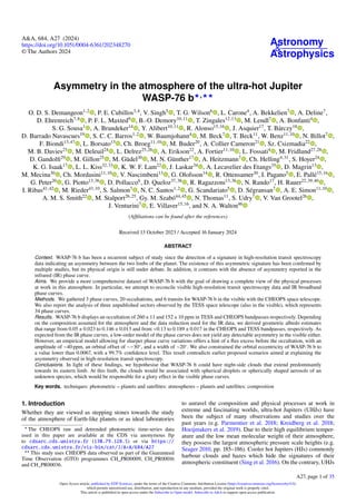
Asymmetry in the atmosphere of the ultra-hot Jupiter WASP-76 b

Astronomy
&
Astrophysics
A&A, 684, A27 (2024)
https://doi.org/10.1051/0004-6361/202348270
© The Authors 2024
Asymmetry in the atmosphere of the ultra-hot Jupiter
WASP-76 b⋆,⋆⋆
O. D. S. Demangeon1,2
, P. E. Cubillos3,4
, V. Singh5
, T. G. Wilson6
, L. Carone4
, A. Bekkelien7
, A. Deline7
,
D. Ehrenreich7,8
, P. F. L. Maxted9
, B.-O. Demory10,11
, T. Zingales12,13
, M. Lendl7
, A. Bonfanti4
,
S. G. Sousa1
, A. Brandeker14
, Y. Alibert10,11
, R. Alonso15,16
, J. Asquier17
, T. Bárczy18
,
D. Barrado Navascues19
, S. C. C. Barros1,2
, W. Baumjohann4
, M. Beck7
, T. Beck11
, W. Benz11,10
, N. Billot7
,
F. Biondi13,47
, L. Borsato13
, Ch. Broeg11,10
, M. Buder20
, A. Collier Cameron21
, Sz. Csizmadia22
,
M. B. Davies23
, M. Deleuil24
, L. Delrez25,26
, A. Erikson22
, A. Fortier11,10
, L. Fossati4
, M. Fridlund27,28
,
D. Gandolfi29
, M. Gillon25
, M. Güdel30
, M. N. Günther17
, A. Heitzmann7
, Ch. Helling4,31
, S. Hoyer24
,
K. G. Isaak17
, L. L. Kiss32,33
, K. W. F. Lam22
, J. Laskar34
, A. Lecavelier des Etangs35
, D. Magrin13
,
M. Mecina30
, Ch. Mordasini11,10
, V. Nascimbeni13
, G. Olofsson14
, R. Ottensamer30
, I. Pagano5
, E. Pallé15,16
,
G. Peter20
, G. Piotto13,36
, D. Pollacco6
, D. Queloz37,38
, R. Ragazzoni13,36
, N. Rando17
, H. Rauer22,39,40
,
I. Ribas41,42
, M. Rieder43,10
, S. Salmon7
, N. C. Santos1,2
, G. Scandariato5
, D. Ségransan7
, A. E. Simon11,10
,
A. M. S. Smith22
, M. Stalport26,25
, Gy. M. Szabó44,45
, N. Thomas11
, S. Udry7
, V. Van Grootel26
,
J. Venturini7
, E. Villaver15,16
, and N. A. Walton46
(Affiliations can be found after the references)
Received 13 October 2023 / Accepted 16 January 2024
ABSTRACT
Context. WASP-76 b has been a recurrent subject of study since the detection of a signature in high-resolution transit spectroscopy
data indicating an asymmetry between the two limbs of the planet. The existence of this asymmetric signature has been confirmed by
multiple studies, but its physical origin is still under debate. In addition, it contrasts with the absence of asymmetry reported in the
infrared (IR) phase curve.
Aims. We provide a more comprehensive dataset of WASP-76 b with the goal of drawing a complete view of the physical processes
at work in this atmosphere. In particular, we attempt to reconcile visible high-resolution transit spectroscopy data and IR broadband
phase curves.
Methods. We gathered 3 phase curves, 20 occultations, and 6 transits for WASP-76 b in the visible with the CHEOPS space telescope.
We also report the analysis of three unpublished sectors observed by the TESS space telescope (also in the visible), which represents
34 phase curves.
Results. WASP-76 b displays an occultation of 260±11 and 152±10 ppm in TESS and CHEOPS bandpasses respectively. Depending
on the composition assumed for the atmosphere and the data reduction used for the IR data, we derived geometric albedo estimates
that range from 0.05 ± 0.023 to 0.146 ± 0.013 and from <0.13 to 0.189 ± 0.017 in the CHEOPS and TESS bandpasses, respectively. As
expected from the IR phase curves, a low-order model of the phase curves does not yield any detectable asymmetry in the visible either.
However, an empirical model allowing for sharper phase curve variations offers a hint of a flux excess before the occultation, with an
amplitude of ∼40 ppm, an orbital offset of ∼−30◦
, and a width of ∼20◦
. We also constrained the orbital eccentricity of WASP-76 b to
a value lower than 0.0067, with a 99.7% confidence level. This result contradicts earlier proposed scenarios aimed at explaining the
asymmetry observed in high-resolution transit spectroscopy.
Conclusions. In light of these findings, we hypothesise that WASP-76 b could have night-side clouds that extend predominantly
towards its eastern limb. At this limb, the clouds would be associated with spherical droplets or spherically shaped aerosols of an
unknown species, which would be responsible for a glory effect in the visible phase curves.
Key words. techniques: photometric – planets and satellites: atmospheres – planets and satellites: composition
1. Introduction
Whether they are viewed as stepping stones towards the study
of the atmosphere of Earth-like planets or as ideal laboratories
⋆
The CHEOPS raw and detrended photometric time-series data
used in this paper are available at the CDS via anonymous ftp
to cdsarc.cds.unistra.fr (130.79.128.5) or via https://
cdsarc.cds.unistra.fr/viz-bin/cat/J/A+A/684/A27
⋆⋆
This study uses CHEOPS data observed as part of the Guaranteed
Time Observation (GTO) programmes CH_PR00009, CH_PR00016
and CH_PR00036.
to unravel the composition and physical processes at work in
extreme and fascinating worlds, ultra-hot Jupiters (UHJs) have
been the subject of many observations and studies over the
past years (e.g. Parmentier et al. 2018; Kreidberg et al. 2018;
Hoeijmakers et al. 2019). Due to their high equilibrium temper-
ature and the low mean molecular weight of their atmosphere,
they possess the largest atmospheric pressure scale heights (e.g.
Seager 2010, pp. 185–186). Cooler hot Jupiters (HJs) commonly
harbour clouds and hazes which hide the signatures of their
atmospheric constituent (Sing et al. 2016). On the contrary, UHJs
A27, page 1 of 35
Open Access article, published by EDP Sciences, under the terms of the Creative Commons Attribution License (https://creativecommons.org/licenses/by/4.0),
which permits unrestricted use, distribution, and reproduction in any medium, provided the original work is properly cited.
This article is published in open access under the Subscribe to Open model. Subscribe to A&A to support open access publication.

Demangeon, O. D. S., et al.: A&A, 684, A27 (2024)
tend to be cloud-free, at least on their day-sides (e.g. Parmentier
et al. 2018; Kitzmann et al. 2018). Thanks to the combination of
these two elements, UHJs are ideal targets for ground and space-
based observatories. Their atmospheres can be probed with most
of the available observational techniques, which provide a more
extensive view than any other class of exoplanets.
Dozens of atomic and molecular species, some ionised,
have already been detected in the atmosphere of UHJs (e.g.
Azevedo Silva et al. 2022; Borsa et al. 2021). We have also
seen a tremendous effort from the community to more closely
model the physical processes driving these atmospheres in an
attempt to explain the wealth of observational constraints (e.g.
the identification of hydrogen dissociation as a dominant heat
transport mechanism for UHJs; Bell & Cowan 2018; Tan &
Komacek 2019; Mansfield et al. 2020). One-dimensional (1D)
radiative transfer models embedded in Bayesian inference tools
have successfully modelled low-resolution and high-resolution
transmission spectroscopic observations. They have allowed us
to infer the presence of many species and retrieve abundance
ratios (e.g. Kitzmann et al. 2023; Pluriel et al. 2020; Gibson
et al. 2020; Brogi & Line 2019). Three-dimensional (3D) global
circulation models coupled with radiative transfer models and
other types of models capable of accounting for the spatial inho-
mogeneity of these atmospheres enabled the interpretation of
orbital phase curves (PCs) and minute line-shape deformations
(e.g. Kreidberg et al. 2018; Tan & Komacek 2019; Helling et al.
2021; Changeat et al. 2022; Jones et al. 2022; Seidel et al. 2023;
Pelletier et al. 2023).
WASP-76 b is (arguably) considered an archetypal UHJ
(West et al. 2016). From the ground, multiple studies have
reported the detection of close to 20 different species (primarily
atoms and ions), along with many more upper limits using
high-resolution spectroscopic observation in the visible and the
near infrared (NIR) obtained during transit (Tsiaras et al. 2018;
Seidel et al. 2019, 2021; Ehrenreich et al. 2020; Azevedo Silva
et al. 2022; Pelletier et al. 2023; Kesseli et al. 2020, 2022;
Sánchez-López et al. 2022; Gandhi et al. 2022; Kawauchi et al.
2022; Kesseli & Snellen 2021; Casasayas-Barris et al. 2021;
Landman et al. 2021; Deibert et al. 2021; Tabernero et al.
2021; Edwards et al. 2020). High-resolution observations in
the NIR taken close to occultation have shown the presence
of CO and hints of H2O emission lines indicative of the pres-
ence of a thermal inversion in the planet’s upper atmosphere
(Yan et al. 2023). Space-based observatories not only provided
low-resolution transit and emission spectroscopy, but also full
PC in the NIR and mid-IR (May et al. 2021; Fu et al. 2021;
Garhart et al. 2020; Tsiaras et al. 2018). This plethora of obser-
vations provides a unique opportunity to piece together one of
the most comprehensive views of an exoplanet’s atmosphere.
The scientific interest in UHJs and, in particular, WASP-76 b
has increased drastically after the detection and later confirma-
tion of the asymmetric signature coming from the two limbs of
WASP-76 b in transmission detected at ultra-high spectral reso-
lution (Ehrenreich et al. 2020; Kesseli & Snellen 2021; Pelletier
et al. 2023). Based on a toy model, Ehrenreich et al. (2020)
interpreted these observations as an asymmetry in the iron com-
position: the upper atmosphere of the morning limb (also called
leading limb or western limb) of WASP-76 b would be depleted
in gaseous iron compared to its evening limb (also called trail-
ing or eastern limb) due to the condensation of iron over the
night-side. Naturally, Savel et al. (2022), Wardenier et al. (2021)
and May et al. (2021) attempted to confront these observa-
tions with global circulation models (GCMs). All three studies
have agreed that standard GCM models cannot reproduce the
asymmetry detected by Ehrenreich et al. (2020). Savel et al.
(2022) and Wardenier et al. (2021) both argued that an asym-
metry in the composition of the limbs is not the only way to
explain the observations. Savel et al. (2022) invoked the presence
of clouds and a slight eccentricity of the planet’s orbit, while
Wardenier et al. (2021) highlighted the importance of tempera-
tures and wind dynamics. Both studies have argued that a weak
drag, or long drag timescale (from 105
to 107
s), would be neces-
sary to explain the asymmetry. May et al. (2021) took a slightly
different approach to the problem, as they also presented the IR
phase curves of WASP-76 b. The phase curves show little to no
asymmetry which indicates a strong drag, or short drag time-
scale (≤104
s), in contrast with the results of high-resolution
transmission spectroscopy.
In this paper, we provide new observational constraints on
the puzzling atmosphere of WASP-76 b with phase curve, tran-
sit, and eclipse observations in the visible with the CHEOPS and
TESS instruments (Sects. 2 and 4). We refine the properties of
WASP-76 a and its stellar companion WASP-76 b (Sect. 3). We
revisit the emission spectra of this planet (Sect. 5.1) and derive
its geometric albedo (Ag). We discuss the available phase curves
at visible and IR wavelengths (Sects. 5.2 and 5.2.2). Finally,
we argue that the visible phase curves of WASP-76 b hold cru-
cial elements to reach a comprehensive view of its atmosphere
(Sect. 6).
2. Datasets
2.1. CHEOPS
We observed WASP-76 b with CHEOPS during 29 separate vis-
its spread over 3 consecutive observability periods of WASP-76
as part of the CHEOPS Guaranteed Time Observations. We
first observed 2 full PC, 15 occultations, and 2 transits between
2020-09-09 and 2020-12-16. One year later, we observed
1 additional PC, 5 more occultations and 3 transits from
2021-09-05 to 2021-12-07. Finally, a year later, on 2022-09-18,
we observed 1 additional transit. The transits, occultations, and
PCs were observed as part of programs PR100009, PR100016,
and PR100036 respectively. The details of these observations are
provided in Appendix A and Table A.1.
The light curves were extracted using the CHEOPS data
reduction pipeline (DRP, Hoyer et al. 2020) version 13.1.0 which
relies on aperture photometry. As described in Benz et al. (2021),
CHEOPS data are affected by various instrumental trends.
These instrumental trends need to be addressed for an accu-
rate interpretation, especially when looking for astrophysical
signals of a few hundreds ppm, like planetary occultations and
PCs. CHEOPS is in a low-Earth Sun-synchronous orbit and also
spins around its line of sight. The orbital and roll motions are
synchronised, which allows the radiator to always point away
from Earth. Both motions introduce instrumental trends in the
CHEOPS data. The roll motion causes the field of view to
rotate around the line of sight. This introduces trends in the
photometry which typically correlate with the roll angle of the
spacecraft. Due to its orbital motion, CHEOPS orbits above
different regions of Earth with varying insolation and cloud
coverage. This will produce trends that correlate with the roll
angle but also with the background measured on the images. The
pixel response non-uniformity (PRNU) triggers another com-
mon source of instrumental trends. Due to pointing jitter, the
point spread function (PSF) of the target star slightly moves
on the charge coupled device (CCD) from exposure to expo-
sure and inaccuracies in the PRNU calibration produce trends
A27, page 2 of 35

in the photometry, which is correlated with the X and Y centroid
positions of the target PSF on the CCD. The last typical source
of instrumental trend is called the thermal ramp. CHEOPS is a
mono-target instrument and it changes pointing for each target.
This pointing change implies a change of solar illumination of
the telescope tube and mechanical structure, which produces a
temperature change and, in turn, the shape of the PSF changes.
These changes lead to photometric trends that are usually corre-
lated with the temperature measured by a sensor located on the
telescope tube (thermFront_2, e.g. Morris et al. 2021).
We mitigated these instrumental trends using cubic spline
decorrelations against the following decorrelation variables: the
roll angle of the spacecraft, X and Y centroid positions of the
target’s PSF on the CCD, background measured on the images,
and the temperature of the telescope tube. The spline decorrela-
tion is performed simultaneously with the fit of the astrophysical
model (see Sect. 4.1). It consists of fitting a cubic spline model
to the residuals of the astrophysical model versus the decorrela-
tion variable. In order to decorrelate against multiple variables,
we performed multiple spline fits sequentially. We started by
performing the spline decorrelation against the roll angle using
the same roll angle model for all visits. The residuals of this
fit were then used for another fit of X and Y centroid posi-
tions using a 2D spline model. Over the course of the three
seasons of observations, the location of the target stars on the
CHEOPS were purposefully changed to occupy the region of the
CCD that was the least affected by bad pixels at the time. Thus,
we used three different models for the different locations on
the CHEOPS CCD. This process was repeated two more times
to perform the spline decorrelation against the telescope tube’s
temperature and, finally, the measured background. In both of
these cases, each visit was modelled independently of the others.
The spline fits are implemented with the UnivariateSpline
and the SmoothBivariateSpline python classes of the
scipy.interpolate package for the 1D and 2D spline fits,
respectively (Virtanen et al. 2020). When performing the fit,
these two classes automatically selected the position of the knots.
The user can influence the number of knots with the smoothing
factor that we leave to None, which implies that this smoothing
factor is set according to the number of data points.
2.2. TESS
TESS (Ricker et al. 2015) observed WASP-76 during
sector 30 from 2020-09-22 to 2020-10-21 and one year later dur-
ing sectors 42 and 43 from 2021-08-20 to 2021-10-12 and we
retrieved the data through the MAST archive.
The data were extracted using the PDC-SAP photometry
and PSF-SCALPELS aperture photometry. In Appendix B.2, we
show a summary of our comparison of the two methods and jus-
tify our choice to use the PSF-SCALPELS photometry for the
rest of this paper. For the PSF-SCALPELS photometry, we com-
pute the shape change components of the TESS PSF following
the procedure outlined in Wilson et al. (2022) that has been suc-
cessfully shown to remove roll angle, contamination, and back-
ground effects in CHEOPS data (Hawthorn et al. 2023; Hoyer
et al. 2022; Parviainen et al. 2022). In brief, for each sector, we
conducted a principal component analysis (PCA) decomposition
of the auto-correlation of the calibrated target pixel file frames to
obtain a series of vectors that explain any variations in the PSF.
We selected the most significant components for inclusion in
the global analysis via a leave-one-out-cross-validation method.
For all sectors, we re-extracted the TESS photometry, using a
noise-optimised aperture photometry method (Wilson, in prep.).
These were background-corrected using custom sky-level masks,
scattered-light-corrected using a PCA on background pixels, and
jitter-corrected by detrending against co-trending basis vectors
(CBVs) and two-second cadence engineering quaternion mea-
surements following the approach in Delrez et al. (2021). We
then mitigate the potential residual trends by performing a spline
decorrelation simultaneously with the fit of the astrophysical
model. The procedure is similar to the one used for the spline
decorrelation of the CHEOPS data (see Sect. 2.1). For TESS,
instead of using a roll angle, X and Y centroid position, temper-
ature, and background, we have used the vectors resulting from
the PCA decomposition of the auto-correlation of the calibrated
images.
2.3. HST
HST observed WASP-76 b during four transits and one occul-
tation. The first transit visit was obtained on 2015-11-26 using
the WFC3 instrument with the G141 grism as part of program
ID 14260 (PI: Deming). The remaining three transit visits were
observed with the STIS instrument as part of program ID 14767
(PI: López-Morales & Sing): 2016-11-16 and 2017-01-17 with
the G430L grism and 2017-02-19 with the G750L grism. The
only occultation visit was obtained with the G141 grism of the
WFC3 instrument on 2016-11-03 as part of program ID 14767.
These data were already analysed and published in three papers.
von Essen et al. (2020) analysed the STIS transit data only.
Edwards et al. (2020, hereafter E20) analysed the WFC3 data
only. Finally, Fu et al. (2021, hereafter F21) combined all HST
(STIS and WFC3) data and the Spitzer transits and occultations
(see Sect. 2.4).
We decided not to re-reduce the data and to rely on the
published analyses of this dataset. Our focus was set in the occul-
tation visits in order to model the thermal SED of WASP-76 b’s
day-side (see Sects. 5.1.2 and 6.1). Therefore, we mostly set aside
the STIS data and concentrated on the WFC3 data. The two
reductions provided by F21 and E20 are not compatible and, as
such, we compared the impact of the two data reductions on our
analysis (see Sects. 5.1.2 and 6.1). We provide more details on
the different reductions of the HST data in Appendix B.3.
2.4. Spitzer
Spitzer observed WASP-76 b during two occultations and three
phase curves with the InfraRed Array Camera (IRAC, Fazio
et al. 2004). The two occultations were acquired as part of the
program 12085 (PI: Drake Deming). One was observed in the
3.6 µm channel (CH1 or IRAC1) on 2016-03-22, and the other
in the 4.5 µm channel (CH2 or IRAC2) on 2016-04-01. The three
phase curves were acquired as part of program 13038 (PI: Kevin
Stevenson). The first one was observed in the 4.5 µm channel on
2017-04-17 and the two others were observed in the 3.6 µm chan-
nel on 2017-05-03 and 2018-04-23. These data have already been
published by Garhart et al. (2020), F21 and May et al. (2021).
However, due to the particularities of the data reduction of the
Spitzer data, we chose to re-reduce and re-analyse them. These
data were downloaded from the Spitzer Heritage Archive1
.
The reduction and analysis processes applied to these
datasets are similar to the approach in Demory et al. (2016b),
where we modelled the IRAC intra-pixel sensitivity (Ingalls
et al. 2016) using a modified implementation of the BLISS
(BiLinearly-Interpolated Sub-pixel Sensitivity) mapping algo-
rithm (Stevenson et al. 2012). In addition to the BLISS mapping
1 http://sha.ipac.caltech.edu
A27, page 3 of 35

Table 1. Main parameters inferred from the Spitzer, TESS, and CHEOPS light curves
Model Bandpass Rp/R∗
(a)
A0
(a,b)
ϕ0
(b) ∆F
F eclipse
(a)
Fnight
(a)
(%) (ppm) (◦
) (ppm) (ppm)
Cos IRAC2 10.985 ± 3.4 × 10−2
2174 ± 46 −0.5 ± 1.0 3633+40
−42 1459 ± 47
Kelp,therm IRAC2 10.989 ± 3.4 × 10−2
2203+46
−50 −3.4 ± 1.0 3646+43
−41 1453+44
−51
Garhart+20 IRAC2 – – – 3762 ± 92 –
Fu+21 IRAC2 11.351 ± 5.6 × 10−2
– – 3665 ± 89 –
May+21 IRAC2 10.6 2928 ± 76 −0.67 ± 0.2(c)
3729 ± 52 –
Cos IRAC1 10.735 ± 2.7 × 10−2
– – 2722+72
−65 –
Kelp,therm IRAC1 10.684 ± 2.7 × 10−2
– – 2632 ± 71 –
Garhart+20 IRAC1 – – – 2979 ± 72 –
Fu+21 IRAC1 10.862 ± 4.1 × 10−2
– – 2988 ± 65(d)
–
May+21 IRAC1 10.048 804.0 ± 42.5 −0.68 ± 0.48(c)
2539 ± 30 –
Cos TESS 10.883 ± 1.3 × 10−2
251 ± 11 −4.6 ± 2.2 260 ± 11 <37
Cos+Gauss TESS 10.884 ± 1.3 × 10−2
223+17
−21 −0.6+3.5
−3.8 231 ± 18 <37
Cos+Kelp,refl TESS 10.885 ± 1.3 × 10−2
224+18
−19 −2.6+2.8
−3.5 233 ± 18 <36
Cos CHEOPS 10.923 ± 9.4 × 10−3
143 ± 11 −7.6+5.1
−5.4 152 ± 10 <38
Gauss+Gauss(e)
CHEOPS 10.927 ± 9.0 × 10−3
141 ± 18 −2.3+7.5
−5.9 122 ± 26 <46
Cos+Kelp,refl CHEOPS 10.919 ± 10.0 × 10−3
120+19
−21 −2.6+6.2
−8.2 122 ± 26 <42
Notes. As mentioned in Sect. 4.2, when an estimate and uncertainty are provided, it corresponds to the median and the 68% confidence interval
estimated with the 16th and 84th percentiles of the posterior probability density function. When an upper limit is provided, it corresponds to the
99.7th percentile. (a)
All relative fluxes are provided corrected from the contamination factor of the light curve. (b)
For the Cos+Gauss and the
Gauss+Gauss phase curve models, this table only reports the characteristics of the first and main component of the models: the cosine for the
Cos+Gauss model and the first Gaussian function, the one with the largest width, for the Gauss+Gauss model. The characteristics of the second
component, Gaussian in both models, are reported in Table 4. (c)
We caution the reader that the values provided in this table for May+21 are
the opposite of the ones provided in their paper due to the difference in convention used for the phase curve offset (see Sect. 4.1). (d)
F21 found
variations in the occultation depth measured from the three occultations observed in the IRAC1 channel. The value provided here is the average
of these three measurements. We do not find such variability in our data analysis. (e)
The Gauss+Gauss phase curve model used for the CHEOPS
phase-curve has an additional parameter: the standard deviation (σ0, see Eq. (3)) which quantifies the width of the primary and broadest Gaussian
which is estimated at 49 ± 7◦
.
(BM), our initial baseline model included a quadratic function
of the PRF’s full width at half maximum (FWHM) along the
x and y axes, which significantly reduces the level of corre-
lated noise as shown in previous studies (e.g. Lanotte et al. 2014;
Demory et al. 2016a,b; Gillon et al. 2017; Mendonça et al. 2018;
Barros et al. 2022; Jones et al. 2022). We further found that
including the background in the baseline model improved the
fit slightly (∆BIC=3). This baseline model (BM + PRF FWHM2
+ BKG) does not include time-dependent parameters. We imple-
mented this instrumental model in a Markov chain Monte Carlo
(MCMC) framework already presented in the literature (Gillon
et al. 2012). We included all data described in the paragraph
above in the same fit. We ran two chains of 200 000 steps each
to determine the corrected light curves at 3.6 and 4.5 µm that we
later used in our study.
As already pointed out by May et al. (2021), we found that
the 3.6 µm phase-curve parameters were very sensible to the
choice of the instrument baseline model. We identified differ-
ences in excess of 2 σ, in particular when increasing the order of
the polynomial function of the FWHM along the Y axis from 1
to 3, which exhibits large variations in both of the 3.6 µm vis-
its. The observed FWHM variations have timescales similar to
the planetary phase-curve signal, which complicates a robust
identification of the latter from instrumental correlated noise.
Equally concerning is the impact of data trimming at the begin-
ning of the longer astronomical observation requests (AORs) on
the phase-curve parameters, where differences between 0-min
and 30-min trimming are beyond 1 σ (see also May et al. 2021).
For these reasons, we elect to retain only the 3.6 µm transit and
occultations for the subsequent analysis.
A closer examination of the 4.5 µm data revealed that while
the inclusion of the background in our baseline model only
slightly improved the BIC (∆BIC=3), it significantly impacted
the phase curve amplitude which varied by more than 1 σ. We
found that the background as well as the PRF FWHM along the
x-axis are both correlated with the flux, on timescales that are
degenerate with the planetary phase-curve modulation signal.
Using a quadratic function of the PRF FWHM and/or includ-
ing the background in the instrumental model thus impacts the
phase curve parameters. Finally, we implemented a baseline
model using the noise pixel parameter (Mighell 2005; Lewis
et al. 2013), which yielded phase-curve amplitude and offset in
agreement with our adopted model described above (BM + PRF
FWHM2
+ BKG). This result speaks to the reliability of our
approach for this channel. However, it doesn’t remove the degen-
eracies and probably explains the diversity of the results obtained
from the analysis of this dataset (see Sects. 4.3, 5.1.2, and 5.2.1,
and Tables 1–3).
A27, page 4 of 35

Table 2. Day-side and night-side temperatures.
Model Bandpass Tnight Tday
(K) (K)
Cos IRAC2 1716 ± 27 2761 ± 30
Kelp,therm IRAC2 1670+20
−23 2623 ± 20
Garhart+20 IRAC2 – 2747 ± 60
May+21 IRAC2 1259 ± 44 2699 ± 32
Cos IRAC1 –(a)
2579 ± 37
Kelp,therm IRAC1 –(a)
2489 ± 35
Garhart+20 IRAC1 – 2669 ± 57
May+21 IRAC1 1518 ± 61 2471 ± 27
Cos TESS –(b)
2723 ± 22
Cos CHEOPS –(b)
3002 ± 27
Notes. (a)
We did not derive night-side temperature in the Spitzer IRAC1
bandpass due to the unreliability of the phase curve extraction (see
Sect. 2.4). (b)
We did not derive night-side temperatures in the TESS
and CHEOPS bandpasses because the night-side flux was not detected
in these bandpasses (see Fnight measurements in Table 1).
3. Stars: WASP-76 a and b
We determined the radius of WASP-76 a by using a mod-
ified MCMC IR flux method (MCMC IRFM; Blackwell &
Shallis 1977; Schanche et al. 2020) that computes the appar-
ent bolometric flux via a comparison of observed and synthetic
broadband photometry that is converted to the stellar effective
temperature and angular diameter. This yields the radius when
combined with the parallax. For the WASP-76 system, we com-
puted the synthetic broadband photometry by building a spectral
energy distribution (SED) with the ATLAS Catalogues (Castelli
& Kurucz 2003) of atmospheric models and two stellar compo-
nents; the primary using the spectral parameters derived from
ESPRESSO spectra by Ehrenreich et al. (2020) and the compan-
ion with parameters taken from the literature (Ngo et al. 2016;
Bohn et al. 2020; Southworth et al. 2020; May et al. 2021) and
empirical relations (Baraffe et al. 2015). By fitting the combined
models to observed data taken from the most recent data releases
for the following bandpasses; Gaia G, GBP, and GRP, 2MASS J,
H, and K, and WISE W1 and W2 (Skrutskie et al. 2006; Wright
et al. 2010; Gaia Collaboration 2023), and using the offset cor-
rected Gaia DR3 parallax (Lindegren et al. 2021), we obtained
a stellar radius of R⋆ = 1.764 ± 0.036 R⊙. By fitting both stel-
lar components of the SED to observed data, this approach also
allows us to compute the contamination factor of the companion
in our photometric light curve data, which is the percentage of
the light collected in the photometric aperture that corresponds
to the companion. Assuming that the light of both WASP-76 a
and b are entirely captured by the photometric aperture, we found
contamination factors in the TESS, CHEOPS, and IRAC 1 and
2 bandpasses of 0.037±0.002, 0.028±0.001, 0.095±0.005, and
0.090±0.004, respectively. We also derived the contamination
factor coefficients for the HST-WFC3 bandpasses used by E20
that are provided in Table B.1.
Taking Teff, [Fe/H], and R⋆ (along with their uncertainties)
as the input parameters, we finally determined the isochronal
mass M⋆ and age t⋆ by using two different stellar evolution-
ary models. In detail, we retrieved a first pair of mass and age
estimates thanks to the isochrone placement algorithm (Bonfanti
et al. 2015, 2016), which interpolates the input parameters within
pre-computed grids of PARSEC2
v1.2S (Marigo et al. 2017)
tracks and isochrones. A second pair of estimates, instead, is
computed ‘on-the-fly’ by the CLES (Code Liègeois d’Évolution
Stellaire; Scuflaire et al. 2008) code, which generates the best-fit
evolutionary track accounting for the input constraints through
the Levenberg-Marquardt minimisation scheme (Salmon et al.
2021). Once the two pairs of mass and age estimates were avail-
able, we checked their mutual consistency via the χ2
-based
criterion as detailed in Bonfanti et al. (2021) and we finally
merged the results, which yielded the following robust estimates:
M⋆ = 1.427+0.075
−0.080 M⊙ and t⋆ = 2.4+0.3
−0.5 Gyr.
4. Light-curve fitting
4.1. Transit, occultation, and phase-curve and instrumental
models
Our dataset includes planetary transits, PCs, and occultations.
For the transits and occultation models, we use the model pro-
vided by the batman Python package (Kreidberg 2015). The
transit model takes as its input the planetary orbital parameters,
the planet over star radius ratio (Rp/R∗) and the four coeffi-
cients of the non-linear limb-darkening model (u1, u2, u3, u4).
Additionally, the occultation model implemented in batman also
requires the planet over star flux ratio (Fp/F∗) that drives the
amplitude of the occultation. However, when the occultation is
observed as part of, or in combination with a PC, we fix the
flux ratio and the out-of-occultation flux to 1 and the occultation
model is multiplied by the PC model. The occultation depth is
thus defined by the PC’s amplitude at superior conjunction. The
parametrisation that we used for the orbital parameters includes
the stellar density (ρ∗), the planetary orbital period (P), the time
of inferior conjunction (tic), the products of the planetary orbital
eccentricity by the cosine and sine of the argument of periastron
passage of the planet’s orbit (e cos ω, e sin ω), and the cosine of
the planetary orbital inclination (cos i).
We used five different models for the PC. The first model,
FCos, is an empirical model which models the phase curve
variations with a cosine function and is described by
FCos = Fn +
A0
2
· cos
"
2π
P
(t − tic) − ϕ0 + π
#
. (1)
The first term, Fn, quantifies the ratio of the planetary night-
side flux over the stellar flux while the second term describes
the phase variations with a cosine function of amplitude A0 and
phase offset ϕ0.
The second model, FCos+Gauss, is another empirical model
which adds a Gaussian to the cosine phase curve model to cap-
ture sharp features that the cosine function cannot (see Sect. 4.3).
The expression for this model is
FCos+Gauss = FCos + A1 · exp






(ϕ − ϕ1)2
2 ∗ σ2
1





 , (2)
where A1 is the amplitude of the Gaussian component, ϕ1 is the
planetary orbital phase around which this component is cen-
tred and σ1 is the standard deviation, quantifying the width
of the Gaussian component. The orbital phase ϕ is defined as
2π[(t − tic)%P − 0.5], where % is the modulo operator meaning
that ϕ is ± π at mid-transit and equal to zero at half a period after
mid-transit (at mid-eclipse for circular orbits).
2 PAdova and TRieste Stellar Evolutionary Code: http://stev.
oapd.inaf.it/cgi-bin/cmd
A27, page 5 of 35

Table 3. WASP-76 b’s Ag estimates.
Datasets
Bandpass Species(a)
D1: HST (E20) D2: HST (E20) + Spitzer (this work) D3: HST + Spitzer (F21)
CHEOPS
with TiO/VO 0.073 ± 0.023 0.117 ± 0.013 0.145 ± 0.014
without TiO 0.111 ± 0.015 0.117 ± 0.014 0.146 ± 0.013
without TiO/VO 0.112 ± 0.014 0.116 ± 0.013 0.146 ± 0.013
TESS
with TiO/VO <0.13 0.114 ± 0.018 0.188 ± 0.017
without VO 0.104 ± 0.022 0.115 ± 0.018 0.189 ± 0.017
without TiO/VO 0.106 ± 0.020 0.114 ± 0.017 0.189 ± 0.017
Notes. When an upper limit of Ag is provided, it corresponds to the upper limit of the 99.7% confidence interval. Otherwise, the value provided
is the median of the posterior distribution and the uncertainties correspond to the 16 and 84th percentiles. (a)
The full list of species involved in the
retrieval, besides TiO and VO, is described in Sect. 5.1.
We also used a third model, FGauss+Gauss, in an attempt to
better capture the shape of the CHEOPS phase curve: a shape
which seems to be composed of a broad feature which is a bit
sharper than a cosine function and a second even sharper feature.
More details are provided in Appendix B.1. The expression for
this model is
FGauss+Gauss = Fn + A0 · exp






(ϕ − ϕ0)2
2 ∗ σ2
0





 + A1 · exp






(ϕ − ϕ1)2
2 ∗ σ2
1





 .
(3)
The fourth and fifth models are physically driven and aim at
confronting physical hypothesis against the observed data. The
fourth model, Kelp,therm, is designed to represent the thermal
PC and uses the implementation provided by the kelp Python
package (Morris et al. 2022). It describes the two-dimensional
thermal brightness map of the exoplanet using parabolic cylin-
der basis functions which are a generalisation of the spherical
harmonics. This set of functions has been shown by Heng
& Workman (2014) to be adequate solutions to the equations
describing the thermal behaviour of hot gas giants. Morris
et al. (2022) have also shown that they can reproduce the out-
puts of general circulation models with enough precision for
most current applications. Following the recommendations of
Morris et al. (2022), we use only the basis function (Cl,m) of
degree l = 1 and order m = 1. We also fixed the dimensionless
fluid number (α) to 0.6, the dimensionless drag frequency (ωdrag)
to 4.5 and the input bond albedo (A′
B) to 0. We refer the reader to
Morris et al. (2022) and reference therein, Heng & Workman
(2014) in particular, for a more detailed explanation of these
quantities. Besides the occultation model’s parameter and the
fixed parameters that we just mentioned, this model depends on
a few additional parameters: the greenhouse factor (f′
), the plan-
etary orbital phase offset (ϕKelp) and the amplitude of the basis
function of degree and order 1 (C1,1). We note that ϕKelp is not
exactly equivalent to the traditional hotspot offset as represented
by ϕ0 in the cosine model. However, for values of ωdrag ≳ 3,
we fixed it to 4.5 and found that the difference between the two
is negligible (Morris et al. 2022). Finally, Kelp,therm requires
us to specify the stellar spectrum and spectral transmission of
the observations. For the stellar spectrum, we use a synthetic
spectrum generated with the PHOENIX-ACES-AGSS-COND code
by Husser et al. (2013) with an effective temperature (Teff) of
6300 K and a log g of 4.5 (see Sect. 3).
The fifth model, Kelp,refl, is designed to represent the
reflected light PC produced by a planet with inhomogeneous
reflective properties. It uses the implementation provided by the
same kelp Python package, but described in Heng et al. (2021).
The planetary day-side is decomposed into two regions that
reflect light according to the Henyey-Greenstein law. One region
has a low or baseline reflectivity characterised by a single scat-
tering albedo ω0 and spans between the two longitudes x1 and
x2. The other region, which occupies the rest of the day-side, has
an increased reflectivity described by a single scattering albedo
equals to ω0 + ω′
where ω′
is a positive number. This model also
use Ag as parameter. From Ag, ω0, ω′
, x1, x2, we can compute
the scattering asymmetry (g) which is assumed to be identical in
both regions. A value of g of –1, 0 and 1 corresponds to purely
reverse, isotropic and forward scattering respectively (Heng et al.
2021).
Regarding the impact of the instruments on the data, we
divided the model into two components, one that is specific to
each instrument and which was described in the sections spe-
cific to each instrument (Sects. 2.1, 2.2, 2.4) and the other which
is identical for each instrument. For all instruments, we need to
account for the contamination of the light curve, also called 3rd
light, coming from other stars than the target. This contamina-
tion can be considered as an instrumental effect as it can heavily
depend on the angular resolution of the instrument. As such, we
introduce a contamination factor parameter (c) for each instru-
ment. The astrophysical models of the light curve described in
the previous paragraphs are multiplied by (1 − c) to account for
the effect of contamination. In our case and for all instruments,
the contamination of the light curve is completely dominated
by the contamination due to WASP-76 b that we estimated in
Sect. 3. Another aspect common to all instruments is the pho-
tometric offset. All the astrophysical models mentioned before
assume that the light curve is normalised. In the absence of stel-
lar activity, this means that the stellar flux is equal to 1 in relative
flux. The normalisation of the light curves performed prior to
their modelling is rarely accurate enough. To mitigate that, for
each instrument, we introduce a photometric offset parameter
((∆F/F)∗) that is added to the light curve model (including the
contamination and the rest of the astrophysical model) to account
for an imperfect normalisation.
4.2. Fitting procedure
In order to fit the models to the data, we maximised the poste-
rior probability of the model parameters. The likelihood involved
in the posterior computation is a Gaussian likelihood with a jit-
ter parameter (σinst) that is added in quadrature to the data’s error
bars (Baluev 2009). We used one jitter parameter per instrument.
The priors on the parameters were chosen to reflect physical
A27, page 6 of 35

Fig. 1. Reduced and phase-folded light-curves in CHEOPS, TESS, Spitzer-IRAC1 and Spitzer-IRAC2 bandpasses: The light-curves are corrected
from the contamination and from modelled instrumental systematic. The zero flux level is set as the stellar flux, except for the Spitzer-IRAC1 data
where, in the absence of a reliable PC, we set the out-of-transit and the out-of-eclipse flux level to zero. Here, we only show the data acquired
around occultations. The grey points are the individual measurements. The red ones are their mean values within orbital phase bins regularly
distributed. The solid red line represents the best model (see Sect. 4.2) using the cosine phase-curve model (described in Sect. 4.1). The solid blue
and orange lines represent the two GCM models with low and high friction (see Sect. 5.2.2). Top: light curves displayed focusing on the transit.
Bottom: focus on the PCs.
boundaries or prior knowledge of the system from datasets inde-
pendent of the ones used in this paper. The priors are described
in more detail in Appendix D. In order to efficiently explore
the parameter space and find and explore the vicinity of the
global maximum of the posterior, we used the Python software
emcee, which implements the affine invariant Markov chain
Monte Carlo (MCMC) Ensemble sampler (Goodman & Weare
2010; Foreman-Mackey et al. 2013). We checked the conver-
gence of the exploration using a modified version of the Geweke
convergence criterion adapted to the multiple MCMC chains
that emcee provides (Geweke 1992). We only conserved the
iterations obtained after convergence. The best value of each
parameter is defined as the 50th percentile of the converged itera-
tions. As a consequence, we defined our best model as the model
for which the value of each parameter is set to the best value.
For the 68 % confidence interval, we use the 16th and 84th
percentiles.
4.3. Results
We first fit separately all the data obtained by each instrument
using the cosine model for the PC. The instrumental models
are described in Sect. 2 and the astrophysical models in
Sect. 4.1. Figure 1 presents the reduced and phase-folded data
of CHEOPS, TESS, Spitzer-IRAC1, and IRAC2 channels with
the best models. Table 1 summarises the main results. The full
table with all inferred parameters is provided in Appendix D.
We then fit the Spitzer-IRAC1 and Spitzer IRAC2 data with
the Kelp,therm PC model (see Sect. 4.1) to provide a more physi-
cally motivated fit of the Spitzer PCs which will help the physical
interpretation of the phase curves in terms of day and night-
side temperature, Bond albedo, and redistribution factor that will
be discussed in Sect. 5.2.1. Table 1 provides the main quan-
tities obtained from the fit and the full table with all inferred
parameters is provided in Appendix D.
The TESS and CHEOPS phase curves both display a flux
excess before the eclipse (see Fig. 1). The width of this
flux excess appears too small to be properly captured by the
Cos or Kelp therm models. As such, we perform an addi-
tional fit of these data using the Cos+Gauss model for TESS
and Gauss+Gauss model for CHEOPS, see Appendix B.1 for
more details on the choice of models. Figure 2 presents the
phase-folded light curves resulting from these fits. Table 1
A27, page 7 of 35

Fig. 2. Reduced and phase-folded light-curves in CHEOPS and TESS bandpasses using the Cos+Gauss and Gauss+Gauss phase curve models:
light-curves are corrected from the contamination and from modelled instrumental systematic. The zero flux level is set as the stellar flux. The
grey points are the individual measurements. The red ones are their mean values within orbital phase bins regularly distributed. The solid black
line represents the best model (see Sect. 4.2) using the Gauss+Gauss phase-curve model for CHEOPS and the Cos+Gauss model for TESS (both
described in Sect. 4.1). The top two panels present the reduced phase-folded light curve of and residuals of the CHEOPS data and the bottom two
panels are for the reduced phase-folded light curve of and residuals of the TESS data.
presents the main quantities obtained from this fit that corre-
spond to the first and widest component of both models. The
quantities specific to the second narrowest component of the
model are presented in Table 4. These results are discussed in
Sect. 6.2 and the full table of inferred parameters is provided in
Appendix D.
We also attempt to fit a more physically motivated model to
the TESS and CHEOPS phase curves using a combination of the
cosine model for the thermal contribution and a Kelp,refl model
for the reflected light component. Figure 3 presents the phase-
folded light curves resulting from these fits. Table 1 presents
the main quantities obtained from this fit that correspond to the
cosine components and the quantities specific to the Kelp,refl
component of the model are presented in Table 5. These results
are discussed in Sect. 6.2 and the full table of inferred parameters
is provided in Appendix D.
A27, page 8 of 35

Table 4. Parameters of the second component of the Cos+Gauss and
Gauss+Gauss PC models inferred from the TESS and CHEOPS light
curves.
Model Bandpass A1 ϕ1 σ1
(ppm) (◦
) (◦
)
Cos+Gauss TESS 39 ± 23 −34+18
−13 27 ± 14
Gauss+Gauss CHEOPS 47 ± 28 −31+11
−5 14+10
−8
Notes. This table only reports the characteristics of the second
component, the one with the smallest width, of the Cos+Gauss and
Gauss+Gauss models. This second component is a Gaussian in both
models. The characteristics of the first component are reported in
Table 1.
Finally, in order to derive the most precise constraints on the
orbits of WASP-76 b, we perform a fit of all the datasets together
(CHEOPS, TESS, IRAC1 and IRAC2). We adopt the Cos phase
curve model as it is the one with the lowest number of parameters
and which is the least costly computationally. The full table of
retrieved parameters is provided in Appendix D.
5. 1D and 3D atmospheric models
5.1. 1D emission spectra modelling
5.1.1. Modelling framework
We characterised the atmospheric properties of WASP-76 b by
applying a suite of atmospheric retrievals constrained by the
observed occultation spectra of the planet. To this end, we
employed the open-source PYRAT BAY modelling framework
(Cubillos & Blecic 2021), which enables atmospheric mod-
elling, spectral synthesis, and atmospheric Bayesian retrievals.
The atmospheric model consists of 1D parametric profiles of
the temperature, volume mixing ratios (VMR), and altitude as
a function of pressure. Our atmospheric model for WASP-76 b
extends from 10−9
to 100 bar. For the temperature profile model,
we adopted the prescription of Guillot et al. (1996). We modelled
the composition under thermochemical equilibrium according to
the temperature, pressure, and elemental composition at each
layer. We adopted a network of 45 neutral and ionic species
that are the main bearers of H, He, C, N, O, Na, Si, S, K, Ti,
V, and Fe. We parameterised the chemical model by the ele-
mental abundance of carbon, oxygen, and all other metals with
respect to solar values (labelled [C/H], [O/H], [M/H], respec-
tively). Finally, we computed the altitude of each layer assuming
hydrostatic equilibrium.
For each atmospheric model, PYRAT BAY then computes
the emission spectrum considering opacities from alkali lines
(Burrows et al. 2000), Rayleigh scattering (Kurucz 1970),
collision-induced absorption (Borysow et al. 1988, 1989, 2001;
Borysow & Frommhold 1989; Borysow 2002; Jørgensen et al.
2000), H−
bound-free and free-free opacity (John 1988), exo-
mol molecular line lists for H2O, NH3, HCN, TiO, and VO
(Tennyson et al. 2016), and HITEMP molecular line lists for
CO, CO2, and CH4 (Rothman et al. 2010). To process the large
molecular line-list opacity files, we applied the REPACK package
(Cubillos 2017) to extract the dominant line transitions. To man-
age the atmospheric retrieval exploration PYRAT BAY uses the
MC3 package (Cubillos et al. 2017), in this case using the Nested-
sampling algorithm implemented via PyMultiNest (Feroz et al.
2009; Buchner et al. 2014).
The main goal of these retrieval analyses is to disentan-
gle the thermal emission from the reflected light component of
the occultation depths, with which we can later infer the Ag of
WASP-76 b (see Sect. 6.1). Since our retrieval framework does
not account for reflected light, we conducted the retrieval anal-
yses only using the IR (longer wavelength) HST WFC3 and
Spitzer occultation measurements, where the emission spectrum
is dominated by thermal emission. Then as a post-process step,
we derived from the retrieval posterior distributions the model-
expected thermal emission at the CHEOPS and TESS bands. The
residuals between the observed and thermal-modeled depths are
then the planetary reflected light, which constrains the Ag (see
Sect. 6.1).
Given the significant differences between the occulta-
tion depths derived from the HST and Spitzer observations
(Appendix B.3 and Sect. 2.4), we opted to run retrieval analy-
ses for three data sets: Dataset 1 (D1) includes only the HST
WFC3 depths from E20. Dataset 2 (D2) includes the HST WFC3
depths from E20 and our Spitzer depths. Lastly, dataset 3 (D3)
includes the HST WFC3 and Spitzer depths from Fu et al. (2021).
This enabled us to perform a comprehensive exploration of the
plausible physical scenarios for WASP-76 b, as well as compare
our results to those of the literature.
Finally, we considered different scenarios for the presence
of TiO and VO in the atmosphere. These molecules are strong
absorbers in the optical and can significantly alter the emission
spectrum (Fortney et al. 2008); however, an unambiguous detec-
tion of these species has remained largely elusive, even for some
of the most highly irradiated planets (Hoeijmakers et al. 2022).
It is possible that these heavy molecules condense out of the
observable atmosphere in what is called a cold trap (Lodders
2002; Spiegel et al. 2009). Therefore, we ran retrieval analyses
considering three scenarios: with TiO and VO, with VO only
(motivated by Pelletier et al. 2023), and without TiO and VO.
5.1.2. Retrieval results
Figure 4 shows the retrieved spectra and temperature profiles
for the retrievals including TiO and VO opacity. Each one of
the three datasets leads to different spectra and thermal struc-
tures. To interpret these results we need to understand how the
absorbers impact the thermal emission spectrum. The WFC3
wavelength range is dominated by a strong H2O opacity band at
λ > 1.32 µm. A thermal inversion would then lead to a higher
brightness temperature at these longer wavelengths since the
stronger H2O opacity makes the atmosphere opaque at higher
altitudes (i.e. the H2O features show as emission bands). In
contrast, without a thermal inversion, the H2O bands show as
absorption bands, and the emission at longer wavelengths will
have a brightness temperature lower than that at the shorter
wavelengths.
The retrieval of the D1 dataset, which considers only the
HST/WFC3 occultation depths from E20, produce a thermal
inversion since the depths over the H2O band have brightness
temperatures slightly larger than those at the shorter wavelengths
(see Fig. 5). Consequently, the contribution functions show that
the WFC3 bands probe the pressures where the temperature
inversion occurs (∼10−2
bar).
When adding the Spitzer occultations from this work to the
retrieval constraints (D2 dataset), we obtained a non-inverted
thermal profile. This occurs because the Spitzer depths (in par-
ticular at 3.6 µm) have noticeably lower brightness temperatures
than the WFC3 depths, requiring absorption bands from carbon-
based species (mainly CO and CH4). This is shown by the Spitzer
A27, page 9 of 35

Fig. 3. Reduced and phase-folded light-curves in CHEOPS and TESS bandpasses using the Cos+Kelp,Refl phase curve models. As in Fig. 2, the
light-curves are corrected from the contamination and from modelled instrumental systematic. The zero flux level is set as the stellar flux. The
grey points are the individual measurements. The red ones are their mean values within orbital phase bins regularly distributed. The solid black
line represents the best model (see Sect. 4.2) using the Cos+Kelp,refl phase-curve model for CHEOPS and TESS (described in Sect. 4.1). The
top two panels present the reduced phase-folded light curve of and residuals of the CHEOPS data and the bottom two panels are for the reduced
phase-folded light curve of and residuals of the TESS data.
depths sitting below the blackbody model at T = 2630 K (dashed
grey curve) consistent with the E20 depths. In this case, the
WFC3 depths probe pressures where the atmosphere is nearly
isothermal. Considering the noticeable scatter in the E20 depths
and their relatively weak statistical evidence for a thermal inver-
sion (not a strong variation in brightness temperatures) it is not
unexpected for the retrieval to prefer the non-inverted solution.
This suggests that the Spitzer and HST data are incompatible to
some degree.
Finally, when retrieving the F21 dataset (D3), we find the
opposite scenario as for D2. Now the Spitzer depths have larger
brightness temperatures than the WFC3 depths, leading the
retrieval toward thermal inversion profile, while also remaining
largely isothermal over the pressures probed by WFC3. Although
A27, page 10 of 35

Table 5. Parameters of the Kelp,refl component of the Cos+Kelp,refl model inferred from the TESS and CHEOPS light curves.
Model Bandpass Ag g ω0 x1
(a)
x2
(a)
ω′
ω0 + ω′
(◦
) (◦
)
Cos+Kelp,refl TESS
<0.16 −0.37+0.22
−0.40 <0.15 <−75 40+29
−34 <0.6 >0.5
0.119+0.17
−0.048 0.083+0.172
−0.064 −79.7+8.3
−7.2 0.47+0.29
−0.31 0.62+0.26
−0.33
Cos+Kelp,refl CHEOPS
0.101+0.047
−0.036 −0.50+0.16
−0.20 <0.07 <−77 42+29
−48 0.30+0.24
−0.17 0.36+0.24
−0.17
0.047+0.045
−0.032 −81.1+8.4
−6.7
Notes. This table only reports the characteristics of the Kelp,refl component. The characteristics of the cosine component are reported in Table 1.
Several marginalised posteriors are not Gaussian and mostly provide upper/lower limits. In these cases, we provide in this table the 68th percentile
as upper limit or the 32nd percentile as lower limit, but we also provide the median and the border of the 68% confidence interval, as described in
Sect. 4.2, as the combination of the two allows us to better describe the posterior. (a)
x1 and x2 are defined such that −90◦
and 90◦
correspond to the
western and eastern terminators respectively.
Fig. 4. WASP-76 b occultation atmospheric retrievals. Left: light blue, dark blue, and orange curves and their associated shaded areas show the
retrieved spectrum and 68% credible intervals when fitting the D1, D2, and D3 occultation observations, respectively (see legends). These retrievals
include both TiO and VO opacities. The blue, red, and purple markers with error bars show the occultation depths from E20, F21, and this work,
respectively. The grey markers show the CHEOPS and TESS occultation measurements, although the fits are not constrained by these observations.
The dashed grey curves show spectra for two blackbody planetary models at 2480 and 2630 K (matching the HST observations). The grey curves
at the bottom show the throughputs for the photometric bands. Inset: zoom on the CHEOPS and TESS wavelengths. The coloured square markers
show the respective models integrated over these bands. Right: retrieved temperature profiles for each retrieval run (median and 68% credible
interval). The curves at the left edge show the contribution functions, indicating the pressures probed by the observations. The colour code is the
same as for the retrieved spectra (see legends).
Fig. 5. WASP-76 b occultation atmospheric retrievals zoomed over the HST-WFC3 bandpass. Models and data are the same as in Fig. 4.
A27, page 11 of 35

this result appears more consistent with the D1 analysis, both
showing a thermal inversion, the behaviour at short wavelengths
is notoriously different, allowing for signs of TiO features for the
D1 analysis. This stands in contrast to the lack of signs of TiO
for the D3 analysis.
For each of the retrieval runs we computed the emission
spectra from the posterior distributions, including at the short
wavelengths covering the CHEOPS and TESS bands to estimate
their thermal emission flux (Fig. 4, inset). Overall, given the
retrieved thermal profiles, neither the D2 nor D3 datasets show
any evidence for TiO or VO features at any wavelength. Only the
D1 retrievals show TiO absorption at λ < 1.0 µm, thus affect-
ing the estimated thermal emission over the CHEOPS and TESS
bands (though it does not significantly impact the IR spectra).
Therefore, the choice of dataset has the largest impact on the
expected thermal emission at the CHEOPS and TESS bands. We
found no indications of VO having an impact on the retrieved
spectra.
When comparing our retrievals to their respective equiv-
alents in the literature (D1 to E20 and D3 to F21) we
obtained qualitatively consistent results. The composition poste-
rior distribution parameters are generally broad or unconstrained
(Fig. C.2), therefore, we should not read too much into their spe-
cific values, particularly considering that these results are based
on multi-epoch observations with sparse spectral coverage. How-
ever, their rough distribution and correlations reveal the general
properties of the spectra. The D1 retrievals support sub-solar
C/O ratios, allowing for the presence of oxygen-bearing species
like H2O, TiO, and VO. In contrast, the D2 and D3 retrievals
support supersolar C/O ratios, favouring carbon-bearing species
like CO and CH4 (Fig. C.3). In the D2 and D3 runs, TiO and
VO are severely depleted, with volume mixing ratios remaining
below the 10−10
level at the pressures probed by the observa-
tions. This is well consistent with the retrieved spectra shown
in Fig. 4. Lastly, as a result of this dichotomy between oxygen-
and carbon-dominated outcomes, for the D1 retrievals, we found
that the expected pressures probed by the CHEOPS and TESS
bands are at lower pressures than those of HST and Spitzer
(due to the larger opacity from the oxygen-bearing species TiO
and VO). For the D3 retrievals the CHEOPS and TESS bands
probe similar pressures than HST (this time Spitzer probes
lower pressures due to the carbon-bearing species CO and CH4).
Appendix C presents the parameter posterior distribution for all
of our retrieval runs.
5.2. PC modelling
Phase curves are complex, but extremely informative obser-
vational diagnostics. They are currently one of the very few
observational constraints that allow us to study the spatial
inhomogeneities of exoplanets’ atmosphere (examples of other
methods can be found in Ehrenreich et al. 2020; Gandhi et al.
2023; Falco et al. 2022; Pluriel et al. 2022; Zingales et al. 2022).
In the Spitzer IRAC 1 and IRAC 2 bandpasses, where we expect
the reflected light to be negligible, phase curves are a measure
of the longitudinal temperature map (e.g. Cowan & Agol 2008;
Knutson et al. 2007). At visible wavelengths and in the context
of UHJs, phase surves can still probe the longitudinal temper-
ature map (but not necessarily at the same pressure level as in
the IR) and may also describe the longitudinal distribution of
reflected light (clouds, hazes, e.g. Morris et al. 2022; Parmentier
et al. 2016).
5.2.1. Day- and night-side temperatures, Bond albedo, and
redistribution factor
In Table 2, we computed the day- and night-side brightness tem-
peratures of WASP-76 b in the Spitzer IRAC2, IRAC1, TESS,
and CHEOPS bandpasses using two different methods. The first
one relies on the fit of the phase curve obtained with the cosine
model (see Sect. 4.1). We used the transit depth, the eclipse
depth, the night side flux measurements (see Table 1) and Eq. (6)
from Cowan & Agol (2011) to compute the day- and night-
side brightness temperatures. The second method relies on the
fit of the phase curve obtained with the Kelp,therm thermal
phase curve model (see Sect. 4.1). The Kelp,therm model allows
us to directly fit a temperature map which can then be inte-
grated to compute the day and night-side temperatures and uses
PHOENIX stellar models from Husser et al. (2013) to compute
the stellar flux in each bandpass which provides an arguably
more reliable measurement (Morris et al. 2022). We note that the
two measurements agree within 100 K and are compatible within
3 σ. In Table 2, we also provide brightness temperature measure-
ments in Spitzer IRAC 1 and 2 bandpasses extracted from the
literature by Garhart et al. (2020) and May et al. (2021). Both
Garhart et al. (2020) and May et al. (2021) derived the day-side
and night-side brightness temperatures following a methodology
close to our first method, based on Cowan & Agol (2011). Our
day-side temperature estimates are in agreement with the liter-
ature values (compatible within 2 σ). However, our night-side
temperature in the IRAC2 bandpass is significantly hotter (by
∼450 K) than the one derived by May et al. (2021). This discrep-
ancy is not related to the interpretation of the light curve and
resides in the difference in the data reduction of the Spitzer data
(see Sect. 2.4). It is a representative example of the challenges
that can still exist in the reduction of Spitzer planetary phase
curve observations.
From the phase curves in the IR, if we assume that these
observations allow a correct estimation of the bolometric flux
emitted by the planet, we can infer the Bond albedo and energy
redistribution factors of the planet (e.g. Cowan & Agol 2011).
We derived these quantities from our Spitzer IRAC2 phase curve
using two different methods. The first method uses Eqs. (4) and
(5) of Cowan & Agol (2011) and the day- and night-side temper-
atures that we derived using Eq. (6) from the same authors. This
methodology delivers a Bond albedo AB = −0.152 ± 0.036 and
a redistribution factor ϵ = 0.319 ± 0.016. The nonphysical nega-
tive Bond Albedo indicates that some of the assumptions that we
made to compute the day and night side temperature or the Bond
albedo are not correct. Morris et al. (2022, Sect. 3.3) explain
how the uniform day-side and night-side approach can lead to
negative Bond albedo measurements and propose an alternative
approach relying on the 2D temperature map that one can derive
from phase curves. Using the 2D temperature map derived with
our Kelp, therm phase curve model (see Sect. 4.1), we thus derive
an improved estimate for the Bond albedo and the redistribution
factor: AB = −0.072 ± 0.034 and ϵ = 0.289 ± 0.010. Despite the
refined approach, the inferred Bond albedo is still negative but is
now compatible with 0 at 2 σ. The negative value still indicates a
flaw in the approach. As mentioned by Morris et al. (2022), one
possible explanation is that the inferred temperature map is not
representative of the bolometric flux emitted by the planet. This
can occur if the spectral energy distribution of the planet diverges
from the one of a black body due to atomic or molecular absorp-
tion or emission (see Sect. 5.1) or because of the vertical (third)
dimension ignored by the 2D thermal map.
A27, page 12 of 35

5.2.2. GCM modelling
To assess the 3D climate of the planet, we used the 3D climate
model experRT/MITgcm (Carone et al. 2020; Schneider et al.
2022), testing two scenarios with and without magnetic field
interactions. The expeRT/MITgcm uses a pre-calculated grid of
correlated-k opacities, where we use the S1 spectral resolution
as described in Schneider et al. (2022). The selected opacity
sources are Na, K, CH4, H2O, CO2, CO, H2S, HCN, SiO, PH3,
FeH, Ti and VO with collision-induced absorption from H2, He
and H−
as well as Rayleigh scattering of H2 and He.
For the case with magnetic field interaction, we used a
magnetic drag model and impose a uniform drag of timescale
τdrag = 104
s to the whole modelling domain. Without magnetic
drag, the simulation yields the canonical super-rotating equato-
rial zonal jet of a few km/s, with a small hot spot shift. Magnetic
drag imposed by the interaction between the partially ionised
flow at the day-side and the planetary magnetic field is expected
to diminish the super-rotating jet and associated hot spot shift
(e.g. Beltz et al. 2022; Komacek et al. 2017).
The choice of τdrag for WASP-76 b specifically is motivated
by the work of Wardenier et al. (2021), where it was shown
that such strong magnetic drag will suppress entirely the super-
rotating equatorial jet and instead impose on the day-side a direct
flow from the substellar point towards the night side. We selected
this extreme scenario in addition to the ‘no drag’ model to
compare two entirely different climate regimes – one with and
one without super-rotation – thereby allowing us to explore the
effects of these climates on the observations. In Fig. 1, we dis-
play the phase curves produced by these two scenarios in the
Spitzer IRAC2, TESS, and CHEOPS bandpasses. This allows
us to compare them with the observations. Comparing the low
and high friction case, it is evident, that the magnetic drag (only
present in the high friction case) reduces the hot spot shift and
leads to greater day-side emission as a consequence of dimin-
ishing heat re-circulation. We can see that the high friction case
(with magnetic drag) better reproduces the low bright spot offset
observed at all wavelengths. On the contrary, the peak brightness
tends to be better reproduced by the low friction case, except for
the CHEOPS bandpass. Both models under-predict the night side
flux in the IRAC2 channel. This can be due to two factors. First,
the GCM that we used is cloud-free. Clouds tend to prevent effi-
cient heat radiation to space and thus keep the night side warmer
compared to a cloud-free model (Parmentier et al. 2021). Sec-
ond, it does not account for the heat of dissociation of hydrogen
molecules nor does it account for heating effects due to recombi-
nation which are known to increase heat transport for UHJs (Bell
& Cowan 2018; Tan & Komacek 2019).
6. Discussion and conclusions
6.1. Challenge of deriving accurate Ag
By extending the retrieved emission spectra (see Sect. 5.1.2) over
the CHEOPS and TESS bands, we can estimate how significant
the thermal emission is at these wavelengths, and thus estimate
the fraction of reflected light required to explain these observa-
tions and infer Ag. Table 3 provides the Ag estimates obtained
from the different emission retrievals described in Sect. 5.1.2.
The inferred Ag significantly depends on the dataset used to con-
strain the emission model. In all cases when the HST-WFC3
eclipses extracted by E20, whether it is in combination with our
reduction of the Spitzer data or not (datasets D1 or D2), the
albedo in the TESS and CHEOPS bandpasses are compatible.
Without TiO, Ag is around 0.11 in both bandpasses, whereas
with TiO it is around 0.073 in CHEOPS and below 0.13 in TESS.
When we use the WFC3 and Spitzer eclipses extracted by F21,
the TESS and CHEOPS Ag are no longer compatible. The TESS
Ag being ∼30% higher than the CHEOPS one.
Table 3 illustrates the complexity of deriving accurate Ag for
the ultra-hot of hot Jupiter population. For this class of planet,
the contribution of thermal light to the visible measurements
cannot be neglected. Neither HST nor Spitzer were designed
for exoplanet sciences and their datasets present multiple data
reduction and analysis challenges. Despite the tremendous
improvements made over the year, there are still cases like
WASP-76 b for which the data reduction remains a challenge
(see Sects. 2.3 and 2.4). In these cases, the uncertainty asso-
ciated with the reduction of the IR is the dominant factor that
limits our precision on the determination of Ag in the optical.
This emphasises the importance of IR space observatories whose
design accounts for the specificities of exoplanetary science like
JWST and Ariel for the full exploitation of CHEOPS and TESS
in this particular context.
Nevertheless, we can attempt to put these results in context.
Table 6 gathers the estimates of Ag at visible wavelength that
we found in the literature. It shows that, as far as we can tell
given the precision of our estimates, WASP-76 b is not standing
out. It fits into the majority of UHJ’s that have a relatively low
reflectivity (Ag ∼ 0.1) as also noticed from a smaller and less
precise sample by Mallonn et al. (2019). However, a few out-
liers seem to emerge on both sides of the distribution. KELT-1 b
in the CHEOPS bandpass and WASP-18 b in the TESS band-
pass appears singularly black (Ag < 0.04, see Parviainen et al.
2022; Wong et al. 2021). Contrary to KELT-1 b and Kepler-
13 b in the TESS bandpass which appears unusually reflective
(Ag ∼ 0.40, see Parviainen et al. 2022; Wong et al. 2021). KELT-
1b and WASP-18b, two of the three outliers, are massive planets
with higher gravity than most others in the sample. Zhang et al.
(2018) reported a negative correlation between mass and Ag. As
proposed by Heng & Demory (2013, Eq. (10)), a high gravity
could promote rapid settling of cloud particles and explain the
low albedo of WASP-18 b in the TESS bandpass and KELT-
1 b in the CHEOPS bandpass. However, It’s necessary here to
remark that, in the case of KELT-1 b, Parviainen (2023) iden-
tified variability as a potential explanation for the behaviour of
KELT-1 b in CHEOPS and TESS. A more systematic and homo-
geneous analysis of the available data might help to identify
trends and variability in this population. Finally, Table 6 high-
lights the tremendous impact that CHEOPS and TESS already
had on tackling this isssue over the last three years.
6.2. Phase-curve asymmetry
One specificity of WASP-76 b is the contrast between the
asymmetry between the two limbs of the planet observed via
high-resolution transit spectroscopy in the visible by Ehrenreich
et al. (2020), Kesseli et al. (2020) and Pelletier et al. (2023)
and the absence of asymmetry in the IR phase curve observed
by May et al. (2021) and confirmed by our re-analysis of the
Spitzer data (see Sect. 2.4, Fig. 1 and Table 1). All GCMs that
attempted to replicate the high-resolution transit spectroscopy
results invoke a weak drag scenario which implies a significant
hotspot offset in IR phase curves (Savel et al. 2022; Wardenier
et al. 2021).
May et al. (2021) proposed that the IR and the visible obser-
vations could probe two different layers of the atmosphere with
two different wind patterns. The CHEOPS and TESS phase
A27, page 13 of 35

Table 6. UHJ Ag measurements.
Planet Ag Bandpass Source
WASP-76 b
0.05 to 0.16 CHEOPS This work
<0.21 TESS This work
WASP-189 b <0.48 CHEOPS Lendl et al. (2020); Deline et al. (2022)
KELT-1 b
<0.025 CHEOPS Parviainen et al. (2022)
0.36 ± 0.13 TESS Parviainen et al. (2022)
0.2 to 0.5 TESS Beatty et al. (2020)
0.45 ± 0.16 TESS Wong et al. (2021)
MASCARA-1 b 0.171 ± 0.068 CHEOPS Hooton et al. (2022)
KELT-20 b
0.11 to 0.30 CHEOPS Singh et al. (2024)
0.04 to 0.30 TESS Singh et al. (2024)
WASP-12 b
0.089 ± 0.015 CHEOPS Akinsanmi (2024)
0.020 ± 0.021 TESS Akinsanmi (2024)
0.13 ± 0.06 TESS Wong et al. (2021)
<0.064 HST-STIS Bell et al. (2017)
WASP-18 b
<0.048 TESS Shporer et al. (2019)
<0.03 TESS Wong et al. (2020)
<0.045 TESS Blažek et al. (2022)
WASP-19 b
0.17 ± 0.07 TESS Wong et al. (2020)
0.11 ± 0.03 TESS Eftekhar & Adibi (2022)
WASP-78 b <0.56 TESS Wong et al. (2020)
WASP-100 b
0.22 ± 0.08 TESS Wong et al. (2020)
0.16 ± 0.04 TESS Jansen & Kipping (2020)
WASP-103 b
0.13 ± 0.09 Johnson B Mallonn et al. (2022)
<0.24 Johnson V Mallonn et al. (2022)
WASP-121 b 0.26 ± 0.06 TESS Wong et al. (2020)
HAT-P-7 b <0.28 TESS Wong et al. (2021)
Kepler-13 b 0.53 ± 0.15 TESS Wong et al. (2021)
WASP-33 b <0.08 TESS Wong et al. (2021)
WASP-178 b 0.1–0.35 CHEOPS Pagano et al. (2023)
curves presented in Sects. 2.1 and 2.2, and Fig. 1 are thus par-
ticularly relevant to draw a more complete picture of WASP-76 b
and attempt to reconcile high spectral resolution and broadband
photometric data. As described in Sects. 2.1, 2.2, and 4, we paid
great care to address as accurately as possible the shape and
potential asymmetry in these two phase curves using different
models and simultaneous detrending of instrumental variations.
Table 1 shows that using a cosine phase curve model to fit the
visible light curves does not yield a more significant asymme-
try than the one obtained with the Spitzer light curves. However,
as already mentioned in Sect. 4.3, looking carefully at Fig. 1,
we can see that both CHEOPS and TESS phase curves display a
slight increase of the flux before the eclipse. We can also notice
that in the CHEOPS bandpass the width of the cosine func-
tion is superior to the width of the measured phase-curve. Thus,
we used slightly more complex models with two components to
capture these features: a cosine and Gaussian function for the
TESS data and two Gaussian functions for the CHEOPS data
(see Sect. 4 for more details). Figure 2, along with Tables 1 and
4 show that these new models are able to capture these excesses
of flux. Given the precision of the estimates, the parameters of
the Gaussian functions which capture the narrow flux excess
are compatible in both bandpasses. The amplitudes and width
are well consistent within 1 σ with amplitudes around 43 ppm,
mean orbital phase offset around −33◦
. The standard deviations,
which quantify the width, are slightly less consistent but still
compatible at 1 σ and around 21◦
.
While additional observations are required to increase the
significance of the detection of this flux excess. This observa-
tion indicates new avenues towards a better understanding of
the atmosphere of WASP-76 b. The first avenue, already evoked
by May et al. (2021) is the possibility that the dynamic of the
atmospheric layers probed at visible and IR wavelengths are dif-
ferent. The tentative asymmetry of the phase curve at visible
wavelength would indicate an asymmetric wind pattern from
the west to the east in the layers probed by the visible band-
passes while it remains symmetric in the layers probed by the IR.
Seidel et al. (2021) also reported observations indicative of a
change in the wind pattern with altitude. From a detailed analysis
of the shape of the Na doublet observed at high spectral resolu-
tion with HARPS and ESPRESSO during transit, they inferred a
uniform day-to-night wind of ∼5 km s−1
in the lower atmosphere
and a vertical wind of ∼23 km s−1
higher up in the atmosphere
connecting the interior to the evaporating exosphere. While both
our and Seidel et al. (2021) interpretations invoke a change of the
wind pattern with altitude, the patterns appear different.
The second avenue to explain a flux excess before eclipse is
scattering. The flux excess observed in our visible phase curves
is narrower than what is expected from thermal phase curves
(Cowan & Agol 2008). This is confirmed by the fact that both
our cosine and Kelp,therm models failed to properly capture
these narrow flux excess. Thermal phase curves are the con-
volution of the longitudinal temperature map with the visible
hemisphere of the planet. As such even if present, any odd mode
A27, page 14 of 35

of the temperature map is invisible in the thermal phase curve
and the amplitudes of high-order modes are strongly attenuated.
Reflected light phase curves are the convolution of the longitudi-
nal reflective properties including the scattering phase function,
the visible hemisphere and the illuminated hemisphere of the
planet. Reflected light phase functions can thus produce nar-
rower features in the phase curve. Therefore we attempted to
reproduce the data with a model composed of a cosine func-
tion, to represent the thermal component of the phase curve, and,
for the reflected light component, a model which represents the
day-side of the planet with two regions that behave as Henyey-
Greenstein reflector with different single scattering albedo (see
Sect. 4). As shown in Table 5, the fits in both bandpasses point
towards reverse scattering (g ∼ −0.45), a western hemisphere
with low reflectivity and a more reflective region on the sec-
ond half of the Eastern hemisphere, close to the terminator
(x2 ∼ 40◦
). Sophisticated cloud scattering models such as Chubb
et al. (2024) could, for example, use this kind of information to
yield constraints on cloud particle composition, complementary
to JWST observations. However, the current uncertainties do not
allow for a deeper interpretation. The fit of the reflected light
component is mostly unconstrained by the TESS data. While it is
better constrained by the CHEOPS data, Fig. 3 displays a visually
poorer fit than the one obtained with the empirical Cos+Gauss
and Gauss+Gauss models (Fig. 2). It appears that the reflected
light model that we used does not aptly reproduce the narrow
flux excess observed before eclipse.
A narrow increase of the reflected light before eclipse has
already been observed in the reflected light phase curve of
Venus. García Muñoz et al. (2014) attributed this feature to
glory (Adam 2002; van de Hulst 1981). Glories are commonly
observed on Earth and are due to the backscattering of light by
spherical droplets often found above liquid clouds. In the case
of WASP-76 b, the flux increase is only observed on one side
of the eclipse. Explaining the observation with the glory effect
would require spherical droplets or highly reflective spherically
shaped aerosols and clouds on the planet’s eastern hemisphere
and not on the western hemisphere or with different properties
that would not produce such a strong effect.
This hypothesis resonates with two previously proposed
scenarios to explain the asymmetry observed in high spectral
resolution transit spectroscopy. In the original paper reporting
these observations, Ehrenreich et al. (2020) proposed that iron
could condensate after the eastern terminator of WASP-76 b and
effectively deplete the upper layers of the western terminator of
iron. Condensation of iron or any other species could explain the
presence of spherical droplets necessary to the glory effect on
one side of the planet and not on the other.
Following this discovery, Savel et al. (2022) attempted to
reproduce the observations using GCMs. They were unable to
reproduce the observations with iron condensation alone in their
self-consistent GCM modelling approach. They obtained better
agreement when they added in post-processing an asymmet-
ric cloud coverage that is thicker in the eastern part of the
night hemisphere and a slight eccentricity to the planet’s orbit.
Their finding is again in broad qualitative agreement with the
glory hypothesis. Savel et al. (2022) do not propose a scenario
for the formation of these clouds and mention that the exact
composition of these clouds doesn’t affect the quality of the fit.
However, we note that our joint analysis of the CHEOPS, TESS
and Spitzer dataset, doesn’t confirm the hypothesis of a small
orbital eccentricity. Savel et al. (2022) proposed an eccentricity
of around 0.017. We find a 3 σ (99.7% confidence) upper limit of
0.0067.
More recently, Pelletier et al. (2023) reported new high spec-
tral resolution transit spectroscopy observations of WASP-76 b.
They confirmed the asymmetry observed by Ehrenreich et al.
(2020) with iron, but also announced similar asymmetric sig-
natures for multiple species with different condensation tem-
peratures indicating that condensation of iron might not be the
phenomenon responsible for these signatures. However, the pres-
ence of droplets due to the condensation of another species
would explain the glory effect and the associated clouds would
explain the high-resolution transit spectroscopy observations.
Helling et al. (2021, 2023); Baeyens et al. (2022) have shown
that cloud and chemistry asymmetries between the morning and
evening terminator can be expected on an ultra-hot Jupiter like
WASP-76 b. But theoretical considerations, support a more com-
plex scenario as opposed to simple liquid iron condensation.
Helling et al. (2023, Fig. 10) have shown that clouds at the east-
ern terminator of such ultra-hot Jupiters should exhibit a mixture
of particle sizes and material, mainly high-temperature conden-
sates3
: TiO2[s], Fe[s], Al2O3[s], CaTiO3[s], and FeS[s]. Thus,
it is still very much under discussion how signs of terminator
differences can be interpreted.
A few elements challenge our hypothesis of a glory effect
and associated clouds. The first element is their location on the
Eastern hemisphere of the planet. Most observational constraints
and global circulation models discussing clouds on the day-side
of hot giant exoplanets favour the presence of clouds in the West-
ern hemisphere (e.g. Hu et al. 2015; Parmentier et al. 2016; Lee
et al. 2016; Helling et al. 2019). Clouds form on the cool night-
side and are advected towards the day-side via equatorial west
to east super-rotational jets. However, in the case of WASP-76 b,
we do not observe a clear hot-spot offset in the Spitzer phase
curve which puts into question the existence of west-east super-
rotational jets for this planet (see Sect. 4.3 and also Wardenier
et al. 2021). Without the west-east jets to advect the clouds
from the night-side, they are not more likely to be present in
one hemisphere compared to the other. However, the challenge
becomes to form them on the day-side. The second element that
challenges our hypothesis is the poor illumination near the ter-
minator. Quantitative modelling is required to understand if even
a strong increase in the reflectivity localised around this region
can explain the observation.
The confirmation of the scenarios responsible for the
observed phase curve asymmetry would thus require a quan-
titative assessment and additional observations to confirm the
properties of the flux excess reported in this paper. Both aspects
are out of the scope of this paper. However, it does repre-
sent an engaging avenue for pursuing a comprehensive view of
WASP-76 b’s atmosphere.
Acknowledgements. We acknowledge the careful review and comments from
the referee Nick Cowan. CHEOPS is an ESA mission in partnership with
Switzerland with important contributions to the payload and the ground
segment from Austria, Belgium, France, Germany, Hungary, Italy, Portugal,
Spain, Sweden, and the UK. The CHEOPS Consortium would like to
gratefully acknowledge the support received by all the agencies, offices, uni-
versities, and industries involved. Their flexibility and willingness to explore
new approaches were essential to the success of this mission. CHEOPS
data analysed in this article will be made available in the CHEOPS mis-
sion archive (https://cheops.unige.ch/archive_browser/). This work
was supported by FCT – Fundação para a Ciência e a Tecnologia through
national funds and by FEDER through COMPETE2020 through the research
grants UIDB/04434/2020, UIDP/04434/2020, 2022.06962.PTDC. O.D.S.D. is
supported in the form of work contract (DL 57/2016/CP1364/CT0004) funded
3 See Fig. 14 https://graz.pure.elsevier.com/en/
publications/the-supplementary-catalogue-exoplanet-
weather-and-climate-regimes
A27, page 15 of 35

by national funds through FCT. P.E.C. is funded by the Austrian Science
Fund (FWF) Erwin Schroedinger Fellowship, program J4595-N. V.Si., T.Zi.,
L.Bo., V.Na., I.Pa., G.Pi., R.Ra., and G.Sc. acknowledge support from CHEOPS
ASI-INAF agreement no. 2019-29-HH.0. T.Wi. acknowledges support from the
UKSA and the University of Warwick. L.Ca. and C.He. acknowledge support
from the European Union H2020-MSCA-ITN-2019 under Grant Agreement no.
860470 (CHAMELEON). This project has received funding from the European
Research Council (ERC) under the European Union’s Horizon 2020 research
and innovation programme (project FOUR ACES. grant agreement No 724427).
It has also been carried out in the frame of the National Centre for Compe-
tence in Research PlanetS supported by the Swiss National Science Foundation
(SNSF). D.E. acknowledges financial support from the Swiss National Sci-
ence Foundation for project 200021_200726. PM acknowledges support from
STFC research grant number ST/M001040/1. B.-O.D. acknowledges support
from the Swiss State Secretariat for Education, Research and Innovation (SERI)
under contract number MB22.00046. M.L. acknowledges support of the Swiss
National Science Foundation under grant number PCEFP2_194576. S.G.S.
acknowledge support from FCT through FCT contract nr. CEECIND/00826/2018
and POPH/FSE (EC). A.Br. was supported by the SNSA. Y.Al. acknowl-
edges support from the Swiss National Science Foundation (SNSF) under grant
200020_192038. R.Al., D.Ba., E.Pa., and I.Ri. acknowledge financial support
from the Agencia Estatal de Investigación of the Ministerio de Ciencia e Inno-
vación MCIN/AEI/10.13039/501100011033 and the ERDF “A way of making
Europe” through projects PID2019-107061GB-C61, PID2019-107061GB-C66,
PID2021-125627OB-C31, and PID2021-125627OB-C32, from the Centre of
Excellence “Severo Ochoa” award to the Instituto de Astrofísica de Canarias
(CEX2019-000920-S), from the Centre of Excellence “María de Maeztu” award
to the Institut de Ciències de l’Espai (CEX2020-001058-M), and from the Gen-
eralitat de Catalunya/CERCA programme. S.C.C.B. acknowledges support from
FCT through FCT contracts nr. IF/01312/2014/CP1215/CT0004. C.Br. and A.Si.
acknowledge support from the Swiss Space Office through the ESA PRODEX
program. A.C.C. acknowledges support from STFC consolidated grant numbers
ST/R000824/1 and ST/V000861/1, and UKSA grant number ST/R003203/1. This
project was supported by the CNES. The Belgian participation to CHEOPS has
been supported by the Belgian Federal Science Policy Office (BELSPO) in the
framework of the PRODEX Program, and by the University of Liège through an
ARC grant for Concerted Research Actions financed by the Wallonia-Brussels
Federation. L.D. is an F.R.S.-FNRS Postdoctoral Researcher. M.F. and C.M.P.
gratefully acknowledge the support of the Swedish National Space Agency (DNR
65/19, 174/18). D.G. gratefully acknowledges financial support from the CRT
foundation under Grant No. 2018.2323 “Gaseousor rocky? Unveiling the nature
of small worlds”. M.G. is an F.R.S.-FNRS Senior Research Associate. M.N.G.
is the ESA CHEOPS Project Scientist and Mission Representative, and as such
also responsible for the Guest Observers (GO) Programme. M.N.G. does not
relay proprietary information between the GO and Guaranteed Time Observation
(GTO) Programmes, and does not decide on the definition and target selection
of the GTO Programme. S.H. gratefully acknowledges CNES funding through
the grant 837319. K.W.F.L. was supported by Deutsche Forschungsgemeinschaft
grants RA714/14-1 within the DFG Schwerpunkt SPP 1992, Exploring the Diver-
sity of Extrasolar Planets. This work was granted access to the HPC resources of
MesoPSL financed by the Région Île de France and the project Equip@Meso
(reference ANR-10-EQPX-29-01) of the programme Investissements d’Avenir
supervised by the Agence Nationale pour la Recherche. This work was also
partially supported by a grant from the Simons Foundation (PI Queloz, grant
number 327127). N.C.Sa. acknowledges funding by the European Union (ERC,
FIERCE, 101052347). Views and opinions expressed are however those of the
author(s) only and do not necessarily reflect those of the European Union or
the European Research Council. Neither the European Union nor the granting
authority can be held responsible for them. Gy.M.Sz. acknowledges the sup-
port of the Hungarian National Research, Development and Innovation Office
(NKFIH) grant K-125015, a PRODEX Experiment Agreement No. 4000137122,
the Lendület LP2018-7/2021 grant of the Hungarian Academy of Science and the
support of the city of Szombathely. V.V.G. is an F.R.S-FNRS Research Associate.
N.A.W. acknowledges UKSA grant ST/R004838/1. We acknowledge the use
of the ExoAtmospheres database (http://research.iac.es/proyecto/
exoatmospheres/) during the preparation of this work.
References
Adam, J. A. 2002, Phys. Rep., 356, 229
Akinsanmi, B. 2024, A&A, submitted
Azevedo Silva, T., Demangeon, O. D. S., Santos, N. C., et al. 2022, A&A, 666,
A10
Baeyens, R., Konings, T., Venot, O., Carone, L., & Decin, L. 2022, MNRAS,
512, 4877
Baluev, R. V. 2009, MNRAS, 393, 969
Baraffe, I., Homeier, D., Allard, F., & Chabrier, G. 2015, A&A, 577, A42
Barros, S. C. C., Akinsanmi, B., Boué, G., et al. 2022, A&A, 657, A52
Beatty, T. G., Wong, I., Fetherolf, T., et al. 2020, AJ, 160, 211
Bell, T. J., & Cowan, N. B. 2018, ApJ, 857, L20
Bell, T. J., Nikolov, N., Cowan, N. B., et al. 2017, ApJ, 847, L2
Beltz, H., Rauscher, E., Kempton, E. M. R., et al. 2022, AJ, 164, 140
Benz, W., Broeg, C., Fortier, A., et al. 2021, Exp. Astron., 51, 109
Blackwell, D. E., & Shallis, M. J. 1977, MNRAS, 180, 177
Blažek, M., Kabáth, P., Piette, A. A. A., et al. 2022, MNRAS, 513, 3444
Bohn, A. J., Southworth, J., Ginski, C., et al. 2020, A&A, 635, A73
Bonfanti, A., Ortolani, S., Piotto, G., & Nascimbeni, V. 2015, A&A, 575, A18
Bonfanti, A., Ortolani, S., & Nascimbeni, V. 2016, A&A, 585, A5
Bonfanti, A., Delrez, L., Hooton, M. J., et al. 2021, A&A, 646, A157
Borsa, F., Allart, R., Casasayas-Barris, N., et al. 2021, A&A, 645, A24
Borysow, A. 2002, A&A, 390, 779
Borysow, A., & Frommhold, L. 1989, ApJ, 341, 549
Borysow, J., Frommhold, L., & Birnbaum, G. 1988, ApJ, 326, 509
Borysow, A., Frommhold, L., & Moraldi, M. 1989, ApJ, 336, 495
Borysow, A., Jorgensen, U. G., & Fu, Y. 2001, JQSRT, 68, 235
Brogi, M., & Line, M. R. 2019, AJ, 157, 114
Buchner, J., Georgakakis, A., Nandra, K., et al. 2014, A&A, 564, A125
Burrows, A., Marley, M. S., & Sharp, C. M. 2000, ApJ, 531, 438
Carone, L., Baeyens, R., Mollière, P., et al. 2020, MNRAS, 496, 3582
Casasayas-Barris, N., Orell-Miquel, J., Stangret, M., et al. 2021, A&A, 654, A163
Castelli, F., & Kurucz, R. L. 2003, Proceedings of the 210th Symposium of the
International Astronomical Union, IAU of ASP, 210, A20
Changeat, Q., Edwards, B., Al-Refaie, A. F., et al. 2022, ApJS, 260, 3
Chubb, K. L., Stam, D. M., Helling, C., Samra, D., & Carone, L. 2024, MNRAS,
527, 4955
Cowan, N. B., & Agol, E. 2008, ApJ, 678, L129
Cowan, N. B., & Agol, E. 2011, ApJ, 729, 54
Cubillos, P. E. 2017, ApJ, 850, 32
Cubillos, P. E., & Blecic, J. 2021, MNRAS, 505, 2675
Cubillos, P., Harrington, J., Loredo, T. J., et al. 2017, AJ, 153, 3
Deibert, E. K., de Mooij, E. J. W., Jayawardhana, R., et al. 2021, ApJ, 919, L15
Deline, A., Hooton, M. J., Lendl, M., et al. 2022, A&A, 659, A74
Delrez, L., Ehrenreich, D., Alibert, Y., et al. 2021, Nat. Astron., 5, 775
Demory, B.-O., Gillon, M., de Wit, J., et al. 2016a, Nature, 532, 207
Demory, B.-O., Gillon, M., Madhusudhan, N., & Queloz, D. 2016b, MNRAS,
455, 2018
Edwards, B., Changeat, Q., Baeyens, R., et al. 2020, AJ, 160, 8
Eftekhar, M., & Adibi, P. 2022, Planet. Sci. J., 3, 255
Ehrenreich, D., Lovis, C., Allart, R., et al. 2020, Nature, 580, 597
Falco, A., Zingales, T., Pluriel, W., & Leconte, J. 2022, A&A, 658, A41
Fazio, G. G., Hora, J. L., Allen, L. E., et al. 2004, ApJS, 154, 10
Feroz, F., Hobson, M. P., & Bridges, M. 2009, MNRAS, 398, 1601
Foreman-Mackey, D., Hogg, D. W., Lang, D., & Goodman, J. 2013, PASP, 125,
306
Fortney, J. J., Lodders, K., Marley, M. S., & Freedman, R. S. 2008, ApJ, 678,
1419
Fu, G., Deming, D., Lothringer, J., et al. 2021, AJ, 162, 108
Gaia Collaboration (Vallenari, A., et al.) 2023, A&A, 674, A1
Gandhi, S., Kesseli, A., Snellen, I., et al. 2022, MNRAS, 515, 749
Gandhi, S., Kesseli, A., Zhang, Y., et al. 2023, AJ, 165, 242
García Muñoz, A., Pérez-Hoyos, S., & Sánchez-Lavega, A. 2014, A&A, 566, L1
Garhart, E., Deming, D., Mandell, A., et al. 2020, AJ, 159, 137
Geweke, J. 1992, Bayesian Stat., 4, 641
Gibson, N. P., Merritt, S., Nugroho, S. K., et al. 2020, MNRAS, 493, 2215
Gillon, M., Triaud, A. H. M. J., Fortney, J. J., et al. 2012, A&A, 542, A4
Gillon, M., Demory, B. O., Lovis, C., et al. 2017, A&A, 601, A117
Goodman, J., & Weare, J. 2010, Commun. Appl. Math. Comput. Sci., 5, 65
Guillot, T., Burrows, A., Hubbard, W. B., Lunine, J. I., & Saumon, D. 1996, ApJ,
459, L35
Hawthorn, F., Bayliss, D., Wilson, T. G., et al. 2023, MNRAS, 520, 3649
Helling, Ch., Iro, N., Corrales, L., et al. 2019, A&A, 631, A79
Helling, Ch., Lewis, D., Samra, D., et al. 2021, A&A, 649, A44
Helling, C., Samra, D., Lewis, D., et al. 2023, A&A, 671, A122
Heng, K., & Demory, B.-O. 2013, ApJ, 777, 100
Heng, K., & Workman, J. 2014, ApJS, 213, 27
Heng, K., Morris, B. M., & Kitzmann, D. 2021, Nat. Astron., 5, 1001
Hoeijmakers, H. J., Ehrenreich, D., Kitzmann, D., et al. 2019, A&A, 627, A165
Hoeijmakers, H. J., Kitzmann, D., Morris, B. M., et al. 2022, A&A, submitted
[arXiv:2210.12847]
Hooton, M. J., Hoyer, S., Kitzmann, D., et al. 2022, A&A, 658, A75
Hoyer, S., Guterman, P., Demangeon, O., et al. 2020, A&A, 635, A24, 14
Hoyer, S., Bonfanti, A., Leleu, A., et al. 2022, A&A, 668, A117
Hu, R., Demory, B.-O., Seager, S., Lewis, N., & Showman, A. P. 2015, ApJ, 802,
51
Husser, T.-O., Wende-von Berg, S., Dreizler, S., et al. 2013, A&A, 553, A6
A27, page 16 of 35

Asymmetry in the atmosphere of the ultra-hot Jupiter WASP-76 b

Asymmetry in the atmosphere of the ultra-hot Jupiter WASP-76 b

Empfohlen

Empfohlen

Weitere ähnliche Inhalte

Ähnlich wie Asymmetry in the atmosphere of the ultra-hot Jupiter WASP-76 b

Ähnlich wie Asymmetry in the atmosphere of the ultra-hot Jupiter WASP-76 b (20)

Mehr von Sérgio Sacani

Mehr von Sérgio Sacani (20)

Kürzlich hochgeladen

Kürzlich hochgeladen (20)

Asymmetry in the atmosphere of the ultra-hot Jupiter WASP-76 b