Finance

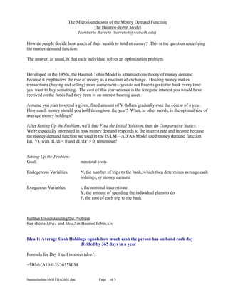
1. The Microfoundations of the Money Demand Function
The Baumol-Tobin Model
Humberto Barreto (barretoh@wabash.edu)
How do people decide how much of their wealth to hold as money? This is the question underlying
the money demand function.
The answer, as usual, is that each individual solves an optimization problem.
Developed in the 1950s, the Baumol-Tobin Model is a transactions theory of money demand
because it emphasizes the role of money as a medium of exchange. Holding money makes
transactions (buying and selling) more convenient—you do not have to go to the bank every time
you want to buy something. The cost of this convenience is the foregone interest you would have
received on the funds had they been in an interest bearing asset.
Assume you plan to spend a given, fixed amount of Y dollars gradually over the course of a year.
How much money should you hold throughout the year? What, in other words, is the optimal size of
average money holdings?
After Setting Up the Problem, we'll find Find the Initial Solution, then do Comparative Statics.
We're especially interested in how money demand responds to the interest rate and income because
the money demand function we used in the IS/LM—AD/AS Model used money demand function
L(i, Y), with dL/di < 0 and dL/dY > 0, remember?
Setting Up the Problem:
Goal: min total costs
Endogenous Variables: N, the number of trips to the bank, which then determines average cash
holdings, or money demand
Exogenous Variables: i, the nominal interest rate
Y, the amount of spending the individual plans to do
F, the cost of each trip to the bank
Further Understanding the Problem
See sheets Idea1 and Idea2 in BaumolTobin.xls
Idea 1: Average Cash Holdings equals how much cash the person has on hand each day
divided by 365 days in a year
Formula for Day 1 cell in sheet Idea1:
=$B$4-(A10-0.5)/365*$B$4
baumoltobin-160311162601.doc Page 1 of 5

2. Idea 2: Average Cash Holdings equals Y/2N
Idea 2B: This means that total foregone interest equals i x Y/2N
Set the Number of
Trips to the Bank
in Idea2 sheet.
So, as N increases, the cost of foregone interest falls AND the total cost of going to the bank rises.
The separate graphs look like this:
The Cost of Foregone Income depends on i, Y, and N, like this:
Y 10,000$ amount of dollars to be spent gradually ov er the y ear
i 10% interest rate per y ear
i x Y/2N
N Cost of f oregone income
1 500.00$
5 100.00$
73 6.85$
365 1.37$
Cost of Foregone Income
$-
$100.00
$200.00
$300.00
$400.00
$500.00
$600.00
0 100 200 300 400
N
The Cost of Going to the bank depends on F and N, like this:
F 5.00$ per unit cost of each trip to the bank
FN
N Cost of Going to the Bank
1 5.00$
5 25.00$
73 365.00$
365 1,825.00$
Costs of Going to the Bank
$-
$500.00
$1,000.00
$1,500.00
$2,000.00
0 100 200 300 400
N
The tension in the problem is easy to see. As N rises, the Cost of Foregone falls, but the Cost of
Going to the Bank rises. How many trips should be taken? The cost minimizing amount.
baumoltobin-160311162601.doc Page 2 of 5

3. Finding the Initial Solution:
• Graphically
That’s easy. Put the two graphs together. See Underlying Graph sheet.
The Total Cost is the sum of the two individual costs.
Y 10,000$ amount of dollars to be spent gradually ov er the y ear
i 10% interest rate, compounded daily so that i/365 is daily interest rate
F 5 cost per trip to the bank
i x Y/2N FN i x Y/2N + FN
N
Cost of
Foregone
Income
Cost of Going
to the Bank Total Cost
5 100.00$ 25.00$ 125.00$
7.5 66.67$ 37.50$ 104.17$
10 50.00$ 50.00$ 100.00$
12.5 40.00$ 62.50$ 102.50$
15 33.33$ 75.00$ 108.33$
17.5 28.57$ 87.50$ 116.07$
20 25.00$ 100.00$ 125.00$
Figure 18-2: The Cost of Holding Money
Cost of
Foregone
Interest
Cost of Going
to the Bank
Total
Cost
$-
$20.00
$40.00
$60.00
$80.00
$100.00
$120.00
$140.00
0 5 10 15 20 25
N
BaumolTobin.xls
• Excel’s Solver
See sheet Optimization in BaumolTobin.xls
Execute Tools: Solver. The Solver dialog box has been configured for you. The goal to Min Total
Costs in cell B6 by choosing N in cell B14, given the exogenous variables, Y, i, and F.
Excel's Solver gets very close, but not exactly equal to 1. That's a numerical algorithm for
you. When little is gained, it stops hunting for a better solution and announces that it has
converged to a solution.
You can tighten the convergence criterion by clicking on the Options button in the Solver
dialog box. Explore Convergence, Precision, and Tolerance.
baumoltobin-160311162601.doc Page 3 of 5

4. • Calculus
Here's the analytical solution.
min TC =
iY
2N
+ FN
dTC
dN
= −
iY
2N
2
+ F
At a min, this derivative is equal to zero, so
−
iY
2N
*2 + F = 0
iY
2F
= N
*2
N*
=
iY
2F
At i =10%,Y = $10,000, and F = $5/trip,
N*
=
0.10 * $10,000
2 *5
=10
Notice that N* is not money demand. Money demand is average cash holdings, M
d
=
Y
2N
, and
must be calculated like this:
Md*
=
Y
2
iY
2F
=
YF
2i
At i =10%, Y= $10,000, and F =$5/trip,
Md*
=
(10,000)*(5)
2*(0.1)
=$500
The equation for optimal money holding, M
d*
=
YF
2i
, is the money demand function, L(Y,i) that we
were trying to derive. Notice how it behaves as expected—increases in Y lead to increases in money
demand and increases in i lead to decreases in money demand.
• Comparing Excel and Calculus
Although Solver didn't give us exactly 1, for all intents and purposes we are getting the same answer
(as shown by the data in the Optimization sheet).
baumoltobin-160311162601.doc Page 4 of 5

5. Comparative Statics
There are three exogenous variables in the model and they all appear in the optimal money demand
equation. We can do comparative statics from the perspective of Y, i, and F.
In each case, we can proceed analytically, taking the derivative of the optimal money demand
function, or numerically, changing the exogenous variable by an arbitrary, finite amount and
recalculating the optimal solution. Of course, the Comparative Statics Wizard add-in makes the
latter approach much easier.
baumoltobin-160311162601.doc Page 5 of 5

6. Comparative Statics
There are three exogenous variables in the model and they all appear in the optimal money demand
equation. We can do comparative statics from the perspective of Y, i, and F.
In each case, we can proceed analytically, taking the derivative of the optimal money demand
function, or numerically, changing the exogenous variable by an arbitrary, finite amount and
recalculating the optimal solution. Of course, the Comparative Statics Wizard add-in makes the
latter approach much easier.
baumoltobin-160311162601.doc Page 5 of 5