Post

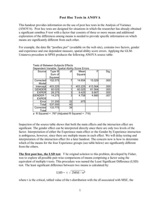
1. 1
Post Hoc Tests in ANOVA
This handout provides information on the use of post hoc tests in the Analysis of Variance
(ANOVA). Post hoc tests are designed for situations in which the researcher has already obtained
a significant omnibus F-test with a factor that consists of three or more means and additional
exploration of the differences among means is needed to provide specific information on which
means are significantly different from each other.
For example, the data file “posthoc.por” (available on the web site), contains two factors, gender
and experience and one dependent measure, spatial ability score errors. Applying the GLM-
Unianova procedure in SPSS produces the following ANOVA source table:
Tests of Between-Subjects Effects
Dependent Variable: Spatial Ability Score Errors
Source Type III
Sum of
Squares
df Mean
Square
F Sig.
Corrected
Model
102.575 7 14.654 15.029 .000
Intercept 403.225 1 403.225 413.564 .000
GENDER 60.025 1 60.025 61.564 .000
EXPER 28.275 3 9.425 9.667 .000
GENDER *
EXPER
14.275 3 4.758 4.880 .007
Error 31.200 32 .975
Total 537.000 40
Corrected
Total
133.775 39
a R Squared = .767 (Adjusted R Squared = .716)
Inspection of the source table shows that both the main effects and the interaction effect are
significant. The gender effect can be interpreted directly since there are only two levels of the
factor. Interpretation of either the Experience main effect or the Gender by Experience interaction
is ambiguous, however, since there are multiple means in each effect. We will delay testing and
interpretation of the interaction effect for a later handout. The concern now is how to determine
which of the means for the four Experience groups (see table below) are significantly different
from the others.
The first post hoc, the LSD test. T he original solution to this problem, developed by Fisher,
was to explore all possible pair-wise comparisons of means comprising a factor using the
equivalent of multiple t-tests. This procedure was named the Least Significant Difference (LSD)
test. The least significant difference between two means is calculated by:
_________
LSD = t o 2MSE / n*
where t is the critical, tabled value of the t-distribution with the df associated with MSE, the

2. 2
denominator of the F statistic and n* is the number of scores used to calculate the means of
criticalinterest. In our example, t at " = .05, two-tailed, with df = 32 is 2.0369, MSE from the
source table above is 0.975, and n* is 10 scores per mean.
_________ __________
LSD = t o 2MSE / n* = 2.0369 o 2 (.975 / 10 = 0.6360
So the LSD or minimum difference between a pair of means necessary for statistical significance is
0.636.
In order to compare this critical value or difference for all our means it is useful to organize the
means in a table. First, the number of pair-wise comparisons among means can be calculated using
the formula: k(k-1)/2, where k = the number of means or levels of the factor being tested. In our
present example, the experience factor has four levels so k = 4 and there are k(k-1)/2 = 4(3)/2 = 6
unique pairs of means that can be compared.
Experience with Mechanical Problems
Dependent Variable: Spatial Ability Score Errors
Mean Std. Error 95%
Confidence
Interval
Experience Lower Bound Upper Bound
A lot 2.100 .312 1.464 2.736
Fair Amount 2.700 .312 2.064 3.336
Some 3.600 .312 2.964 4.236
Little to none 4.300 .312 3.664 4.936
The table we will construct is a table showing the obtained means on the rows and columns and
subtracted differences between each pair of means in the interior cells producing a table of
absolute mean differences to use in evaluating the post hoc tests. To construct the table follow
these steps: 1) rank the means from largest to smallest, 2) create table rows beginning with the
largest mean and going through the next-to-smallest mean, 3) create table columns starting with
the smallest mean and going through the next-to-largest mean, 4) compute the absolute difference
between each row and column intersection/mean. In the present example this results in the table of
absolute mean differences below:
2.1 2.7 3.6
4.3 2.2 1.6 0.7
3.6 1.5 0.9
2.7 0.6
Now applying our LSD value of .636 to the mean differences in the table, it can be seen that all
differences among the means are significant at " = .05 except the last difference between the

3. 3
means of 2.1 and 2.7. Unfortunately, the p-values associated with these multiple LSD tests are
inaccurate. Since the sampling distribution for t assumes only one t-test from any given sample,
substantial alpha slippage has occurred because 6 tests have been performed on the same sample.
The true alpha level given multiple tests or comparisons can be estimated as 1 - (1 - " ) , where c
c
= the total number of comparisons, contrasts, or tests performed. In the present example
1 - (1 - " ) = 1 - (1 - .05) = .2649. Given multiple testing in this situation, the true value of
c 6
alpha is approximately .26 rather than .05.
A number of different solutions and corrections have been developed to deal with this problem
and produce post hoc tests that correct for multiple tests so that a correct alpha level is
maintained even though multiple tests or comparisons are computed. Several of these approaches
are discussed below.
Tukey’s HSD test. Tukey’s test was developed in reaction to the LSD test and studies have
shown the procedure accurately maintains alpha levels at their intended values as long as
statistical model assumptions are met (i.e., normality, homogeneity, independence). Tukey’s HSD
was designed for a situation with equal sample sizes per group, but can be adapted to unequal
sample sizes as well (the simplest adaptation uses the harmonic mean of n-sizes as n*). The
formula for Tukey’s is:
_________
HSD = q o MSE / n*
where q = the relevant critical value of the studentized range statistic and n* is the number of
scores used in calculating the group means of interest. Calculation of Tukey’s for the present
example produces the following:
_________ ________
HSD = q o MSE / n* = 3.83 o .975 / 10 = 1.1957
The q value of 3.83 is obtained by reference to the studentized range statistic table looking up the
q value for an alpha of .05, df = < = 32, k = p = r = 4. Thus the differences in the table of mean
differences below that are marked by the asterisks exceed the HSD critical difference and are
significant at p < .05. Note that two differences significant with LSD are now not significant.
2.1 2.7 3.6
4.3 2.2* 1.6* 0.7
3.6 1.5* 0.9
2.7 0.6
Scheffe’s test. Scheffe’s procedure is perhaps the most popular of the post hoc procedures, the
most flexible, and the most conservative. Scheffe’s procedure corrects alpha for all pair-wise or
simple comparisons of means, but also for all complex comparisons of means as well. Complex
comparisons involve contrasts of more than two means at a time. As a result, Scheffe’s is also the

4. 4
least statistically powerful procedure. Scheffe’s is presented and calculated below for our pair-
wise situation for purposes of comparison and because Scheffe’s is commonly applied in this
situation, but it should be recognized that Scheffe’s is a poor choice of procedures unless complex
comparisons are being made.
For pair-wise comparisons, Scheffe’s can be computed as follows:
critical 1 2o(k -1) F oMSE (1/n + 1/n )
In our example:
o(3)(2.9011) o .975 (.1 + .1) = 2.9501 = 1.3027
And referring to the table of mean differences above, it can be seen that, despite the more
stringent critical difference for Scheffe’s test, in this particular example, the same mean differences
are significant as found using Tukey’s procedure.
Other post hoc procedures. A number of other post hoc procedures are available. There is a
Tukey-Kramer procedure designed for the situation in which n-sizes are not equal. Brown-
Forsythe’s post hoc procedure is a modification of the Scheffe test for situations with
heterogeneity of variance. Duncan’s Multiple Range test and the Newman-Keuls test provide
different critical difference values for particular comparisons of means depending on how adjacent
the means are. Both tests have been criticized for not providing sufficient protection against alpha
slippage and should probably be avoided. Further information on these tests and related issues in
contrast or multiple comparison tests is available from Kirk (1982) or Winer, Brown, and Michels
(1991).
Comparison of three post hoc tests. As should be apparent from the foregoing discussion, there
are substantial differences among post hoc procedures. The procedures differ in the amount and
kind of adjustment to alpha provided. The impact of these differences can be seen in the table of
critical values for the present example shown below:
Critical Difference
LSD 0.6360
Tukey 1.1957
Scheffe 1.3027
The most important issue is to choose a procedure which properly and reliably adjusts for the
types of problems encountered in your particular research application. Although Scheffe’s
procedure is the most popular due to its conservatism, it is actually wasteful of statistical power
and likely to lead to Type II errors unless complex comparisons are being made. When all pairs of
means are being compared, Tukey’s is the procedure of choice. In special design situations, other
post hoc procedures may also be preferable and should be explored as alternatives.
© Stevens, 1999