Radio pulsars scintillate because their emission travels through the ionized interstellar medium along multiple paths, which interfere with each other. It has long been realized that, independent of their nature, the regions responsible for the scintillation could be used as ‘interstellar lenses’ to localize pulsar emission regions1,2 . Most such lenses, however, resolve emission components only marginally, limiting results to statistical inferences and detections of small positional shifts3–5 . As lenses situated close to their source offer better resolution, it should be easier to resolve emission regions of pulsars located in high-density environments such as supernova remnants6 or binaries in which the pulsar’s companion has an ionized outflow. Here we report observations of extreme plasma lensing in the ‘black widow’ pulsar, B1957+20, near the phase in its 9.2-hour orbit at which its emission is eclipsed by its companion’s outflow7–9 . During the lensing events, the observed radio flux is enhanced by factors of up to 70–80 at specific frequencies. The strongest events clearly resolve the emission regions: they affect the narrow main pulse and parts of the wider interpulse differently. We show that the events arise naturally from density fluctuations in the outer regions of the outflow, and we infer a resolution of our lenses that is comparable to the pulsar’s radius, about 10 kilometres. Furthermore, the distinct frequency structures imparted by the lensing are reminiscent of what is observed for the repeating fast radio burst FRB 121102, providing observational support for the idea that this source is observed through, and thus at times strongly magnified by, plasma lenses10

1. Letter https://doi.org/10.1038/s41586-018-0133-z
Pulsar emission amplified and resolved by plasma
lensing in an eclipsing binary
Robert Main1,2,3
*, I-Sheng Yang3,4
, Victor Chan1
, Dongzi Li3,5
, Fang Xi Lin3,5
, Nikhil Mahajan1
, Ue-Li Pen3,6,2,4
,
Keith Vanderlinde1,2
& Marten H. van Kerkwijk1
Radio pulsars scintillate because their emission travels through the
ionized interstellar medium along multiple paths, which interfere
with each other. It has long been realized that, independent of their
nature, the regions responsible for the scintillation could be used
as ‘interstellar lenses’ to localize pulsar emission regions1,2
. Most
such lenses, however, resolve emission components only marginally,
limiting results to statistical inferences and detections of small
positional shifts3–5
. As lenses situated close to their source offer
better resolution, it should be easier to resolve emission regions of
pulsars located in high-density environments such as supernova
remnants6
or binaries in which the pulsar’s companion has an
ionized outflow. Here we report observations of extreme plasma
lensing in the ‘black widow’ pulsar, B1957+20, near the phase in its
9.2-hour orbit at which its emission is eclipsed by its companion’s
outflow7–9
. During the lensing events, the observed radio flux is
enhanced by factors of up to 70–80 at specific frequencies. The
strongest events clearly resolve the emission regions: they affect the
narrow main pulse and parts of the wider interpulse differently. We
show that the events arise naturally from density fluctuations in
the outer regions of the outflow, and we infer a resolution of our
lenses that is comparable to the pulsar’s radius, about 10 kilometres.
Furthermore, the distinct frequency structures imparted by the
lensing are reminiscent of what is observed for the repeating fast
radio burst FRB 121102, providing observational support for the
idea that this source is observed through, and thus at times strongly
magnified by, plasma lenses10
.
On 2014 June 13–16, we took 9.5 h of data of PSR B1957+20 with
the 305-m William E. Gordon Telescope at the Arecibo observatory, at
observing frequency of 311.25–359.25 MHz (see Methods). These data
were previously searched for giant pulses11
—sporadically occurring,
extremely bright pulses, which are much shorter than regular pulses
(around 1 μs compared with tens of microseconds). Although we found
many giant pulses at all orbital phases, we noticed that the incidence
rate of bright pulses was much higher leading up to and following the
radio eclipse.
As can be seen in Fig. 1, most of the pulses near eclipse do not look
like giant pulses but rather like brighter regular pulses—they are bright
over a large fraction of the pulse profile, and most tellingly, occur in
groups spanning several 1.6-ms pulse rotations, suggesting that the
underlying events last for a time of the order of 10 ms. Their proper-
ties seem similar to the hitherto mysterious bright pulses associated
with the eclipse of PSR J1748 − 2446A12
, suggesting a shared physical
mechanism.
High-magnification events are often chromatic, as can be seen from
the colours in Fig. 1 (which reflect 16-MHz sub-bands) and is borne
out more clearly by the spectra shown in Fig. 2: some show frequency
widths comparable to our 48-MHz band, peaking at low or high fre-
quency, whereas others show strong frequency evolution, in some cases
tracing out a slope in frequency–time space, in others a double-peaked
profile.
For many high-magnification events, the magnification is not
uniform across the pulse profile. The bottom panel of Fig. 1 shows this
strikingly: at 0.2 s, the main pulse is greatly magnified over five pulses,
whereas the entire interpulse is barely affected. In addition, the compo-
nents of the broad interpulse are often magnified differently from each
other, as can be seen most readily in the magnified events in Fig. 3b, c.
Thus, the events resolve the pulsar’s various emission regions.
The most strongly magnified events occur within three specific time
spans, each lasting for about 5 min, around orbital phase φ = 0.20,
φ = 0.30 and φ = 0.32 (see Fig. 1); here, φ = 0.25 corresponds to supe-
rior conjunction of the pulsar in its 9.2-h orbit7
, and the duration of
the eclipses at 350 MHz is about 40 to 60 min (refs. 7–9
), or ∆φ ≈ 0.1
(a sketch of the system geometry is shown in Extended Data Fig. 1). In
each time span, we observe only small overall frequency-dependent
time delays, of the order of 10 μs, which indicate modest increases
in electron column density, with dispersion measures of the order of
10−4
pc cm−3
(see Fig. 1 as well as Extended Data Fig. 2). Intriguingly,
at times when the delays are longer and the dispersion measures thus
higher—immediately before and after eclipse, and in between the two
post-eclipse periods of strong lensing, at φ ≈ 0.31—the magnifica-
tions are less marked, only up to a factor of a few, and correlated over
much longer timescales, of the order of 100 ms. After the main lensing
periods, up to φ ≈ 0.36, flux variations remain correlated, suggesting
that even weaker events are still present (examples of lensing in the
aforementioned regions are shown in Extended Data Fig. 3).
To determine whether the magnification events could be due to lens-
ing by inhomogeneities in the companion’s outflow, we first measured the
excess delay due to dispersion at a time resolution of 2 s, the shortest at
which we can measure it reliably (see Methods). We find that during the
periods of strong magnification events, the delay fluctuates by about 1 μs
on this timescale. Assuming that the relative velocity between the pulsar
and the companion’s outflow is roughly the orbital velocity, 360 km s−1
(ref. 13
), the 2-s timescale corresponds to a spatial scale ∆x ≈ 720 km.
For this scale, the expected geometric delay is ∆x2
/2ac ≈ 0.5 μs (where
a = 6.4 light-seconds is the orbital separation and c the speed of light). As
this is comparable to the observed dispersive delays, lensing is expected.
To model the magnified pulses, we treat the signal using a standard
wave-optics formalism. The electric field received by an observer is the
sum of the electric field of the source across the lens plane, with the
phase at every point determined by both geometric and dispersive
delays. When a large area on the plane has (nearly) stationary phase,
the electric field combines coherently, leading to a strongly magnified
image, with the magnification μ proportional to the area squared.
Because dispersive and geometric delays scale differently with fre-
quency ν, a plasma lens cannot be in focus over all frequencies, but will
impart a characteristic frequency width. This width will be smaller for
larger magnification, with the precise scaling depending on the extent
to which the lens is elliptic: Δν/ν ~ 1/μ for a very elongated, effectively
linear lens, and ν ν μΔ / ~ /1 for a (roughly) circular one. In strong
lensing, one generically expects multiple images to contribute, and thus
1
Department of Astronomy and Astrophysics, University of Toronto, Toronto, ON, Canada. 2
Dunlap Institute for Astronomy and Astrophysics, University of Toronto, Toronto, ON, Canada. 3
Canadian
Institute for Theoretical Astrophysics, University of Toronto, Toronto, ON, Canada. 4
Perimeter Institute for Theoretical Physics, Waterloo, ON, Canada. 5
Department of Physics, University of Toronto,
Toronto, ON, Canada. 6
Canadian Institute for Advanced Research, Toronto, ON, Canada. *e-mail: main@astro.utoronto.ca
5 2 2 | N A T U RE | V O L 5 5 7 | 2 4 M A Y 2 0 1 8
© 2018 Macmillan Publishers Limited, part of Springer Nature. All rights reserved.

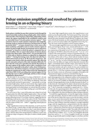
2. Letter RESEARCH
caustics to form, which can lead to a slope in time–frequency space,
double-peaked spectra and other interference effects (see Methods).
All of these are consistent with the behaviour seen in the measured
spectra of the magnified pulses in Fig. 2.
For any lens, different pulse components will be magnified differently
if they arise from regions that have projected separations larger than
the lens’s resolution. We can make a quantitative estimate of the lens
resolution by using the magnifications of the events. Continuing to
assume the lens is roughly co-located with the companion, that is, at
the orbital separation a, the resolution of the lens for given magnifica-
tion would be ≈ 1.9R1/μ1/2
for a linear lens, or ≈ 1.9R1/μ1/4
for a circu-
lar one, where λ≡ /πR a1 , or 23 km at our observing wavelength
λ ν= / ≈c 90cm (see Methods for a derivation). A peak magnification
of, for instance, μ = 50 then corresponds to a physical resolution of
about 6 km for a linear lens or about 17 km for a circular one.
The inferred resolution is comparable to the radius (approximately
10 km) of the neutron star, and substantially smaller than the light-
cylinder radius, RLC ≡ cP/2π = 76 km, where the velocity of co-
rotating magnetic fields approaches the speed of light, bounding
the magnetosphere in which pulsar emission is thought to origi-
nate14
. Thus, the lensing offers the opportunity to map the emission
geometry.
Qualitatively, because the main pulse and interpulse, as well as parts
of the wide interpulse beam, are sometimes magnified very differently,
the inferred resolution is a lower limit both to the projected separation
between the main pulse and the interpulse, and to the size of the inter-
pulse. Perhaps not unexpectedly, the spatial separations do not seem to
map directly to rotational phase: we see similar differences between the
main pulse and the interpulse, which are separated by half a rotation,
and between parts of the interpulse, which are separated by only about
0.1 rotation. This may indicate that the interpulse consists of multiple
components, which are not located close together in space.
Combining the lens resolution with the timescale of the lensing
events allows us to constrain the projected relative velocity between the
lens and the pulsar. A priori, one might expect the outflow velocity to be
slow, in which case the relative velocity would just be the orbital motion
of about 360 km s−1
. Given that strong magnification events typically
last about 10 ms, this would then imply a resolution of approximately
Fig. 1 | Strong lensing of the pulsar. a, Magnification distributions for the
main pulse, in 10-s time bins, showing periods of lensing near ingress and
egress of the eclipse of the pulsar by its companion’s outflow. The greyscale
is logarithmic, to help individual bright pulses to stand out. b, Pulse
profiles as a function of time, averaged over 10 s and in 128 phase bins.
Cyan, yellow and magenta represent contiguous 16-MHz sub-bands, from
low to high frequency. Near eclipse, plasma dispersion causes frequency-
dependent delays. Gaps in the data correspond to calibrator scans.
c, d, Enlargements in which each time bin corresponds to an individual
1.6-ms pulse. One sees extreme chromatic lensing in which pulses
are magnified by an order of magnitude over tens of milliseconds; the
brightest event is magnified by a factor of about 40 across our highest-
frequency sub-band. In some events, the main pulse and interpulse are
clearly affected differently, indicating that different emission regions
corresponding to these are resolved by the lensing structures.
e, f, Enlargements for a quiescent period for comparison.
0 1,800 3,600 5400
0.0
0.5
1.0
b
0 1 2
0.0
0.5
1.0
Rotationalphase
c
0.0 0.1 0.2
Time (s)
0.0
0.5
1.0
d
0 1
e
0.0 0.1
f
0
20
40
Magnification
0.20 0.25 0.30 0.35 0.40 0.45
Orbital phase
a
7,200
2 4 M A Y 2 0 1 8 | V O L 5 5 7 | N A T U RE | 5 2 3
© 2018 Macmillan Publishers Limited, part of Springer Nature. All rights reserved.

3. LetterRESEARCH
4 km, not dissimilar from what we find above, thus suggesting that
the assumption of a slow outflow velocity is reasonable. By combining
different constraints between the duration and frequency widths of
lensing events, we can set a quantitative limit to the relative velocity
(see Methods for a derivation), of
ν
ν
> .
Δ



Δ 


>
/
−
v
R
t
0 5 360 kms (1)1
HWHM HWHM
1 2
1
where for the numerical value we use the fact that the tightest con-
straints come from the shortest, least chromatic events, which have
frequency widths ν νΔ / ≈ .( ) 0 1HWHM
, and durationsΔ ≈t 10msHWHM
(measured as half-width at half-maximum, HWHM; see Fig. 2). This
approximate limit equals the relative orbital velocity, which implies that
the outflow velocity can be (but does not have to be) small in the rest
frame of the companion.
Our results offer many avenues of further research. Ideally, one
would use the lensing to map the pulsar magnetosphere. This requires
better constraints on the lenses, for example from observations over
several eclipses at a range of frequencies. Further observations may
also shed light on the eclipse mechanism. For example, if it is cyc-
lo-synchrotron absorption, large magnetic fields, of about 20 G, are
required15
, which would impart measurable polarization dependence
of the lensing events. Furthermore, combining density and velocity into
0
10
320
335
350
0 30
0
30
0 60
0
20
320
335
350
0 30
0
10
0 20
0
5
320
335
350
0 20
0
10
0 20
0
5
−40 −20 0 20 40
Pulse number
320
335
350
0 10
0
5
−40 −20 0 20 40
Pulse number
0 10
Observingfrequency(MHz)andmagnification
Fig. 2 | A range of spectral behaviour in lensing events. Power spectra,
binned to 3 MHz, of the main pulse in consecutive 1.6-ms rotations, for
selected lensing events from eclipse egress. The top panels show the average
magnification in each main pulse, and the side panels the magnification
spectra of the brightest pulse (that is, that of pulse number 0).
aa
×50
–5
0
5
bb
–5
0
5
Pulsenumber
cc
0.0 0.2 0.4 0.6 0.8 1.0
Rotational phase
–5
0
5
dd
Fig. 3 | Profiles of lensing events. a, Frequency-averaged pulse profile
of a 9-min quiescent region, scaled up by a factor of 50 for comparison
purposes; b, c, d, frequency-averaged pulse profiles surrounding bright
events (using 128 phase bins). One sees that the events resolve the
magnetosphere: the main pulse and interpulse are affected differently, as
are parts within the interpulse.
5 2 4 | N A T U RE | V O L 5 5 7 | 2 4 M A Y 2 0 1 8
© 2018 Macmillan Publishers Limited, part of Springer Nature. All rights reserved.

4. Letter RESEARCH
a mass-loss rate of the outflow, one can infer the lifetime, and thus the
final fate, of these systems.
Finally, our observations establish that radio pulses can be strongly
amplified by lensing in local ionized material. This adds support
for the proposal that fast radio bursts (FRBs) can be lensed by
host galaxy plasma, leading to variable magnification, narrow
frequency structures and clustered arrival times of highly amplified
(and thus observable) events10
. Evidence for high-density environ-
ments includes that FRB 110523 is scattered within its host galaxy16
,
and that FRB 121102 has been localized to a star-forming region17,18
,
in an extreme and dynamic magneto-ionic environment19
. Indeed,
the latter’s repeating bursts have spectra20–22
remarkably similar to
those shown in Fig. 2 (for example, compare with Fig. 2 of ref. 20
),
and, like those bursts, the brightest pulses in PSR B1957+20 are highly
clustered in time.
Online content
Any Methods, including any statements of data availability and Nature Research
reporting summaries, along with any additional references and Source Data files,
are available in the online version of the paper at https://doi.org/10.1038/s41586-
018-0133-z.
Received: 7 December 2017;Accepted: 5 March 2018;
Published online 23 May 2018.
1. Lovelace, R. V. E. Theory and Analysis of Interplanetary Scintillations. PhD thesis,
Cornell Univ. (1970).
2. Backer, D. C. Interstellar scattering of pulsar radiation. I: Scintillation. Astron.
Astrophys. 43, 395–404 (1975).
3. Gwinn, C. R. et al. Size of the Vela pulsar’s emission region at 18 cm wavelength.
Astrophys. J. 758, 7 (2012).
4. Johnson, M. D., Gwinn, C. R. & Demorest, P. Constraining the Vela pulsar’s radio
emission region using Nyquist-limited scintillation statistics. Astrophys. J. 758, 8
(2012).
5. Pen, U.-L., Macquart, J.-P., Deller, A. T. & Brisken, W. 50 picoarcsec astrometry of
pulsar emission. Mon. Not. R. Astron. Soc. 440, L36–L40 (2014).
6. Main, R. et al. Mapping the emission location of the Crab pulsar’s giant pulses.
Preprint at https://arxiv.org/abs/1709.09179 (2017).
7. Fruchter, A. S., Stinebring, D. R. & Taylor, J. H. A millisecond pulsar in an
eclipsing binary. Nature 333, 237–239 (1988).
8. Fruchter, A. S. et al. The eclipsing millisecond pulsar PSR 1957 + 20. Astrophys.
J. 351, 642–650 (1990).
9. Ryba, M. F. & Taylor, J. H. High-precision timing of millisecond pulsars. II:
Astrometry, orbital evolution, and eclipses of PSR 1957 + 20. Astrophys. J. 380,
557–563 (1991).
10. Cordes, J. M. et al. Lensing of fast radio bursts by plasma structures in host
galaxies. Astrophys. J. 842, 35 (2017).
11. Main, R., van Kerkwijk, M., Pen, U.-L., Mahajan, N. & Vanderlinde, K. Descattering
of giant pulses in PSR B1957+20. Astrophys. J. Lett. 840, L15 (2017).
12. Bilous, A. V., Ransom, S. M. & Nice, D. J. in American Institute of Physics Conf. Ser.
Vol. 1357 (eds Burgay, M. et al.) 140–141 (2011).
13. Van Kerkwijk, M. H., Breton, R. P. & Kulkarni, S. R. Evidence for a massive
neutron star from a radial-velocity study of the companion to the black-widow
pulsar PSR B1957+20. Astrophys. J. 728, 95 (2011).
14. Ginzburg, V. L. & Zhelezniakov, V. V. On the pulsar emission mechanisms. Annu.
Rev. Astron. Astrophys. 13, 511–535 (1975).
15. Thompson, C., Blandford, R. D., Evans, C. R. & Phinney, E. S. Physical processes
in eclipsing pulsars: eclipse mechanisms and diagnostics. Astrophys. J. 422,
304–335 (1994).
16. Masui, K. et al. Dense magnetized plasma associated with a fast radio burst.
Nature 528, 523–525 (2015).
17. Tendulkar, S. P. et al. The host galaxy and redshift of the repeating fast radio
burst FRB 121102. Astrophys. J. Lett. 834, L7 (2017).
18. Bassa, C. G. et al. FRB 121102 is coincident with a star-forming region in its
host galaxy. Astrophys. J. Lett. 843, L8 (2017).
19. Michilli, D. et al. An extreme magneto-ionic environment associated with the
fast radio burst source FRB 121102. Nature 553, 182–185 (2018).
20. Spitler, L. G. et al. A repeating fast radio burst. Nature 531, 202–205 (2016).
21. Scholz, P. et al. The repeating fast radio burst FRB 121102: multi-wavelength
observations and additional bursts. Astrophys. J. 833, 177 (2016).
22. Law, C. J. et al. A multi-telescope campaign on FRB 121102: implications for
the FRB population. Astrophys. J. 850, 76 (2017).
Acknowledgements We thank A. Bilous for sharing and discussing her results
which motivated this analysis. We thank the rest of our scintillometry group for
discussions and support throughout. R.M., M.H.v.K., U.-L.P. and K.V. are funded
through NSERC. I-S.Y was supported by a SOSCIP Consortium Postdoctoral
Fellowship.
Reviewer information Nature thanks S. Ransom and J. Hessels for their
contribution to the peer review of this work.
Author contributions R.M. discovered the magnified pulses; wrote the majority
of the manuscript; and created the figures. I-S.Y. developed and wrote the
sections on wave-optics formalism in the Methods; M.H.v.K and U.-L.P. guided
the analysis and interpretation of the results; M.H.v.K. also helped to write
the manuscript and influenced the content and presentation of the figures;
F.X.L., V.C. and K.V. quantified the excess dispersion measure associated with
the eclipse. N.M. wrote the code used to produce the coherently de-dispersed
single pulse profiles used in this analysis, and derived an improved orbital
ephemeris relative to which time delays are measured. D.L. worked on criteria to
systematically separate giant pulses from pulses magnified by plasma lensing.
All authors contributed to the interpretation of results.
Competing interests The authors declare no competing financial interests.
Additional information
Extended data is available for this paper at https://doi.org/10.1038/s41586-
018-0133-z.
Reprints and permissions information is available at http://www.nature.com/
reprints.
Correspondence and requests for materials should be addressed to R.M.
Publisher’s note: Springer Nature remains neutral with regard to jurisdictional
claims in published maps and institutional affiliations.
2 4 M A Y 2 0 1 8 | V O L 5 5 7 | N A T U RE | 5 2 5
© 2018 Macmillan Publishers Limited, part of Springer Nature. All rights reserved.

5. LetterRESEARCH
Methods
Calculating magnifications. The data were taken in four 2.4-h sessions on 2014
June 13–16 and were recorded as part of a European VLBI network programme
(GP 052). The data span 311.25–359.25 MHz, in three contiguous 16-MHz sub-
bands, and we read, de-dispersed (with a dispersion measure of 29.1162 pc cm−3
)
and reduced the data as described in ref. 11
. As one extra step, we accounted for
the wander in orbital period of PSR B1957+20 by adjusting the time of ascending
node in the ephemeris, such that it minimized the scatter of the arrival times of
giant pulses associated with the main pulse across all four days of observation.
We define the magnification of a pulse as the ratio of its flux to the mean flux in
a quiescent region far from eclipse. Specifically, we construct an intensity profile of
each pulse using 128 phase gates, subtract the mean off-pulse flux in each 16-MHz
sub-band separately, measure the flux in an eight-gate (approximately 100 μs)
window around the peak location (which we find from folded profiles, averaged in
2-s bins to obtain sufficient signal-to-noise), and divide by the average flux in the
same pulse window measured in a 9-min section far from eclipse.
To construct the spectra of lensing events, we start by binning power spectra in
3-MHz bins. We correct these approximately for the bandpass and the effects of
interstellar scintillation (which still has a small amount of power on 3-MHz scales)
by dividing them by the average spectra in the 15 s before and after (excluding the
lensing event itself). This time span is chosen to be safely less than the timescale
of about 84 s on which the interstellar scintillation pattern varies11
, ensuring the
dynamic spectrum is stable on these scales. With 30 s of data, it is also very well
measured: each 3-MHz channel has signal-to-noise ratio S/N ≈ 150.
Evidence that strong plasma lensing must occur. To obtain the properties of the
lensed images, and in particular to determine whether we are in the ‘strong’ or
‘weak’ lensing regime—that is, whether or not multiple images are formed—we use
the basic principles of wave optics, considering path integrals of the electric field
over a thin lens23
. In our case, the phase of an electromagnetic wave going through
different paths has contributions from both geometric and dispersive time delays,
φ φ φ= +x y x y x y( , ) ( , ) ( , ) (2)GM DM
where x and y are in the lens plane. For a geometrically thin lens, that is, with
thickness along the line of sight much smaller than the separation a, the geometric
contribution to the phase can be written as
φ
λ
=



+ 








=
+x y
a
a x y
R
1
2 2
(3)GM
2 2
2
2 2
Fr
2
where RFr is the Fresnel scale,
λ≡ ≈R a 40 km (4)Fr
with λ the wavelength of the radiation. For the numerical value, we used λ =
c/ν = 90 cm (where ν is the observing frequency) and assumed that the lensing
material was associated with the companion and thus at the orbital separation of
a ≈ 6.4 light-seconds. (Note that as we are using wavelengths and frequencies of
full cycles, our phases are in cycles too, not radians.)
The dispersive contribution arises from the signal propagating through the lens’s
extra dispersion measure (electron column density) ∫Δ = n zDM de (with ne the
electron number density),
φ
ν
= − Δx y
k
x y( , ) DM( , ) (5)DM
DM
where kDM = e2
/2πmec = 4,148.808 s pc−1
cm3
MHz2
(ref. 24
). The minus sign arises
because in a plasma the phase velocity is greater than the speed of light.
Integrating over different paths, one effectively select regions where the electric
fields are coherent; these lead to the final images. For instance, if the extra electrons
are distributed uniformly (in the x–y plane after the z integral), then φDM is approx-
imately constant and the total phase has a stationary point around x = y = 0, that
is, around the line of sight. Furthermore, all paths that are less than the Fresnel
scale away from this central path have similar phase, and thus one recovers the
general result that the area of the lens that contributes scales with RFr
2 .
For the lensing to be strong, a minimum requirement is that changes in the
geometric and dispersive phase are of similar magnitude. Because dispersion also
leads to overall time delays, differences in pulse arrival time give a measure of
inhomogeneities in the lensing material. We measure pulse arrival times using
the usual procedure of fitting pulse profiles to a high signal-to-noise template
(from a quiescent period). We fit profiles in the three bands separately and con-
vert the weighted average to ΔDM using standard equations. We find that the
inferred ΔDM shows both the expected large-scale variations7
and considerable
variability down to the shortest timescales (2 s) at which we can measure it reliably
(see Extended Data Fig. 2). During the periods in which the strongly magni-
fied events occur, we find intrinsic variability corresponding to variations in
delay of ∆tDM ≈ 1 μs, which suggests that the inhomogeneities correspond
to differences in the dispersion phase of ΔφDM = νΔtDM ≈ 300 cycles at 2-s
timescales.
To compare this to the geometric phase, we need to translate the timescale
of 2 s to a length scale. Assuming the relative motion between the pulsar and
the lensing material is dominated by the orbital motion, of 360 km s−1
, the spatial
scale is 720 km. Using equation (3), this corresponds to ΔφGM (720 km) ≈ 200
cycles.
The fact that ΔφDM is comparable to and slightly larger than ΔφGM at the dis-
tance scale of 720 km guarantees that somewhere around this scale, slopes in φDM
and φGM will sometimes cancel. It also implies that multiple stationary points with
∇φ = 0 are likely. Because the phases result from a continuous function of x, y and
ν, the stationary points must emerge or annihilate in pairs, leading to so-called
caustics, where one has not just ∇φ = 0 but also det(∂i∂jφ) = 0 (ref. 25
).
Given the above, strong lensing is a natural cause of the strongly magnified
events that we observe.
A perfect lens model. To calculate properties of the lensed images, we would
need to perform the path integral. This is not possible, as it requires the value of
φDM of the full two-dimensional lens plane at a resolution better than the Fresnel
scale, whereas our time-delay measurements are limited to the one-dimensional
trajectory of the pulsar, and to an order of magnitude larger scales.
Hence, for our analysis we use a simplified model, amenable to wave-optics
analysis, in which each strong lensing event is associated with an elliptical perfect
lens, that is, there is a single focal point to which all paths within the lens contrib-
ute perfectly coherently, and all paths outside the lens do not contribute at all.
As shown in Extended Data Fig. 4, our model is parametrized by the location of
the focal point relative to the centre of the lens, (X, Y), the semi-major and semi-
minor axes of the lens, (Δxlens, Δylens) and the orientation relative to the projected
pulsar trajectory.
In the special case of a centred circular lens with radius R, that is, Δxlens = Δylens
= R and X = Y = 0, the set-up would produce an Airy disk. By comparing this to
the actual path-integral of an unlensed image (that is, with φDM = 0), we can
identify the unlensed case with a circular lens with radius π≡ /R R1 Fr .
Integrating the electric field over an elliptical lens, the magnification (defined
as the increase in intensity μ = I/〈I〉, where I = E2
), will be proportional to the
area squared:
μ
∆ ∆
=












x
R
y
R
(6)lens
1
2
lens
1
2
Before continuing, we note that at first glance it might seem puzzling for the
magnification to be proportional to image area squared, as that seems to violate
energy (flux) conservation. However, the image is also more highly beamed; what
we calculated is the magnification in the centre of the beam. Viewed from an angle,
a linear phase term is induced across the originally coherent region. Thus, when
the region is larger, it is easier to become incoherent. The solid angle scales as
ΩΔ ∝ Δ Δ− −
x ylens
1
lens
1
, and thus total energy (flux) is indeed proportional to the area
of the lens.
Differential magnification and chromaticity. We now proceed to derive the phys-
ical resolution of the lens. The above magnification is reached only when the source
is exactly at the focal point. When the emission region is some distance away from
the focal point, paths from it to different parts of elliptical region will have extra
phase differences. For instance, when a source is separated from the focal point in
the x direction by xsource ≡ (X − xs) (where xs is measured relative to the centre of
the lens), there is a phase difference across the lens of
φΔ =
Δx x
R
(7)
lens source
1
2
When this phase difference reaches order 1, the image from the new source loca-
tion will no longer be magnified. Defining the resolution as the offset for which
total cancellation happens, we find from an explicit integral over the elliptical lens1
∆
≈
.
x
R
x
1 9
(8)res
1
2
lens
∆
≈
.
y
R
y
1 9
(9)res
1
2
lens
Hence, total cancellation occurs on an elliptical beam with semi-minor and
semi-major axes xres and yres that scale inversely to the semi-major and semi-
minor axes of the lens.
© 2018 Macmillan Publishers Limited, part of Springer Nature. All rights reserved.

6. Letter RESEARCH
We can write the above in terms of the magnification for a specific lens model.
We will consider two extremes, the first a very anisotropic lens, effectively one-
dimensional, for which Δylens = R1. For this case,
μ
≈
.
/
x
R1 9
(10)res
1
1 2
In the opposite direction, we consider a circular lens, with Δxlens = Δylens. For
this case,
μ
= ≈
.
/
x y
R1 9
(11)res res
1
1 4
Here, dividing by the distance a and writing in terms of diameter D = 2Δxlens, one
recovers the usual relation for the angular resolution of a circular lens, 1.22λ/D.
A similar result can be derived in frequency space. Given the different frequency
dependencies of the geometric and dispersive phases, a lens cannot be fully in focus
across all frequencies, but will have some characteristic frequency width. To show
this, we first assume that the focal point is co-located with the centre of the elliptical
lens, that is, (X, Y) = (0,0), and that perfect coherence occurs at some frequency
νc, that is, that at νc one has
φ ν φ ν
ν
= − =
+
x y x y
x y
ac
( , , ) ( , , )
( )
2
(12)
GM c DM c
c
2 2
The total phase at a nearby frequency is then given by
φ ν ν
ν ν
ν
ν
ν ν
ν
+ Δ =



+ Δ
−
+ Δ



+
x
x y
ac
( , )
( )
2
(13)c
c
c
c
c
c
2 2
the dominant term of which is linear in Δν. If this term is of order 1 within the
elliptical region, the image will no longer be magnified. Perfect cancellation does
not happen in this case, but one can define characteristic width. Using half-width
at half-maximum, one finds
ν
ν



Δ 


=
.
Δ − Δ Δ + Δ
R
x x y y
2 9
3 2 3
(14)
c HWHM
1
2
lens
4
lens
2
lens
2
lens
4
In terms of the magnification, we find for the special case of an effectively
one-dimensional lens
∆ν
ν μ






≈
.1 7
(15)
c HWHM
whereas for a circular lens
ν
ν μ



Δ 


≈
.
/
1 5
(16)
c HWHM
1 2
When the focal point is not in the centre of the elliptical region, there will be
linear terms proportional to XΔν and YΔν that also contribute to the phase. They
make the dependence on Δν even steeper, which means that equation (14) is an
upper bound on the frequency width of magnified images.
It is possible for the frequency and position shifts to cancel each other, so that
after moving the source by some distance, it is still strongly magnified at a nearby
frequency. That leads to a slope of strongest magnification in time–frequency space.
Followingaderivationsimilartothatoutlinedaboveforthebehaviourwithfrequency
and position separately, we find that the slope is related only to the offset of the source
from the focal point. For instance, for the case that the source is travelling along the
semi-major axis of the lens, that is, along a trajectory (xs, ys) = (xs (t), 0), we find
ν ν
=
x x
d
d 2
(17)
s
c
s
Finally, it is possible that the pulsar is close to the focus of more than one lens
at the same time. As the pulsar moves, these multiple focal points lead to multiple
images which change intensity and interfere with each other. This can lead to a wide
variety of spectral behaviour, and might well be responsible for the multi-peaked
structures seen in some panels of Fig. 2.
A lower bound on the relative velocity. Within the perfect lens approximation,
one can derive a lower bound on the relative, transverse velocity between the lens
and the pulsar from the durations and frequency widths of the lensing events.
The duration of strongly magnified events is predicted to be
Δ ≈
.
Δ + Δ
>
.
Δ
t
R
x v y v
R
v x
0 7 0 7
(18)
x y
HWHM
1
2
lens
2 2
lens
2 2
1
2
lens
where the inequality corresponds to making the most conservative estimate that
the lens is effectively one-dimensional, extended in the x direction, and that the
full velocity v is directed along it.
In the frequency space, the same event will have its width bounded from above
by equation (14):
ν
ν



Δ 


<
.
Δ
R
x
1 8
(19)
HWHM
1
2
lens
2
Combining the two limits to eliminate Δxlens/R1, we find:
ν
ν
> .
Δ



Δ 


/
v
R
t
0 5 (20)1
HWHM HWHM
1 2
Lensing consistency checks. Our analysis in terms of lensing was motivated by
the facts that the bright pulses before and after eclipse do not look like giant pulses,
that they occur at specific orbital phases where dispersion measure fluctuations
are large, and that, in most events, the entire profile increases in flux (although
not always by the same factor across the profile), with the enhancements lasting
for several pulses.
Consistent with the expectations of plasma lensing, in which lenses focus light
but arrive with associated ‘shadows’ where light is scattered away from our direct
line of sight, we find that in regions with many strongly lensed pulses, the average
flux received is unchanged (see Extended Data Fig. 3). Also consistent with plasma
lensing is that the strongly magnified pulses are highly chromatic, often peaking at
high or low frequencies, and sometimes showing slopes in frequency time space
or interference patterns characteristic of caustics.
Finally, as a concrete example, the peak magnifications of μ ≈ 70 are comparable
to the magnifications expected for plasma lensing. The measured dispersive time
delay changes provide direct evidence that the geometric and dispersive phases
φGM and φDM can cancel over distances of about 720 km. The cancellation is likely
to happen mostly in one spatial direction; setting Δxlens = 720 km and Δylens = R1,
our perfect lens model predicts a magnification of the order of 100, comparable
to the observed value.
Data availability. The data underlying the figures are available in text files at
https://github.com/ramain/B1957LensingData
Code availability. The raw data were read using the baseband package: https://
github.com/mhvk/baseband
23. Born, M. & Wolf, E. Principles of Optics: Electromagnetic Theory of Propagation,
Interference and Diffraction of Light (Cambridge Univ. Press, Cambridge,
1999).
24. Manchester, R. N. & Taylor, J. H. Parameters of 61 pulsars. Astrophys. Lett. 10,
67–70 (1972).
25. Nye, J. F. Natural Focusing and Fine Structure of Light: Caustics and Wave
Dislocations (IOP, London, 1999).
26. van Paradijs, J. et al. Optical observations of the eclipsing binary radio pulsar
PSR1957 + 20. Nature 334, 684–686 (1988).
27. Reynolds, M. T. et al. The light curve of the companion to PSR B1957+20. Mon.
Not. R. Astron. Soc. 379, 1117–1122 (2007).
© 2018 Macmillan Publishers Limited, part of Springer Nature. All rights reserved.

7. LetterRESEARCH
Extended Data Fig. 1 | Shock geometry. The brown dwarf companion is
irradiated by the pulsar wind, causing it to be hotter on the side facing the
pulsar26
, and inflated, nearly filling its Roche lobe27
. Outflowing material
is shocked by the pulsar wind, leaving a cometary-like tail of material. This
tail is asymmetric because of the companion’s orbital motion, which leads
to eclipse egress lasting substantially longer than ingress. The companion
and separations are drawn roughly to scale, whereas the pulsar is not: the
light cylinder radius of 76 km would be indistinguishable on this figure.
The inclination of the system is conservatively constrained to < <i50 85
(ref. 13
). vp and vc are the velocities of the pulsar and companion, a is the
semi-major axis of the orbit, and Rroche is the Roche lobe of the companion.
© 2018 Macmillan Publishers Limited, part of Springer Nature. All rights reserved.

8. Letter RESEARCH
Extended Data Fig. 2 | Dispersion measure near the radio eclipse.
Shown is the excess dispersion measure relative to the interstellar
dispersion, with insets focusing on regions of strong lensing. The excess
dispersion is estimated from delays in pulse arrival times (see Methods);
at our observing frequency of 330 MHz, ΔDM = 0.001 pc cm−3
corresponds to a delay of 38 μs. The scatter around the curves is intrinsic.
During periods of strong lensing, it is at a level of 2.6 × 10−5
pc cm−3
,
corresponding to variations in delay time of 1 μs.
© 2018 Macmillan Publishers Limited, part of Springer Nature. All rights reserved.

9. LetterRESEARCH
Extended Data Fig. 3 | Pulse profiles and magnification distributions.
a–e, Each row shows pulse profiles for 10-s segments (left, in 128 phase
bins), and the corresponding magnification distributions. The segments
are taken from: a, a quiescent region, showing a log-normal magnification
distribution (repeated using a dotted line in b–e for comparison); b,
eclipse ingress, showing some lensing events, reflected in the tail to high
magnification; although hard to see, the average flux is reduced to about
70% by absorption in eclipsing material); c, the first post-eclipse lensing
period, showing extreme magnifications but little change in average flux;
d, in between the two post-eclipse strong lensing periods, showing only
weak lensing on relatively long, approximately 100-ms timescales; e, the
second post-eclipse period of strong lensing.
© 2018 Macmillan Publishers Limited, part of Springer Nature. All rights reserved.

10. Letter RESEARCH
Extended Data Fig. 4 | Geometry of a lensing region. An almost edge-on
(left) and a face-on (right) view of the lensing geometry. We assume that
the source is at a separation from the pulsar equal to the semi-major axis
a of the binary system and moves on a trajectory parallel to the lens plane.
A source at the focal point (X, Y) will illuminate the entire elliptical lens
coherently, leading to strong magnification. In general, the focal point may
not be at the centre of the ellipse (although it is likely to be within it), and
the source trajectory [xs(t), ys(t)] may not intersect the focal point or the
elliptical region.
© 2018 Macmillan Publishers Limited, part of Springer Nature. All rights reserved.