1. A&A 553, A21 (2013)
DOI: 10.1051/0004-6361/201220797
c ESO 2013
Astronomy
&
Astrophysics
Spatial distribution of water in the stratosphere of Jupiter
from Herschel HIFI and PACS observations ,
T. Cavalié1,2, H. Feuchtgruber3, E. Lellouch4, M. de Val-Borro5,6, C. Jarchow5, R. Moreno4, P. Hartogh5, G. Orton7,
T. K. Greathouse8, F. Billebaud1,2, M. Dobrijevic1,2, L. M. Lara9, A. González5,9, and H. Sagawa10
1
Univ. Bordeaux, LAB, UMR 5804, 33270 Floirac, France
e-mail: cavalie@obs.u-bordeaux1.fr
2
CNRS, LAB, UMR 5804, 33270 Floirac, France
3
Max Planck Institut für Extraterrestrische Physik, 85741 Garching, Germany
4
LESIA–Observatoire de Paris, CNRS, Université Paris 06, Université Paris–Diderot, 5 place Jules Janssen, 92195 Meudon, France
5
Max Planck Institut für Sonnensystemforschung, 37191 Katlenburg-Lindau, Germany
6
Department of Astrophysical Sciences, Princeton University, Princeton, NJ 08544, USA
7
Jet Propulsion Laboratory, California Institute of Technology, CA 91109 Pasadena, USA
8
Southwest Research Institute, San Antonio, TX 78228, USA
9
Instituto de Astrofísica de Andalucía (CSIC), 18008 Granada, Spain
10
National Institute of Information and Communications Technology, 4-2-1 Nukui-kita, Koganei, Tokyo 184-8795, Japan
Received 27 November 2012 / Accepted 13 February 2013
ABSTRACT
Context. In the past 15 years, several studies suggested that water in the stratosphere of Jupiter originated from the Shoemaker-
Levy 9 (SL9) comet impacts in July 1994, but a direct proof was missing. Only a very sensitive instrument observing with high
spectral/spatial resolution can help to solve this problem. This is the case of the Herschel Space Observatory, which is the first tele-
scope capable of mapping water in Jupiter’s stratosphere.
Aims. We observed the spatial distribution of the water emission in Jupiter’s stratosphere with the Heterodyne Instrument for the Far
Infrared (HIFI) and the Photodetector Array Camera and Spectrometer (PACS) onboard Herschel to constrain its origin. In parallel,
we monitored Jupiter’s stratospheric temperature with the NASA Infrared Telescope Facility (IRTF) to separate temperature from
water variability.
Methods. We obtained a 25-point map of the 1669.9 GHz water line with HIFI in July 2010 and several maps with PACS in
October 2009 and December 2010. The 2010 PACS map is a 400-point raster of the water 66.4 μm emission. Additionally, we
mapped the methane ν4 band emission to constrain the stratospheric temperature in Jupiter in the same periods with the IRTF.
Results. Water is found to be restricted to pressures lower than 2 mbar. Its column density decreases by a factor of 2−3 between
southern and northern latitudes, consistently between the HIFI and the PACS 66.4 μm maps. We infer that an emission maximum seen
around 15 ◦
S is caused by a warm stratospheric belt detected in the IRTF data.
Conclusions. Latitudinal temperature variability cannot explain the global north-south asymmetry in the water maps. From the lat-
itudinal and vertical distributions of water in Jupiter’s stratosphere, we rule out interplanetary dust particles as its main source.
Furthermore, we demonstrate that Jupiter’s stratospheric water was delivered by the SL9 comet and that more than 95% of the ob-
served water comes from the comet according to our models.
Key words. planets and satellites: individual: Jupiter – planets and satellites: atmospheres – submillimeter: planetary systems
1. Introduction
Thermochemistry, photochemistry, vertical and horizontal trans-
port, condensation, and external supplies are the principal
physico-chemical processes that govern the 3D distributions of
oxygen compounds in giant planet atmospheres. There are sev-
eral sources of external supply for oxygen material in the atmo-
spheres of the outer planets: interplanetary dust particles (IDP;
Prather et al. 1978), icy rings and satellites (Strobel & Yung
1979), and large comet impacts (Lellouch et al. 1995). The ver-
tical and horizontal distributions of oxygen compounds are a
Herschel is an ESA space observatory with science instruments
provided by European-led Principal Investigator consortia and with im-
portant participation from NASA.
Figures 1 and 3 are available in electronic form at
http://www.aanda.org
diagnostic of their source(s). The temporal evolution of these
distributions can also contain the signature of a given source,
especially if sporadic (as in the case of a comet impact).
Water in the atmospheres of the outer planets has both an
internal and an external source (e.g., Larson et al. 1975 and
Lellouch et al. 2002 for Jupiter). These sources are separated
by a condensation layer, the tropopause cold trap, which acts
as a transport barrier between the troposphere and the strato-
sphere. Thus, the water vapor observed by the Infrared Space
Observatory (ISO) in the stratosphere of the giant planets has an
external origin (Feuchtgruber et al. 1997). While Saturn’s wa-
ter seems to be provided by the Enceladus torus (Hartogh et al.
2011), the water origin in Uranus and Neptune remains unclear.
For Jupiter, IDP or the Shoemaker-Levy 9 (SL9) comet, which
collided with the planet in July 1994 at 44 ◦
S, are the main can-
didates (Landgraf et al. 2002; Bjoraker et al. 1996).
Article published by EDP Sciences A21, page 1 of 16

2. A&A 553, A21 (2013)
Several clues or indirect proofs have suggested a cometary
origin for the source of external water in Jupiter. First, Lellouch
et al. (2002) analyzed the water and carbon dioxide (CO2)
observations by ISO. They could only reconcile the short-
wavelength spectrometer (SWS) and the long-wavelength spec-
trometer (LWS) water data by invoking an SL9 origin but failed
at reproducing the Submillimeter Wave Astronomy Satellite
(SWAS) observation with their water vertical profile. In paral-
lel, they showed that the meridional distribution of CO2, pro-
duced from the photochemistry of water, was a direct proof that
CO2 was produced from SL9 (higher abundance in the southern
hemisphere). Then, the analysis of the SWAS and Odin space
telescope observations seemed to indicate that the temporal evo-
lution of the 556.9 GHz line of water was better modeled assum-
ing the aftermath of a comet impact (Cavalié et al. 2008b, 2012).
However, IDP models have never been completely ruled out by
these studies because the signal-to-noise ratio (S/N) and/or spa-
tial resolution were never quite good enough.
The reason why some doubts have remained on the source of
water in Jupiter’s stratosphere is in the first place the lack of ob-
servations prior to the SL9 impacts. Since then, the lack of
very high S/N and spectrally/spatially resolved observations pre-
vented differentiating the SL9 source from any other source.
High-sensitivity observations in the (sub)millimeter and in the
infrared have led to converging clues for carbon monoxide (CO),
advocating for a regular delivery of oxygen material to the gi-
ant planet atmospheres by large comets (Bézard et al. 2002
and Moreno et al. 2003 for Jupiter; Cavalié et al. 2009, 2010
for Saturn; Lellouch et al. 2005, 2010 and Hesman et al. 2007
for Neptune). High-sensitivity (sub)millimeter line spectroscopy
performed with the Herschel Space Observatory now offers the
means to solve this problem for water. Indeed, the very high
spectral resolution in heterodyne spectroscopy enables the re-
trieval of line profiles and thus vertical distributions, while the
horizontal distributions can be recovered from observations car-
ried out with sufficient spatial resolution. Obviously, temporal
monitoring of these distributions can be achieved by repeating
the measurements.
In this paper, we report the first high S/N spatially resolved
mapping observations of water in Jupiter carried out with the
ESA Herschel Space Observatory (Pilbratt et al. 2010) and its
Heterodyne Instrument for the Far Infrared (HIFI; de Graauw
et al. 2010) and Photodetector Array Camera and Spectrometer
(PACS; Poglitsch et al. 2010) instruments. These observations
have been obtained in the framework of the guaranteed time key
program “Water and related chemistry in the solar system”, also
known as “Herschel solar system Observations” (HssO; Hartogh
et al. 2009b). We also present spatially resolved IRTF observa-
tions of the methane ν4 band, obtained concomitantly, to con-
strain the stratospheric temperature. In Sects. 2 and 3, we present
the various Jupiter mapping observations and models we used to
analyze the water maps. We describe our results on the distribu-
tion of water in Sect. 4 and discuss the origin of this species in
Sect. 5 in view of these results. We finally give our conclusions
in Sect. 6.
2. Observations
2.1. Herschel observations
2.1.1. Herschel/HIFI map
The HIFI mapping observation (Observation ID: 1342200757)
was carried out on July 7, 2010, operational day (OD) 419, in
dual beam switch mode (Roelfsema et al. 2012). We obtained
a 5 × 5 pixels raster map with a 10 separation between pixels,
that is, covering a region of 40 × 40 , centered on Jupiter. More
details are given in Table 1.
We targeted the water line at 1669.905GHz (179.5μm) with
a half-power beam width of 12. 7. Because of the fast rotation
of Jupiter, the line is Doppler shifted. Because the bandwidth
of the High Resolution Spectrometer (HRS) was too narrow to
encompass the whole water line, we only used the Wide Band
Spectrometer (WBS) data, whose native resolution is 1.1 MHz.
We processed the data with the standard HIPE 8.2.0 pipeline
(Ott 2010) up to level 2 for the H and V polarizations. The
HIPE-8-processed data are displayed in Fig. 1 and the pixel num-
bering (following the raster observation order) is also presented
in this figure.
We extracted the 50 spectra (25 pixels, two polarizations) in-
dependently. Because we performed no absolute calibration, we
analyzed the lines in terms of line-to-continuum ratio (l/c), after
correcting the data for the double sideband (DSB) response of
the instrument and assuming a sideband ratio of 0.5 (Roelfsema
et al. 2012). Each pixel was treated for baseline-ripple removal
when necessary by using a Lomb (1976) algorithm. Then, we
checked if the observations had suffered any pointing offset.
While the relative pointing uncertainty within the map should be
very low, the position of the whole map with respect to Jupiter’s
center is subject to the pointing uncertainty of Herschel. The rea-
son why we had to determine the true pointing for the map was
to avoid confusing thermal/abundance variability effects with
purely geometrical effects on the l/c. For instance, the effect of a
pointing offset in a given direction leads to an increase/decrease
of the line peak intensity in connection with limb-brightening in
the line and limb-darkening in the continuum compared to what
is obtained with the desired pointing. Retrieving the true point-
ing offset can be achieved by measuring the relative continuum
level in the 50 spectra and comparing it to model predictions. For
each polarization we measured the continuum in each pixel of
the map and adjusted the pointing offset to minimize the resid-
uals between the observations and the model in the 25 pixels.
According to Roelfsema et al. (2012), the H and V receivers are
misaligned by less than 1 . We found that the continuum pat-
terns seen in H and V could be reproduced with mean pointing
offsets of (−0. 7, −0. 7) in right ascension and declination with
differences between H and V of ∼0. 3. The difference is small
enough compared to the beam size that we averaged the H and
V maps to improve on the noise.
Finally, we smoothed the 25 remaining spectra to a 12 MHz
resolution to increase the S/N. As a result, the water line is de-
tected in each pixel. The S/N we observe has a lowest value
of 3.5 in pixels 1 and 21, generally ranges between 20 and 30,
and reaches a maximum of 60 in pixel 17 (per 12 MHz channel).
2.1.2. Herschel/PACS maps
We first observed the full-range spectrum of Jupiter with the
PACS spectrometer. This part of the instrument consists of an
array of 5 × 5 detectors that covers 50 × 50 on the sky. The
extreme far-infrared flux of Jupiter does not allow one to ob-
serve it with PACS in any standard mode. To avoid detector sat-
uration, the spectrometer readout electronics were configured to
the shortest possible reset intervals of 1/32 s. These observations
(Observation ID: 1342187848) were carried out with the PACS
spectrometer on December 8, 2009 (OD 208). Although these
data, which cover the ∼50−200μm range, will be published ex-
tensively in another paper (Sagawa et al., in prep.), we present
A21, page 2 of 16

3. T. Cavalié et al.: Spatial distribution of water in the stratosphere of Jupiter from Herschel HIFI and PACS observations
Table 1. Summary of Herschel observations of water in Jupiter.
OD Obs. ID UT start date Int. time Freq. or Wav. Instrument Map properties Beam size Size of Jupitera
[s] [ ] [ × ]
208 1342187848 2009-12-08 23 538 58.7 μm PACS full range scan 9.4 36.94 × 34.54
13:07:58 & 65.2 μm 2 × 2 raster
& 28 steps
100 points
419 1342200757 2010-07-07 2255 1669.904 GHz HIFI 5 × 5 raster 12.7 42.35 × 39.60
08:16:36 & 10 steps
25 points
580 1342211204 2010-12-15 3001 66.4 μm PACS line scan 9.4 40.85 × 38.20
10:21:20 4 × 4 raster
& 6. 5 steps
400 points
Notes. (a)
Equatorial × Polar apparent diameter.
here two maps of the water emission at 58.7 μm and 65.2 μm,
both extracted from the full-range spectrum. PACS has a spatial
pixel (spaxel, hereafter) size of 9. 4 at these wavelengths. More
details of these observations are given in Table 1. The line peak
intensity (l/c−1, in % of the continuum) maps presented in Fig. 2
suggest that the water lines were a factor of 2 fainter in the north
polar region than in the other limb regions. We took that as a
possible clue for the horizontal distribution of water.
However, these observations were not optimized for map-
ping Jupiter’s disk and will not be analyzed quantitatively below.
Indeed, the observation consisted of a 2×2 raster with a stepsize
of 28 to have the disk seen once by every spaxel. Consequently,
the planetary disk contains only a few pixels. These observations
were also full grating scans with much time between the up-
scan and the down-scan for a given line, which implies larger
systematics in the data. The dominant source for the “noise”
may be the spacecraft pointing jitter, which mainly affects spax-
els that see parts of the limb or are close to the limb, because
even small jitter can cause significant flux variations within a
spaxel. Moreover, the observed line width varies from one pixel
to another in the PACS maps. The key for the variation is the
source position and source extension within the spectrometer
slit. A point source will by default have a narrower profile than
an extended source. For an extended source, even if 25 spatial
spectra are taken at the same time, the profiles will depend on
how each of the spaxels is filled by the source. In this way, there
are certainly limb effects when observing planets like Jupiter
and Saturn. For instance, there is up to a factor of 2 differ-
ence between the highest and lowest line width in the 58.7 μm
map. Indeed, the mean values and standard deviations of the
observed line widths are 0.0153μm and 0.0041μm at 58.7 μm
and 0.0100μm and 0.0022μm at 65.2 μm. Such high values for
the standard deviations with regard to the mean values prevent
any meaningful quantitative analysis and interpretation of these
maps. However, these rough mapping observations definitely en-
couraged us to perform a deeper integration with a dedicated and
optimized mapping observation of a stronger water line.
We obtained a water map at 66.4377μm (=4512 GHz) with
PACS (Observation ID: 1342211204) on December 15, 2010
(OD 580). The spaxel size was also 9. 4 at this wavelength.
To cover the entire disk of Jupiter and slightly beyond in the
best way, we defined a 4 × 4 raster with a stepsize of 6. 5.
At each raster position a single grating up/down scan around
the 66.4377μm water line was executed in unchopped mode to
avoid transient effects at this extreme flux range. The duration
of the entire raster including overheads was 3001 s (more details
in Table 1). Given the PACS beam FWHM of 9. 4 at 66.4 μm
and the enormous signal, the water line could be measured at all
raster positions, even to about 10 beyond the limb.
The response of the PACS Ge:Ga detectors increases with
the strength of the cosmic radiation field, but at the same
time it decreases because of the strong infrared illumination.
Therefore the response is continuously drifting throughout the
entire Jupiter measurement and an absolute flux calibration of
the spectra cannot be achieved within any reasonable uncer-
tainty. However, when expressing the line spectra in terms of l/c,
the uncertainty in the absolute response cancels out and opens
the path to a relevant analysis.
The data reduction started from the Level 0 products that
were generated according to the descriptions in Poglitsch et al.
(2010). Level 1 processing was run within HIPE 8.0 through all
standard steps for unchopped observations. All additional pro-
cessing (flat-fielding, outlier removal and rebinning) was carried
out with standard IDL tools.
The astrometric coordinates of Jupiter, taken from the JPL
Horizons database, were subtracted from the product coordinates
after interpolating them to the respective sample times. For each
spectrum and spaxel of the integral field spectrometer, a single
averaged relative (with respect to Jupiter’s center) coordinate
was computed and used for the spectral image reconstruction.
As in the HIFI map reduction, we retrieved the true pointing.
The observed line width values are much more uniform over the
entire map: its mean value and standard deviation is 0.0105μm
and 0.0010μm. To exclude these small variations, we adapted
the spectral resolution in our radiative transfer computations to
the value measured in each pixel.
Using all spaxels at the 16 raster positions, a total
of 400 spectra were recorded with a resolving power (R = λ/Δλ)
of 6400 on average. The resulting map is presented in Fig. 3. The
S/N in the map is generally ∼30 but reaches values twice as high
at some positions. The spectra were then divided by a third order
polynomial fit to the continuum, excluding the range of the wa-
ter line. Because the line profiles are purely instrumental at this
resolving power, they were analyzed by fitting with a Gaussian
line profile. Therefore, all abundance and temperature informa-
tion is contained in the line peak + line width, i.e., in the line
area, in the map.
Below, we analyze the PACS and HIFI data according to
their l/c. Because the Herschel mapping observations of water
are sensitive to the temperature and water abundance distribu-
tions, we have monitored the temperature over the Jovian disk
A21, page 3 of 16

4. A&A 553, A21 (2013)
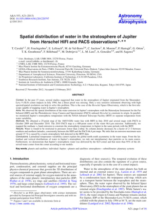
Line peak intensity [l/c-1] at 58.7 µm
-30-20-100102030
Arcsec
-30
-20
-10
0
10
20
30
Arcsec
-0.005
0
0.005
0.01
0.015
0.02
0.025
0.03
0.035
Line peak intensity [l/c-1] at 65.2 µm
-30-20-100102030
Arcsec
-30
-20
-10
0
10
20
30
Arcsec
0
0.002
0.004
0.006
0.008
0.01
0.012
0.014
0.016
-30-20-100102030
Arcsec
Line peak intensity [l/c-1] at 65.2 µm
Fig. 2. Water maps of the line peak intensity (=l/c-1, thus in % of the
continuum) at 58.7 and 65.2 μm observed by the PACS spectrometer on
December 8, 2009. Jupiter is represented by the black ellipse, and its
rotation axis is also displayed. The beam is represented by a gray filled
circle. Both maps indicate that there is less emission in the northern
hemisphere than in the southern (best seen in the limb emission).
and carried out complementary ground-based observations at the
NASA Infrared Telescope Facility (IRTF) in 2009 and 2010.
2.2. IRTF observations
2.2.1. IRTF/TEXES maps
On May 31 and October 17, 2009, we performed observations
with the Texas Echellon cross-dispersed Echelle Spectrograph
(TEXES; Lacy et al. 2002), mounted on the NASA IRTF
atop Mauna Kea. By achieving a spectral resolving power
of ∼80 000 in the ν4 band of methane (CH4) between 1244.8 and
1250.5 cm−1
(see Fig. 4), we were able to resolve the pressure-
broadened methane emission wing features, which give de-
tailed information on the vertical temperature profile from 0.01
Methane spectra from 0 and −13 latitude (red, black)
1245 1246 1247 1248 1249 1250
Wavenumber (cm−1
)
0.0
0.1
0.2
0.3
0.4
Radiance(ergs−1
cm−2
sr−1
/cm−1
)
0.0
0.2
0.4
0.6
0.8
1.0
TelluricTransmission
Fig. 4. Methane emission spectra from 13 ◦
S latitude (black) and from
the equator (red) showing the different spectral shape and strength from
the May 2009 observations with TEXES. The spectra are at an airmass
between 1 and 1.2. The blue curve represents the telluric transmission.
Owing to the high Jupiter/Earth velocity and the high spectral resolu-
tion achieved by TEXES, we were able to easily separate the Jovian
methane emission from the telluric methane absorption. Gaps in the
data are caused by telluric transmission regions that are too opaque to
retrieve useful data. The red and black spectra have been flat-fielded
by the black chopper wheel minus the sky emission, which performs a
first-order division of the atmosphere.
to 30 mbar. The data were reduced through the TEXES pipeline
reduction software package (Lacy et al. 2002), where they were
sky-subtracted, wavelength-calibrated, and flux-calibrated by
comparing them to observations of a black chopper wheel made
at the beginning of each set of four scan observations. We sub-
sequently processed the pipelined data through a purpose built
remapping software program to co-add all scan observations and
solve for the latitude1
and west longitude of each mapped step
and spaxel along the TEXES slit length. The data were then
zonally averaged and binned into latitude and airmass bin sizes
of 1−1.2, 1.2−1.5, 1.5−2.0, and 2.0−3.0 Jovian airmass. The lat-
itude bins (Nyquist-sampled spatial resolution) varied from 2 de-
grees at the sub-Earth point to 5 degrees at −60 degrees latitude.
2.2.2. IRTF/MIRSI maps
In addition to the TEXES observations, we recorded two sets
of radiometric images of Jupiter’s stratospheric thermal emis-
sion observed through a discrete filter with a FWHM of 0.8 μm,
centered at a wavelength of 7.8μm with the Mid-Infrared
Spectrometer and Imager (MIRSI; Kassis et al. 2008) that is
also mounted on the NASA IRTF. The radiance at this wave-
length is entirely controlled by thermal emission from the
ν4 vibrational-rotational fundamental of methane and emerges
from a broad pressure region in the middle of Jupiter’s strato-
sphere, 1−40 mbar (see Fig. 2 of Orton et al. 1991). Because
methane is well-mixed in Jupiter’s atmosphere, any changes
of emission are the result of changes in temperature around
this region of Jupiter’s stratosphere. The images were made (i)
on 25 June−1 July 2010, very close in time to the July 7 HIFI
observations, and (ii) on 5−6 December 2010, very close in time
to the December 15 PACS observations. An example of these
observations is shown in Fig. 5.
The data were reduced with the standard approach outlined
by Fletcher et al. (2009), in which they were sky-subtracted
with both short- (chop) and long-frequency (nod) reference im-
ages on the sky. The final results were co-additions of five in-
dividual images with the telescope pointing dithered around the
field of view to fill in bad pixels in the array and minimize the
effects of non-uniform sensitivities of pixels across the array.
Before coadding, the individual images were flat-fielded using a
1
All latitudes in this paper are planetocentric latitudes.
A21, page 4 of 16

5. T. Cavalié et al.: Spatial distribution of water in the stratosphere of Jupiter from Herschel HIFI and PACS observations
Fig. 5. IRTF/MIRSI radiance observations at 7.8 μm in the ν4 rotational-
vibrational band of methane in Jupiter. These radiance images, recorded
on June 30 (left) and December 5 (right), 2010, are essentially sensitive
to the stratospheric temperature between 1 and 40 mbar. The radiances
are given in erg/s/cm2
/cm−1
/ster.
reference to observations of a uniform heat source, a part of the
telescope dome. The images were also calibrated for absolute
radiance by convolving the filter function with spectra taken by
the Voyager IRIS and Cassini CIRS experiments, also described
in detail by Fletcher et al. (2009).
3. Modeling
3.1. Herschel data modeling
We analyzed the Herschel maps with a 1D radiative transfer
model that was improved from the model presented in Cavalié
et al. (2008a). Our code is written in ellipsoidal geometry
and accounts for the limb emission and the sub-observer point
position. We included the opacity caused by the H2-He-CH4
collision-induced absorption spectrum (Borysow et al. 1985,
1988; Borysow & Frommhold 1986) and by the far wings of
ammonia (NH3) and phosphine (PH3) lines. We used the JPL
Molecular Spectroscopy catalog (Pickett et al. 1998) as well
as H2/He pressure-broadening parameters parameters for water
lines from Dutta et al. (1993) and Brown & Plymate (1996).
As baseline, we used the same temperature profile as in
Cavalié et al. (2008b) and Cavalié et al. (2012), which was taken
from Fouchet et al. (2000) (see Fig. 6). The PACS observations
probe pressures lower than 2 mbar (see Fig. 7). In this way, we
constructed a series of thermal profiles, based on our nominal
profile, with 1-K-step temperature deviations at pressures lower
than 2 mbar to determine the necessary temperature deviations
from our nominal profile to fit the observations. These devia-
tions were then checked for consistency with our IRTF thermal
maps. The deviations from our nominal thermal profile are initi-
ated at 10 mbar to obtain a smooth transition toward the modified
thermal profile compared to our nominal profile (and to avoid in-
troducing a temperature inversion layer in the 1−10 mbar pres-
sure range for negative deviations). For each thermal profile, we
recomputed the pressure-altitude relationship assuming hydro-
static equilibrium. The resulting thermal profiles are shown in
Fig. 6.
Retrieving the water vertical profile from the HIFI spectra
will be the object of a forthcoming paper (Jarchow et al., in
prep.) and therefore will not be addressed here. We used pro-
files that are qualitatively representative of the IDP and SL9
sources. For the IDP source, we took the profile published in
Cavalié et al. (2008b), which corresponds to a water input flux
of 3.6 × 106
cm−2
s−1
. This profile was obtained with a photo-
chemical model that used the same thermal profile as our nomi-
nal profile and a standard K(z) profile (Moses et al. 2005). This
profile enables one to reproduce the average line intensity on the
HIFI map. For the SL9 source, we took an empirical profile in
0.0001
0.001
0.01
0.1
1
10
100
1000
10000
100 120 140 160 180 200
Pressure[mbar]
Temperature [K]
Fig. 6. Examples of temperature profiles used in this study. Our nominal
profile is displayed in red. The thermal profiles displayed in blue corre-
spond to cases in which the temperature at pressures lower than 2 mbar
is increased or decreased with 1-K steps from −14 to +15 K. The de-
viations from our nominal thermal profile are initiated at 10 mbar to
smooth the transition from the nominal profile at higher pressures to-
ward the modified thermal profile at lower pressures.
0.001
0.01
0.1
1
10
100
1000
10000
1e-18 1e-17 1e-16 1e-15 1e-14 1e-13
Pressure[mbar]
Contribution function [W.m -2
.Hz-1
.sr-1
.km-1
]
1670 GHz - nadir
1670 GHz - limb
66µm - nadir
66µm - limb
Fig. 7. Contribution functions of the water lines at 1669.9 GHz and
66.4 μm at their respective observed spectral resolutions for a pencil-
beam geometry. These profiles have been obtained with the water
profile used in this work (all water constrained to pressures lower
than 2 mbar).
which water is restricted to pressures lower than a given pres-
sure level p0 (to be determined by our analysis). Both profiles
are shown in Fig. 8.
The effect of the rapid rotation of the planet, which can
clearly be seen as red or blue Doppler shifts of the water lines on
the HIFI spectra (see Fig. 1) was taken into account, as well as
the spatial convolution due to the beams of the HIFI and PACS
instruments. Although the model assumes homogeneous temper-
ature and water abundance within a HIFI or PACS beam, the
geometry was fully treated. Indeed, the entire Jupiter disk was
divided into small elements, including the limb. We solved the
radiative transfer equation at each point and accounted for the
Doppler shifts caused by the rapid rotation of Jupiter before fi-
nally performing the spatial convolution by the instrument beam.
A21, page 5 of 16

6. A&A 553, A21 (2013)
0.001
0.01
0.1
1
10
100
1000
10000
1e-12 1e-11 1e-10 1e-09 1e-08 1e-07 1e-06
Pressure[mbar]
Mixing ratio
IDP
SL9
Fig. 8. Nominal water vertical profiles used in the analysis of the HIFI
and PACS maps. The IDP profile (red solid line) was computed with
the photochemical model of Cavalié et al. (2008b), using the nominal
thermal profile of Fig. 6 and a standard K(z) profile from Moses et al.
(2005). In the SL9 profile, a cut-off level was set to p0 = 2 mbar. This
is the highest value of p0 that enables reproducing all the HIFI lines. In
this profile, the water mixing ratio is 1.7 × 10−8
as in the central pixel
(number 13) of the HIFI map.
3.2. IRTF data modeling
Methane emission can be used to probe Jupiter’s stratospheric
temperatures because (i) the ν4 band of methane emits on the
Wien side of Jupiter’s blackbody curve; (ii) methane is well-
mixed throughout Jupiter’s atmosphere and only decreases off
at high altitudes because of diffusive separation (Moses et al.
2000); (iii) the deep volume mixing ratio is known from the
Galileo probe re-analysis results of Wong et al. (2004) to be
equal to 2.37±0.57 × 10−3
, resulting in a mole fraction of 2.05±
0.49 × 10−3
. For the TEXES data, we used the photochemical
model methane mole fraction profile from Moses et al. (2000)
with a deep value of 1.81 × 10−3
taken from the initial Galileo
probe results paper by Niemann et al. (1998) because it agrees
within errors with Wong et al. (2004). Moreover, the Moses et al.
(2000) model has been shown to agree with previous observa-
tions of Jupiter.
To infer Jupiter’s stratospheric temperatures from the
TEXES maps, we employed the automated line-by-line radiative
transfer model described in Greathouse et al. (2011). This model
uses the pressure-induced collisional opacity of H2-H2, H2-He,
and H2-CH4 as described by Borysow et al. (1985, 1988) and
Borysow & Frommhold (1986) and the molecular line opacity
for 12
CH4, 13
CH4, and CH3D from HITRAN (Rothman et al.
1998). It also varies the vertical temperature profile to repro-
duce the observed methane emission spectra. The resulting zon-
ally averaged temperature maps are displayed in Fig. 9. The
pressure range we are sensitive to with these observations is
0.01−30mbar.
A second approach to deriving stratospheric temperatures,
which we applied to our MIRSI maps, consists of using the ra-
diometrically calibrated versions of the 7.8 μm images. Although
these maps yield only temperatures at a single level (between 1
and 40 mbar), they can differentiate between the thermal models
shown in Fig. 6. Therefore, we simulated the 7.8 μm radiance we
would expect from the range of temperature profiles from Fig. 6
to create a table of radiance vs. emission angle. Then we de-
termined the upper-stratospheric temperature corresponding to
the profile that most closely produced the observed radiance at
each latitude/emission angle pair along the central meridian for
each date. Orton et al. (1991) used a similar approach in their
analysis of raster-scanned maps of Jupiter. The result is the tem-
perature maps that are shown in Fig. 10. The zonal variability
is much smaller than the meridional variability in each image,
validating the approach taken in examining the zonal-averaged
temperatures from the TEXES data shown in Fig. 9.
The Herschel observations are sensitive to pressures lower
than 2 mbar. This is why we created the range of thermal profiles
shown in Fig. 6, in which the profiles start to differ from one an-
other at pressures lower than 10 mbar. This introduces the main
limitation in our temperature derivation from the MIRSI images,
because these observations are sensitive to levels ranging from 1
to 40 mbar. To encompass the range of observed radiances that
are generated by higher temperatures in the 1−40 mbar range, we
therefore had to increase the range over which we were perturb-
ing the temperatures at pressures lower than 10 mbar. As a result,
the temperatures derived from the MIRSI images are excessively
high at latitudes corresponding to bright bands. Therefore, only
the trend in the latitudinal variation of the temperature can be
relied on rather than the values themselves.
4. Results
4.1. HIFI map
At 1669.9GHz and with the spectral resolution of HIFI, we
probed altitudes up to the 0.01 mbar pressure level, depending
on the observation geometry (see Fig. 7). The line opacity at
the central frequency at the observed spectral resolution but at
infinite spatial resolution is ∼10 at the nadir and ∼250 at the
limb. We first tested the IDP profile (presented in the previous
section) that fitted the SWAS and Odin observations in Cavalié
et al. (2008b, 2012). At Jupiter, this source should be steady and
spatially uniform (Selsis et al. 2004). In the case of a steady
local source, it would either show high concentrations at high
latitudes (for material transported in ionic form) or at low lat-
itudes (for material transported in neutral form). We detected
neither of these cases in the observations, although this diag-
nostic is limited by the relatively low spatial resolution. The re-
sult of the IDP model is displayed in Fig. 11. The IDP profile
fails to reproduce the observations in several aspects. Indeed, it
can be seen that this model produces lines that are too strong
in most of the northern hemisphere (pixels 6, 7, 15 and 16).
Figure 12 shows that if the water flux attributed to IDP is low-
ered to ∼2.0 × 106
cm−2
s−1
, the model matches the observa-
tions in terms of l/c but still overestimates the line width. The
main problem of this model is that the line wings are too broad
in most of the pixels. The only pixels in which the line wings
could be compatible with the data are pixels with the highest
noise. This means that the bulk of the stratospheric water is not
located just above the condensation level, i.e., at ∼20−30 mbar
as in the IDP model, but higher in altitude. The line shape of
the 556.9GHz water line as observed by SWAS and Odin al-
ready suggested that the IDP source was unlikely (Cavalié et al.
2008b). Consequently, the IDP model can be ruled out. In con-
trast, the SL9 profile gives much better results in the line wings
(see Fig. 11). We found that all line wings could be reproduced
A21, page 6 of 16

7. T. Cavalié et al.: Spatial distribution of water in the stratosphere of Jupiter from Herschel HIFI and PACS observations
Zonally averaged temperatures − May 2009
−80 −60 −40 −20 0 20 40 60 80
Planetocentric latitude (deg)
100
10
1
0.1
0.01
0.001
Pressure(mbar)
130 130
140 140
150 150
160
160
160
160
160
170
170
180
Zonally averaged temperatures − October 2009
−80 −60 −40 −20 0 20 40 60 80
Planetocentric latitude (deg)
100
10
1
0.1
0.01
0.001
Pressure(mbar)
130
140
150
160
160
160
170 170
170
170
180
−80 −60 −40 −20 0 20 40 60 80
Planetocentric latitude (deg)
130 130
140 140
150 150
160
160
160
160
160
170
170
18018080
Zonally averaged temperatures − October 2009
130
140
150
160
160
160
170 170
170
170
180
Fig. 9. Zonally averaged thermal maps as re-
trieved from IRTF/TEXES observations of the
ν4 band of methane carried out on May 31 and
October 17, 2009. The sensitivity ranges from
0.01 to 30 mbar.
provided that the p0 level was not set at pressures higher than
2 mbar2
. For the remainder of the paper, we have set the p0 level
to this value.
Before we more quantitatively analyze the SL9 model results
with regard to the HIFI observations, we focus on the PACS map
analysis using the information on the p0 level we derived above.
Because we already ruled out the IDP model at this stage, we do
not use it further in the analysis.
2
The value of p0 can be set to pressures lower than 2 mbar and still
reproduce the observations reasonably well, provided that additional
water was included in the model. Indeed, Doppler broadening is about
equal to pressure broadening around the 1 mbar level in Jupiter’s atmo-
sphere. Therefore, the line widths will be almost the same in models
with a value of p0 lower than 2 mbar.
4.2. PACS maps
We now use the PACS maps to separate the temperature and wa-
ter vapor variability. First, we can see that the line peak intensity
(=l/c − 1) maps (Figs. 2 and 3) present the same spatial struc-
ture. The highest emission is concentrated at the limb due to
limb-brightening in the line and limb-darkening in the contin-
uum. The main feature seen in these maps is the lack of emis-
sion around the northernmost region compared to the southern-
most region. However, we have to keep in mind that because the
observations are not spectrally resolved, all information on the
temperature and water column abundance is contained in the line
area. The line peak intensity alone only contains part of the in-
formation. Therefore, we fitted the line peak with an adjustable
line width in the model, which is the same as fitting the line area.
The line opacity at the central frequency at the observed spectral
A21, page 7 of 16

8. A&A 553, A21 (2013)
Fig. 10. IRTF/MIRSI radiance observations at 7.8 μm in the
ν4 rotational-vibrational band of methane, carried out on
25 June−1 July 2010 (top) and 5−6 December 2010 (bottom).
These observations are essentially sensitive to the stratospheric temper-
ature between 1 and 40 mbar. The color scale gives the correspondence
between radiances and stratospheric temperatures at 2 mbar, according
to our derivation procedure (see text for limitations). These maps
suggest that the northern hemisphere is generally warmer than the
southern hemisphere. The bright belt seen around 15 ◦
S in both maps
(as well as in the TEXES data; see Fig. 9) is a possible explanation for
the ∼4 K increase seen in the PACS 66.4 μm map between the equator
and 25 ◦
S. The bright dot seen in the 25 June−1 July 2010 map is Io
and had only marginal effects on the zonal mean results.
resolution but at infinite spatial resolution is ∼3 at the nadir and
∼100 at the limb.
To investigate whether this north-south asymmetry is caused
by the stratospheric temperature distribution or by the column
density spatial distribution, we analyzed the 66.4 μm emission
map considering two cases:
– We determined the spatial distribution of the tempera-
ture deviation from the nominal profile at pressures lower
than 2 mbar from our nominal thermal profile considering a
spatially uniform distribution of water. In this case, we set
the water mixing ratio to 2 × 10−8
for p ≤ 2 mbar, corre-
sponding to a column abundance of 3.7 × 1015
cm−2
. This
choice roughly corresponds to the average column found in
this map. Its choice is thus arbitrary to some extent but does
not affect the result, because we are interested in relative con-
trasts in temperature over Jupiter’s disk, not in absolute val-
ues of them.
– We determined the spatial distribution of the column density
considering a spatially uniform temperature profile (i.e., our
nominal profile).
4.2.1. Map of the stratospheric temperature deviation
from the nominal profile
We used the thermal profiles shown in Fig. 6 to check whether
latitudinal temperature variations could cause the line peak emis-
sion distribution observed in Fig. 3, assuming a spatially uniform
distribution of water. To do this, we fitted the line in each pixel
of the map by finding the most appropriate thermal profile and
retained the temperature deviation from the nominal profile as-
sociated to each pixel. The temperature deviation map associated
to the 66.4 μm observations is shown in Fig. 13. The uncertainty
on the line peak values is in the range of 3−10%, which trans-
lates into an uncertainty of 1−3 K on the derived temperature
deviation. Another way to evaluate the uncertainty on the tem-
perature is to see the variations of the temperature around a given
latitude. Although the atmosphere radiative timescale is 3 orders
of magnitude longer than the rotation period (Flasar 1989), vari-
ations of several K in the zonal temperatures at 1 mbar, probably
caused by a Rossby wave trapped at certain latitudes, have been
reported by Flasar et al. (2004). However, at our spatial resolu-
tion, the temperature should be smoothed in longitude compared
to Flasar et al.’s observations. After checking the temperatures
in several narrow latitudinal bands, we found a scatter of ∼3 K
on the temperature, which agrees with the uncertainty range we
derived.
The 66.4 μm map in Fig. 13 shows two interesting structures
that can also be better seen in a representation of the temperature
deviation from the nominal profile as a function of latitude. Such
a latitudinal section is shown in Fig. 14.
First, a north-south contrast of 10−15 K (with higher tem-
peratures in the southern hemisphere) is required to reproduce
the global north-south asymmetry seen in the line peak emission.
This picture contradicts the TEXES maps from 2009 (see Fig. 9).
In these maps, we see large meridional variations at 2 mbar (see
Fig. 14), of the same order of magnitude as in our PACS map
(∼10 K). These variations correlate quite well with those seen
by Fletcher et al. (2011) at 5 mbar in 2009−2010. But there
is no evidence for a global meridional asymmetry. Moreover,
there clearly are changes in the stratospheric temperature field
between 2009 and 2010, as shown by the thermal maps we re-
trieved from the 7.8 μm IRTF/MIRSI images we captured a few
days before the HIFI and PACS maps were produced (see in
Fig. 10). However, these changes do not work in favor of the
temperature variability hypothesis to explain the water emission
maps. On the contrary, the Jovian quasiquadriennial oscillation
(Leovy et al. 1991) creates a bright band north of the equator that
we only marginally see in Fig. 13. Accordingly, the MIRSI ob-
servations even suggest that there the temperatures are higher in
the northern hemisphere than in the southern hemisphere in the
pressure range we are sensitive to. The opposite would have been
necessary to explain the water emission maps. Consequently, the
asymmetry we see in the water emission maps has to be due to
an hemispherical asymmetry in the water distribution.
The second structure we see in the 66.4 μm map is a temper-
ature increase of ∼4 K between 25 ◦
S and the equator. There is
a good correlation between this feature and a warm temperature
belt seen consistently between 1 and 30 mbar in the MIRSI and
TEXES data and in Fletcher et al. (2011) around 15 ◦
S. This fea-
ture likely results from the spatial convolving of this warm belt
(see Fig. 14). We discuss it in Sect. 5.1.
Now that we have proven that a global latitudinal temper-
ature variation is not the cause for the north-south asymmetry
seen in the line peak intensity maps, we can derive the column
density map that reproduces the observations.
4.2.2. Column density map
Here, we assumed that our nominal temperature profile is valid
at any latitude/longitude and locally rescaled the water vertical
profile, i.e., the water column density, to fit the line in each pixel.
The computed column densities are representative of averages
A21, page 8 of 16

9. T. Cavalié et al.: Spatial distribution of water in the stratosphere of Jupiter from Herschel HIFI and PACS observations
-30
-20
-10
0
10
20
30
-30-20-100102030
Offset[arcsec]
Offset [arcsec]
data
SL9
IDP
0.9
1
1.1
1.2
1.3
1.4
1.5
-60-40-20 0 20 40 60
1
0.9
1
1.1
1.2
1.3
1.4
1.5
-60-40-20 0 20 40 60
2
0.9
1
1.1
1.2
1.3
1.4
1.5
-60-40-20 0 20 40 60
3
0.9
1
1.1
1.2
1.3
1.4
1.5
-60-40-20 0 20 40 60
4
0.9
1
1.1
1.2
1.3
1.4
1.5
-60-40-20 0 20 40 60
5
0.9
1
1.1
1.2
1.3
1.4
1.5
-60-40-20 0 20 40 60
6
0.9
1
1.1
1.2
1.3
1.4
1.5
-60-40-20 0 20 40 60
7
0.9
1
1.1
1.2
1.3
1.4
1.5
-60-40-20 0 20 40 60
8
0.9
1
1.1
1.2
1.3
1.4
1.5
-60-40-20 0 20 40 60
9
0.9
1
1.1
1.2
1.3
1.4
1.5
-60-40-20 0 20 40 60
10
0.9
1
1.1
1.2
1.3
1.4
1.5
-60-40-20 0 20 40 60
11
0.9
1
1.1
1.2
1.3
1.4
1.5
-60-40-20 0 20 40 60
12
0.9
1
1.1
1.2
1.3
1.4
1.5
-60-40-20 0 20 40 60
13
0.9
1
1.1
1.2
1.3
1.4
1.5
-60-40-20 0 20 40 60
14
0.9
1
1.1
1.2
1.3
1.4
1.5
-60-40-20 0 20 40 60
15
0.9
1
1.1
1.2
1.3
1.4
1.5
-60-40-20 0 20 40 60
16
0.9
1
1.1
1.2
1.3
1.4
1.5
-60-40-20 0 20 40 60
17
0.9
1
1.1
1.2
1.3
1.4
1.5
-60-40-20 0 20 40 60
18
0.9
1
1.1
1.2
1.3
1.4
1.5
-60-40-20 0 20 40 60
19
0.9
1
1.1
1.2
1.3
1.4
1.5
-60-40-20 0 20 40 60
20
0.9
1
1.1
1.2
1.3
1.4
1.5
-60-40-20 0 20 40 60
Line-to-continuumratio
Velocity [km.s-1
]
21
0.9
1
1.1
1.2
1.3
1.4
1.5
-60-40-20 0 20 40 60
22
0.9
1
1.1
1.2
1.3
1.4
1.5
-60-40-20 0 20 40 60
23
0.9
1
1.1
1.2
1.3
1.4
1.5
-60-40-20 0 20 40 60
24
0.9
1
1.1
1.2
1.3
1.4
1.5
-60-40-20 0 20 40 60
25
Fig. 11. Water 5 × 5 raster map at 1669.9 GHz obtained with Herschel/HIFI on July 7, 2010, expressed in terms of l/c and smoothed to a spectral
resolution of 12 MHz (observation are plotted in black). Jupiter is represented with the red ellipse, and its rotation axis is also displayed. The black
crosses indicate the center of the various pixels after averaging the H and V polarizations. The beam is represented for the central pixel by the red
dotted circle.These high S/N observations rule out the IDP source model (red lines) because they result (i) in narrower lines than the ones produced
by the IDP model; and (ii) in a non-uniform spatial distribution of water. Even if the flux in the northernmost pixels is adjusted to lower values to
fit the l/c, the IDP model fails to reproduce the line wings (see Fig. 12). By adjusting the local water column density by rescaling the SL9 vertical
profile, we find that an SL9 model (blue line), in which all water resides at pressures lower than 2 mbar, enables one to reproduce the observed
map.
over the PACS beam. The resulting maps are displayed in Fig. 15
and a latitudinal section taken from the 66.4 μm map is shown in
Fig. 16. The uncertainty on the line peak values translates into
an uncertainty of up to 20% on the column density values. This
is consistent with the scatter we find in narrow latitudinal bands
(∼15%). If we had used a physical profile for the SL9-material
evolution instead of an empirical one for water, we could have
ended up with column density values different by a factor of up
to 2 (with the same level of uncertainties). One needs to know
the true vertical profile to retrieve the true values of the local
water column.
The 66.4 μm map and the corresponding latitudinal section
show a general trend in the latitudinal distribution of the derived
column densities. Indeed, we see an increase by a factor of 2−3
from the northernmost latitudes to the southern latitudes. This
kind of distribution was anticipated by Lellouch et al. (2002),
though with a much lower contrast, from their SL9 model. They
expected a contrast of only 10% between 60 ◦
S and 60 ◦
N at
infinite spatial resolution in 2007. Here, we observe a factor
of 2−3 contrast between 60◦
S and 60 ◦
N after spatial convolu-
tion by the instrument beam. This should translate into an even
stronger contrast at infinite spatial resolution.
A21, page 9 of 16

10. A&A 553, A21 (2013)
0.9
1
1.1
1.2
1.3
1.4
1.5
-60 -40 -20 0 20 40 60
velocity [km.s
-1
]
6
0.9
1
1.1
1.2
1.3
1.4
1.5
-60 -40 -20 0 20 40 60
velocity [km.s
-1
]
15
0.9
1
1.1
1.2
1.3
1.4
1.5
-60 -40 -20 0 20 40 60
Line-to-continuumratio
velocity [km.s
-1
]
16
Fig. 12. Zoom on the northernmost pixels 6, 15 and 16 of the HIFI map. The SL9 model is displayed in blue, while the IDP model with a flux
of 3.6 × 106
cm−2
s−1
is plotted in red. The IDP model overestimates both the l/c and the line width in each pixel. Even if the IDP flux is lowered
to 2.0 × 106
cm−2
s−1
(green line) to roughly fit the l/c, it still fails to fit the wings. A model based on the philosophy of the “hybrid” model of
Lellouch et al. (2002) with the SL9 source and a background IDP source with a flux of 8 × 104
cm−2
s−1
, corresponding to the upper limit placed
on the IDP source by the authors, is shown in orange. This model can barely be distinguished from the pure SL9 model, which means that an IDP
background source is compatible with our observations.
Temperature deviation [K] - H2O at 66.4 µm
-30-20-100102030
Arcsec
-30
-20
-10
0
10
20
30
Arcsec
-20
-15
-10
-5
0
5
10
15
Fig. 13. Map of the temperature deviation (in
K) from the nominal thermal profile assum-
ing a spatially uniform distribution of water,
as derived from the 66.4 μm map. Jupiter is
represented by the black ellipse, and its rota-
tion axis is also displayed. The beam is repre-
sented by the gray filled circle. A relative dif-
ference of 10−15 K in the high stratospheric
temperatures between the northern and south-
ern latitudes is required to reproduce the ob-
servations. A warm south equatorial region
(0−25 ◦
S) of ∼4 K higher stratospheric tem-
peratures is identified in this map (see also
Fig. 14).
We applied the same methodology as for the PACS map to
derive the local column density from the HIFI map, still as-
suming a spatially uniform temperature. The resulting map is
shown in Fig. 17. The uncertainty on the column abundance
derivation is on the order of 20% in the HIFI pixels despite the
high S/N, because the line is optically thick. We find that the
column abundance increases from the northernmost latitude to
the southern latitudes by a factor of ∼3. The general trend as
a function of latitude as well as the highest values of the wa-
ter column (4−5 × 1015
cm−2
) fully agree with the PACS results
obtained at 66.4 μm and therefore confirm our results.
5. Discussion
5.1. A local temperature maximum or an additional source
of water around 15 ◦
S?
In the 66.4 μm map analysis (Sect. 4.2.1), we found that the
emission between the equator and 25 ◦
S could be explained by
either an about 4 K warmer stratospheric temperature and/or a
higher water column density (or even a combination of both),
over the PACS beam.
A21, page 10 of 16

11. T. Cavalié et al.: Spatial distribution of water in the stratosphere of Jupiter from Herschel HIFI and PACS observations
-15
-10
-5
0
5
10
-80 -60 -40 -20 0 20 40 60 80
145
150
155
160
165
170
175
Temperaturedeviation[K]
Temperature[K]
Planetocentric latitude
TEXES - 05/2009
TEXES - 10/2009
MIRSI - 07/2010
MIRSI - 12/2010
PACS - 12/2010
Fig. 14. Latitudinal section of the temperature deviation from the nom-
inal profile as derived from the 66.4 μm map (black points), assuming a
spatially uniform distribution of water. Only the pixels within the plane-
tary disk are represented here. The temperatures at a pressure of 2 mbar
as retrieved from our IRTF/TEXES observations are also displayed (red
line for the May 2009 data and blue line for the October 2009 data)
as well as the temperatures derived from our IRTF/MIRSI data (green
for July 2010 and yellow for December 2010). The temperatures de-
rived from the MIRSI images are averages for the pressure range the
observations are sensitive to (1−40 mbar). We applied to these values
an offset of −20 K to bring them to the same scale as the TEXES values
(see Sect. 3.2 for the reasons why we obtained these high values from
the MIRSI data). The warm temperature belt seen around 15 ◦
S is the
most probable cause for the enhanced emission seen at these latitudes in
our 66.4 μm map (see Fig. 13). There is only marginal evidence in the
water emission observations for the warm belt seen in the IRTF/MIRSI
data around 30 ◦
N.
The IRTF/MIRSI images unveil a warm belt around 15 ◦
S at
pressures between 1 and 40 mbar (see Fig. 5), also seen in the
data of Fletcher et al. (2011) at 5 mbar. The temperature maps
retrieved from the IRTF/TEXES data locate such a belt at this
latitude in the 1−10 mbar pressure range (see Fig. 9) and it is
most obvious at 2 mbar (see Fig. 14). Given that the tempera-
ture excess needed over the PACS beam to fit the data is ∼4 K,
this warm belt is probably sufficient to explain the enhanced wa-
ter emission in this latitudinal range. This warm belt also im-
plies that the water condensation level is located at a slightly
lower altitude, allowing higher column densities of water at these
latitudes.
On the other hand, if the warm belt is not sufficient and if the
water column is indeed higher at these latitudes (independently
of any temperature effect), this means that this extra water is pro-
vided by an additional source. What kind of source could that
be? A local source (rings/satellites) that would generate these
spatial properties seems unlikely. If the material were trans-
ported from the source to Jupiter in neutral form, the deposi-
tion latitude should be centered on the equator. According to
Hartogh et al. (2011), this is how the Enceladus torus feeds
Saturn’s stratosphere in water. A second possibility is the de-
position of ionized material (with a high charge-to-mass ratio)
at latitudes that are magnetically connected to the source(s), as
proposed by Connerney (1986). According to his work, a source
depositing material at ∼10 ◦
S would probably need to be located
at 1.1 planetary radii, in the case of Saturn. Because Jupiter’s
magnetic field is 20 times stronger than Saturn’s, this would im-
ply that a hypothetical source depositing material around 15 ◦
S
would need to be even closer to the planet than 1.1 Jupiter radii,
a zone where there is no such source. There is no reason why a
source like the IDP would deposit material only around 15 ◦
S.
In addition to that, an increase by a factor of ∼2 of the water
column due to a local source or an IDP source should result
in broader line widths in the pixels centered on the equator in
the HIFI map, an effect evidently absent from Fig. 11. Finally,
another possible source is an additional comet impact. The only
known events are two impacts that have been detected in Jupiter
between the SL9 event and our 2010 PACS observation. The
first one occurred on July 19, 2009, but at a planetocentric lat-
itude of 55 ◦
S (Sánchez-Lavega et al. 2010; Orton et al. 2011).
Interestingly, the second observed impact occurred on June 3,
2010, at a planetocentric latitude of 14.◦
5 S (Hueso et al. 2010).
According to Hueso et al. (2010), this impactor had a size of
8−13 m. According to Fig. 16, the excess of H2O column in
this latitude region is on the order of ∼1015
cm−2
. The latitu-
dinal band extending from 25 ◦
S to the equator has a surface
area of 1.35 × 1020
cm2
. The excess of water then corresponds
to 4 × 109
kg of water, i.e., ∼3500 times the mass of a 3 m im-
pactor consisting of pure water. It is thus unlikely that this extra
water (if any) located between 25 ◦
S and the equator is due to an
additional external source.
Finally, we recall that the highest emission seen between
25 ◦
S and the equator can most probably be attributed to the tem-
perature increase in this region as seen in the MIRSI and TEXES
maps (Figs. 9, 10 and 14).
5.2. Spatial distribution of water in Jupiter
The HIFI and PACS maps contain horizontal information on
the water distribution in Jupiter’s stratosphere. Because HIFI re-
solves the line shapes of the water emission at 1669.9GHz, the
HIFI map also contains information on the vertical distribution
of the species if they are located at pressures lower than 1 mbar.
As stated previously, the precise shape of the vertical water
profile will be retrieved from the 556.9, 1097.4 and 1669.9 GHz
water lines observed at very high S/N with HIFI in the frame-
work of the HssO Key Program and shall therefore be discussed
in detail in a future dedicated paper (Jarchow et al., in prep.).
However, we tested profiles that are qualitatively compatible
with the IDP and SL9 sources. The spectral line shapes ob-
served with the HIFI very high resolution confirm that the bulk
of water resides at lower pressure levels (i.e., at pressures lower
than 2 mbar) than would be the case with a steady IDP source.
This result agree well with the prediction of Moreno et al. (2003)
for the p0 level (1 mbar) for CO, hydrogen cyanide (HCN), and
carbon monosulfide (CS) 20 years after the SL9 impacts. Cavalié
et al. (2012) studied the temporal evolution of the disk-averaged
water line at 556.9 GHz with the Odin space telescope for almost
a decade. They developed two models that could fit the tenta-
tively seen decrease in the line contrast. In a first model, they ten-
tatively increased the vertical eddy diffusion K(z) by a factor of 3
at 1 mbar to remove more water by condensation. The line pro-
files in the HIFI map now show that this hypothesis is not valid
and that the bulk of water remains at higher levels (p0 ≤ 2 mbar)
than in their model, where the bulk of water had spread quite
uniformly as a function of pressure down to the condensation
level (see their Fig. 10). This means that the decrease of the line-
to-continuum ratio at 556.9 GHz that they have tentatively ob-
served has to be explained by the removal of water at the mbar
and submbar levels and not by condensation. In a second model,
Cavalié et al. (2012) approximately incorporated dilution effects
from horizontal diffusion and chemical losses due to conversion
of OH radicals (photolytical product of H2O) into CO2 based
on the predictions of Lellouch et al. (2002) for their previously
published temporal evolution model (Cavalié et al. 2008b). The
water vertical profile used in Cavalié et al. (2008b) was based on
the philosophy of the “hybrid model” of Lellouch et al. (2002),
which took into account a low IDP flux of 4 × 104
cm−2
s−1
. This
second model of Cavalié et al. (2012) has several advantages in
A21, page 11 of 16

12. A&A 553, A21 (2013)
Column density [cm-2
] - H2O at 66.4 µm
-30-20-100102030
Arcsec
-30
-20
-10
0
10
20
30
Arcsec
0
1e+15
2e+15
3e+15
4e+15
5e+15
6e+15
7e+15
8e+15
9e+15
Fig. 15. Column density of water (in cm−2
), as
derived from the 66.4 μm map. Jupiter is rep-
resented by the black ellipse, and its rotation
axis is also displayed. The beam is represented
by the gray filled circle. In the south equatorial
region (0−25 ◦
S), the emission maximum iden-
tified in this map is most probably caused by a
temperature effect and not by a local maximum
of the column density.
that enough water is lost as a function of time to reproduce the
temporal evolution of the 556.9GHz line, and it keeps a stan-
dard K(z) profile and thus keeps the bulk of water at pressures
compatible with our HIFI results. In this sense, it reconciles the
Odin and our HIFI submillimeter observations of water with
the infrared observations of ISO. Another advantage is that this
model also accounts for a background IDP source with a flux
of 4 × 104
cm−2
s−1
. According to our computations, adding an
IDP source of that magnitude is not inconsistent with our obser-
vations, because such a low flux only marginally affects the line
shape at 1669.9 GHz and 66.4 μm (e.g., Fig. 12). Even a model
accounting for a background source due to IDP with a flux cor-
responding to the upper limit derived by Lellouch et al. (2002)
(8 × 104
cm−2
s−1
) remains compatible with our data3
(see
Fig. 12). We are thus able to quantify how much of the observed
water can be attributed to the SL9 impact. The disk-averaged
column density of this SL9 + background IDP model (with a
flux of 8 × 104
cm−2
s−1
) is ∼3 × 1015
cm−2
, while the column
density of the background IDP source alone is ∼1014
cm−2
. This
means that more than 95% of the observed water comes from
SL9 according to our models. These results are somewhat differ-
ent from those obtained by Lellouch et al. (2002). These authors
found a disk-averaged column of 1.5 × 1015
cm−2
from their
SL9 + background IDP model and 4.5 × 1014
cm−2
for their
background IDP model with a flux of 8 × 104
cm−2
s−1
, imply-
ing that up to 30% of the water could be due to IDP. These dif-
ferences may arise from a different choice of chemical scheme,
temperature, and vertical eddy mixing profiles. But both results
3
This possible additional background source could also be attributed
to a flow of smaller comets that would have impacted Jupiter at random
latitudes in the last tens to a couple of hundreds of years, for which
the vertical distribution of water would resemble that of a background
IDP source.
essentially show that SL9 is by far the main source of water in
Jupiter’s stratosphere.
The HIFI and the 66.4 μm PACS maps consistently show
a north-south asymmetry that cannot be attributed to a hemi-
spheric asymmetry in the stratospheric temperatures but to an
asymmetry in the water column abundance. If we omit the
25 ◦
S-to-equator band from the meridional distribution observed
by PACS shown in Fig. 16, which is most probably a result of a
local temperature increase, we see that the water column looks
roughly constant in the southern hemisphere and decreases lin-
early by a factor of 2−3 poleward in the northern hemisphere.
This behavior is not expected from a IDP source but is consis-
tent with the SL9 source, because the comet has hit the planet
at 44 ◦
S. Although the observations have taken place more than
15 years after the SL9 impacts, a remnant of the latitudinal asym-
metry that was predicted by Lellouch et al. (2002) is now demon-
strated, thus validating the SL9 source.
We have to keep in mind that, unlike Lellouch et al. (2006)
for HCN and CO2, we do not have access to latitudes higher
than ∼60◦
because of the observation geometry and beam con-
volution. It would thus be hazardous to directly compare of the
water distribution with the distributions of HCN and CO2 previ-
ously observed by Lellouch et al. (2006). They also correspond
to different post-impact observation dates.
Lellouch et al. (2002) used a horizontal model that accounted
for meridional eddy diffusion and a simplified chemical scheme
for oxygen species to model the temporal evolution of the water
column as a function of latitude. They derived a horizontal eddy
diffusion coefficient of Kh = 2 × 1011
cm2
s−1
, constant in lati-
tude, and a H2O/CO ratio of 0.11 from their observed CO2 hor-
izontal distribution and disk-averaged water column. According
to the results of this model, the contrast predicted for 2007 (i.e.,
even earlier than our Herschel maps) was ∼10% at infinite spa-
tial resolution. The contrast measured with PACS at 66.4 μm is
A21, page 12 of 16

13. T. Cavalié et al.: Spatial distribution of water in the stratosphere of Jupiter from Herschel HIFI and PACS observations
0
1e+15
2e+15
3e+15
4e+15
5e+15
6e+15
7e+15
-80 -60 -40 -20 0 20 40 60 80
H2Ocolumnabundance[cm-2
]
Planetocentric latitude
Fig. 16. Latitudinal section of the beam-convolved column density of
water as derived from the 66.4 μm map. Only the pixels within the plan-
etary disk are represented here. The peak values around 15 ◦
S can most
probably be attributed to the warmer temperatures observed around this
latitude. The marginal increase seen around 30 ◦
N could be due to the
bright band detected at these latitudes in 2010 in the IRTF/MIRSI ob-
servations (see Fig. 14).
Column density [cm -2
] -H2O at 1669.9 GHz
-30-20-100102030
Arcsec
-30
-20
-10
0
10
20
30
Arcsec
1e+15
1.5e+15
2e+15
2.5e+15
3e+15
3.5e+15
4e+15
4.5e+15
5e+15
Fig. 17. Beam-convolved column density of water (cm−2
) map as de-
rived from the HIFI observations at 1669.9 GHz. The beam is repre-
sented for the central pixel by the red circle.
already higher despite the beam convolution, which results in
its attenuation. The deconvolution of the observed contrast to
constrain horizontal transport is beyond the scope of this pa-
per. However, we anticipate that if it were only due to eddy dif-
fusion, the meridional distribution of water in Jupiter’s strato-
sphere would require lower values for Kh. Lellouch et al. (2006)
showed that the HCN meridional distribution in December 2000
(6.5 years after the impacts) could not be reproduced by us-
ing the latitudinally constant meridional eddy diffusion coeffi-
cient Kyy of Griffith et al. (2004). They rather had to invoke not
only a Kyy variable in latitude (θ) with peak values of Kyy ∼
2.5 × 1011
cm2
s−1
, consistent with low spatial resolution mea-
surements of Moreno et al. (2003), and a significant decrease of
Kyy by an order of magnitude poleward of 40◦
, but also equator-
ward advective transport with wind velocities of ∼7 cm s−1
. The
equatorward advective wind results in a slower contamination of
the northern hemisphere. According to this work and to Moreno
et al. (2003), water and HCN are located at the same pressure
level. If confirmed, they should be subject to the same hori-
zontal transport regime. The philosophy of the transport model
of Lellouch et al. (2006) seems to agree with our observations,
but more modeling work is needed to check the consistency of
their Kyy(θ) and wind velocity profiles.
We recall that the water column density values derived in
this paper correspond to values convolved by the PACS beam.
Because the 66.4 μm water line targeted for the mapping with
PACS, from which the column densities were derived, is opti-
cally thick, there is no linear relation between the column den-
sities and the observed lines. Therefore, it is not possible to
simply spatially convolve the results of a diffusion model to
compare it with our observation results. The confirmation of
the validity of the horizontal model from Lellouch et al. (2006)
with those data thus requires reproducing the observed map
with a 2D (for geometry) radiative transfer model that could be
fed with the water latitude-dependent distribution output of the
diffusion+advection model. The problem is even more compli-
cated because of the sensitivity of water to photolysis in Jupiter’s
high stratosphere and to condensation in the low stratosphere.
Accordingly, unlike HCN and CO2, water is not chemically sta-
ble and cannot be considered as an ideal tracer for horizontal dy-
namics. A 2D/3D photochemical model including oxygen chem-
istry is therefore necessary to derive constraints on Kyy(θ) and
on advection in Jupiter’s stratosphere at the mbar level. Such
a model would also enable one to retrieve a reliable mass of
the water that was initially deposited by the comet from these
Herschel observations. Recent work by Dobrijevic et al. (2010,
2011) now enables reducing the size of chemical schemes to ac-
ceptable sizes to extend existing 1D photochemical models to
2D/3D by identifying key reactions in the more complete chem-
ical schemes of 1D models. These reduced chemical schemes
will facilitate the emergence of 2D/3D photochemical models
because they reduce the computational time for chemistry by one
to two orders of magnitude.
6. Conclusion
We have performed the first spatially resolved observations of
water in the stratosphere of Jupiter with the HIFI and PACS in-
struments of the Herschel Space Observatory in 2009−2010 to
determine its origin. In parallel, we monitored the stratospheric
temperature in Jupiter with the NASA IRTF in the same periods
to separate temperature from water variability in the Herschel
maps.
We found that the shape of the water lines at 1669.9 GHz in
the HIFI map recorded at very high spectral resolution proves
that the bulk of water resides at pressures lower than 2 mbar.
This rules out any steady source, like the IDP source, in
which water would be present down to the condensation level
(∼20−30mbar). A uniform source is also ruled out by both the
HIFI and PACS maps. Indeed, the observations show a north-
south asymmetry in the emission. The water column is roughly
constant in the southern hemisphere and decreases linearly by
a factor of 2−3 poleward in the northern hemisphere, at the
spatial resolution of the observations. This distribution cannot
be attributed to a hemispheric asymmetry in the stratospheric
temperatures, according to our IRTF observations, but rather to
meridional variability of the water column abundance. Thus, the
spatial distribution of water in Jupiter’s stratosphere is clear ev-
idence that a recent comet, i.e., the Shoemaker-Levy 9 comet,
is the principal source of water in Jupiter. What we observe to-
day is a remnant of the oxygen delivery by the comet at 44 ◦
S in
July 1994.
A21, page 13 of 16

14. A&A 553, A21 (2013)
It is possible that other sources like IDP or icy satellites
may coexist at Jupiter, but, as demonstrated by this work, with
other spatial distribution properties and lower magnitudes than
the SL9 source. The upper limit derived for an IDP source by
Lellouch et al. (2002) (with a flux of 8 × 104
cm−2
s−1
) is consis-
tent with the Herschel observations, meaning that at least 95%
of the observed water comes from the SL9 comet and subse-
quent (photo)-chemistry in Jupiter’s stratosphere according to
our models, as of today.
Although they reached their objective of determining the ori-
gin of the bulk of stratospheric water in Jupiter, the mapping
observations we presented have insufficient latitudinal resolu-
tion and a lack of information at latitudes higher than ∼60◦
to
assess the relative magnitude of all possible water sources at
Jupiter. The Submillimetre Wave Instrument (Hartogh et al.
2009a) is an instrument proposed for the payload of the recently
selected Jupiter Icy Moon Explorer (JUICE), an L-class mission
of the ESA Cosmic Vision 2015−2025 program, which is to be
launched in 2022 and will study the Jovian system for 3.5 years
starting in 2030. This instrument has several key objectives, one
of which is to map in 3D SL9-derived species in the stratosphere
of Jupiter with scale height vertical resolution and 1◦
resolution
in latitude. It also proposes to measure the isotopic ratios in wa-
ter and CO. The combination of these measurements will enable
us to separate the spatial and isotopic signatures of all possible
sources and their relative magnitude at Jupiter.
Acknowledgements. T. Cavalié wishes to thank J. Brillet for providing him
with his baseline ripple removal tool for the purposes of this work. T. Cavalié
acknowledges funding from the Centre National d’Études Spatiales (CNES).
M. de Val-Borro acknowledges support from the Special Priority Program 1488
of the German Science Foundation, and grants NSF AST-1108686 and NASA
NNX12AH91H. G. Orton acknowledges funding from the National Aeronautics
and Space Administration to the Jet Propulsion Laboratory, California Institute
of Technology. T. Greathouse acknowledges funding from NASA PAST grant
NNX08AW33G and was supported as a Visiting Astronomer at the Infrared
Telescope Facility, which is operated by the University of Hawaii under
Cooperative Agreement no. NNX-08AE38A with the National Aeronautics
and Space Administration, Science Mission Directorate, Planetary Astronomy
Program. F. Billebaud wishes to thank the Programme National de Planétologie
(PNP) of the Institut National des Sciences de l’Univers (INSU) for pluri-
annual funding on this project. HIFI has been designed and built by a con-
sortium of institutes and university departments from across Europe, Canada
and the United States under the leadership of SRON Netherlands Institute
for Space Research, Groningen, The Netherlands and with major contribu-
tions from Germany, France and the US. Consortium members are: Canada:
CSA, U.Waterloo; France: CESR, LAB, LERMA, IRAM; Germany: KOSMA,
MPIfR, MPS; Ireland, NUI Maynooth; Italy: ASI, IFSI-INAF, Osservatorio
Astrofisico di Arcetri-INAF; Netherlands: SRON, TUD; Poland: CAMK, CBK;
Spain: Observatorio Astronómico Nacional (IGN), Centro de Astrobiología
(CSIC-INTA). Sweden: Chalmers University of Technology − MC2, RSS &
GARD; Onsala Space Observatory; Swedish National Space Board, Stockholm
University − Stockholm Observatory; Switzerland: ETH Zurich, FHNW; USA:
Caltech, JPL, NHSC. PACS has been developed by a consortium of insti-
tutes led by MPE (Germany) and including UVIE (Austria); KUL, CSL,
IMEC (Belgium); CEA, OAMP (France); MPIA (Germany); IFSI, OAP/AOT,
OAA/CAISMI, LENS, SISSA (Italy); IAC (Spain). This development has been
supported by the funding agencies BMVIT (Austria), ESA-PRODEX (Belgium),
CEA/CNES (France), DLR (Germany), ASI (Italy), and CICT/MCT (Spain).
Data presented in this paper were analyzed using HIPE is a joint development
by the Herschel Science Ground Segment Consortium, consisting of ESA, the
NASA Herschel Science Center, and the HIFI, PACS and SPIRE consortia. This
development has been supported by national funding agencies: CEA, CNES,
CNRS (France); ASI (Italy); DLR (Germany). Additional funding support for
some instrument activities has been provided by ESA. We are grateful to an
anonymous referee for the constructive comments about this manuscript.
References
Bézard, B., Lellouch, E., Strobel, D., Maillard, J.-P., & Drossart, P. 2002, Icarus,
159, 95
Bjoraker, G. L., Stolovy, S. R., Herter, T. L., Gull, G. E., & Pirger, B. E. 1996,
Icarus, 121, 411
Borysow, A., & Frommhold, L. 1986, ApJ, 304, 849
Borysow, J., Trafton, L., Frommhold, L., & Birnbaum, G. 1985, ApJ, 296, 644
Borysow, J., Frommhold, L., & Birnbaum, G. 1988, ApJ, 326, 509
Brown, L. R., & Plymate, C. 1996, J. Quant. Spec. Radiat. Transf., 56, 263
Cavalié, T., Billebaud, F., Biver, N., et al. 2008a, Planet. Space Sci., 56, 1573
Cavalié, T., Billebaud, F., Fouchet, T., et al. 2008b, A&A, 484, 555
Cavalié, T., Billebaud, F., Dobrijevic, M., et al. 2009, Icarus, 203, 531
Cavalié, T., Hartogh, P., Billebaud, F., et al. 2010, A&A, 510, A88
Cavalié, T., Biver, N., Hartogh, P., et al. 2012, Planet. Space Sci., 61, 3
Connerney, J. E. P. 1986, Geophys. Res. Lett., 13, 773
de Graauw, T., Helmich, F. P., Phillips, T. G., et al. 2010, A&A, 518, L6
Dobrijevic, M., Cavalié, T., Hébrard, E., et al. 2010, Planet. Space Sci., 58, 1555
Dobrijevic, M., Cavalié, T., & Billebaud, F. 2011, Icarus, 214, 275
Dutta, J. M., Jones, C. R., Goyette, T. M., & De Lucia, F. C. 1993, Icarus, 102,
232
Feuchtgruber, H., Lellouch, E., de Graauw, T., et al. 1997, Nature, 389, 159
Flasar, F. M. 1989, NASA Spec. Publ., 494, 324
Flasar, F. M., Kunde, V. G., Achterberg, R. K., et al. 2004, Nature, 427, 132
Fletcher, L. N., Orton, G. S., Yanamandra-Fisher, P., et al. 2009, Icarus, 200, 154
Fletcher, L. N., Orton, G. S., Rogers, J. H., et al. 2011, Icarus, 213, 564
Fouchet, T., Lellouch, E., Bézard, B., et al. 2000, A&A, 355, L13
Greathouse, T. K., Richter, M., Lacy, J., et al. 2011, Icarus, 214, 606
Griffith, C. A., Bézard, B., Greathouse, T., et al. 2004, Icarus, 170, 58
Hartogh, P., Barabash, S., Bolton, S., et al. 2009a, EPSC Abstracts, 4, EPSC2009
Hartogh, P., Lellouch, E., Crovisier, J., et al. 2009b, Planet. Space Sci., 57, 1596
Hartogh, P., Lellouch, E., Moreno, R., et al. 2011, A&A, 532, L2
Hesman, B. E., Davis, G. R., Matthews, H. E., & Orton, G. S. 2007, Icarus, 186,
342
Hueso, R., Wesley, A., Go, C., et al. 2010, ApJ, 721, L129
Kassis, M., Adams, J. D., Hora, J. L., Deutsch, L. K., & Tollestrup, E. V. 2008,
PASP, 120, 1271
Lacy, J. H., Richter, M. J., Greathouse, T. K., Jaffe, D. T., & Zhu, Q. 2002, PASP,
114, 153
Landgraf, M., Liou, J.-C., Zook, H. A., & Grün, E. 2002, AJ, 123, 2857
Larson, H. P., Fink, U., Treffers, R., & Gautier, III, T. N. 1975, ApJ, 197, L137
Lellouch, E., Paubert, G., Moreno, R., et al. 1995, Nature, 373, 592
Lellouch, E., Bézard, B., Moses, J. I., et al. 2002, Icarus, 159, 112
Lellouch, E., Moreno, R., & Paubert, G. 2005, A&A, 430, L37
Lellouch, E., Bézard, B., Strobel, D. F., et al. 2006, Icarus, 184, 478
Lellouch, E., Hartogh, P., Feuchtgruber, H., et al. 2010, A&A, 518, L152
Leovy, C. B., Friedson, A. J., & Orton, G. S. 1991, Nature, 354, 380
Lomb, N. R. 1976, Ap&SS, 39, 447
Moreno, R., Marten, A., Matthews, H. E., & Biraud, Y. 2003, Planet. Space Sci.,
51, 591
Moses, J. I., Lellouch, E., Bézard, B., et al. 2000, Icarus, 145, 166
Moses, J. I., Fouchet, T., Bézard, B., et al. 2005, J. Geophys. Res., 110, 8001
Niemann, H. B., Atreya, S. K., Carignan, G. R., et al. 1998, J. Geophys. Res.,
103, 22831
Orton, G. S., Friedson, A. J., Caldwell, J., et al. 1991, Science, 252, 537
Orton, G. S., Fletcher, L. N., Lisse, C. M., et al. 2011, Icarus, 211, 587
Ott, S. 2010, in Astronomical Data Analysis Software and Systems XIX,
eds. Y. Mizumoto, K.-I. Morita, & M. Ohishi, PASP, 434, 139
Pickett, H. M., Poynter, I. R. L., Cohen, E. A., et al. 1998, J. Quant. Spectr. Rad.
Trans., 60, 883
Pilbratt, G. L., Riedinger, J. R., Passvogel, T., et al. 2010, A&A, 518, L1
Poglitsch, A., Waelkens, C., Geis, N., et al. 2010, A&A, 518, L2
Prather, M. J., Logan, J. A., & McElroy, M. B. 1978, ApJ, 223, 1072
Roelfsema, P. R., Helmich, F. P., Teyssier, D., et al. 2012, A&A, 537, A17
Rothman, L. S., Rinsland, C. P., Goldman, A., et al. 1998, J. Quant. Spectr. Rad.
Trans., 60, 665
Sánchez-Lavega, A., Wesley, A., Orton, G., et al. 2010, ApJ, 715, L155
Selsis, F., Brillet, J., & Rapaport, M. 2004, A&A, 416, 783
Strobel, D. F., & Yung, Y. L. 1979, Icarus, 37, 256
Wong, M. H., Mahaffy, P. R., Atreya, S. K., Niemann, H. B., & Owen, T. C.
2004, Icarus, 171, 153
Pages 15 to 16 are available in the electronic edition of the journal at http://www.aanda.org
A21, page 14 of 16

15. T. Cavalié et al.: Spatial distribution of water in the stratosphere of Jupiter from Herschel HIFI and PACS observations
-30
-20
-10
0
10
20
30
-30-20-100102030
Offset[arcsec]
Offset [arcsec]
H
V
3
4
5
6
7
8
9
10
11
-60-40-20 0 20 40 60
1
26
28
30
32
34
36
38
40
-60-40-20 0 20 40 60
2
54
56
58
60
62
64
66
68
70
-60-40-20 0 20 40 60
3
40
45
50
55
60
-60-40-20 0 20 40 60
4
10
12
14
16
18
20
-60-40-20 0 20 40 60
5
38
40
42
44
46
48
50
52
-60-40-20 0 20 40 60
6
100
105
110
115
-60-40-20 0 20 40 60
7
110
115
120
125
130
-60-40-20 0 20 40 60
8
90
95
100
105
110
-60-40-20 0 20 40 60
9
22
24
26
28
30
32
-60-40-20 0 20 40 60
10
46
48
50
52
54
56
58
60
-60-40-20 0 20 40 60
11
105
110
115
120
-60-40-20 0 20 40 60
12
115
120
125
130
-60-40-20 0 20 40 60
13
112
114
116
118
120
122
124
126
128
130
-60-40-20 0 20 40 60
14
52
54
56
58
60
62
64
66
68
-60-40-20 0 20 40 60
15
38
40
42
44
46
48
50
52
-60-40-20 0 20 40 60
16
102
104
106
108
110
112
114
116
118
120
-60-40-20 0 20 40 60
17
110
115
120
125
130
-60-40-20 0 20 40 60
18
95
100
105
110
-60-40-20 0 20 40 60
19
28
30
32
34
36
38
40
-60-40-20 0 20 40 60
20
4
5
6
7
8
9
10
-60-40-20 0 20 40 60
DSBantennatemperature[K]
Velocity [km.s
-1
]
21
40
42
44
46
48
50
52
54
56
-60-40-20 0 20 40 60
22
60
62
64
66
68
70
72
74
76
78
-60-40-20 0 20 40 60
23
50
55
60
65
70
-60-40-20 0 20 40 60
24
10
11
12
13
14
15
16
17
18
-60-40-20 0 20 40 60
25
Fig. 1. Water 5×5 raster map at 1669.9 GHz obtained with Herschel/HIFI on July 7, 2010, after reducing the raw data with the HIPE 8.2.0 pipeline.
The data are shown at their native resolution (1.1 MHz). The pixels are numbered according to the raster observation numbering. The H (red line)
and the V (blue line) polarizations of the WBS are both presented. Jupiter is represented with the black ellipse, and its rotation axis is also
displayed. The black crosses indicate the center of the various pixels according to the H/V mean positions retrieved from the modeling of the
continuum emission. The beam is represented for the central pixel by the red circle.
A21, page 15 of 16

16. A&A 553, A21 (2013)
Continuum [Jy] at 66.4 µm
-30-20-100102030
Arcsec
-30
-20
-10
0
10
20
30
Arcsec
-20000
0
20000
40000
60000
80000
100000
120000
140000
160000
180000
Line peak intensity [l/c-1] at 66.4 µm
-30-20-100102030
Arcsec
-30
-20
-10
0
10
20
30
Arcsec
-0.02
-0.01
0
0.01
0.02
0.03
0.04
0.05
0.06
Line area [microns x % of continuum] at 66.4 µm
-30-20-100102030
Arcsec
-30
-20
-10
0
10
20
30
Arcsec
-0.02
0
0.02
0.04
0.06
0.08
0.1
0.12
0.14
0.16
0.18
Fig. 3. Water map at 66.4 μm observed by the PACS spectrometer on December 15, 2010. Jupiter is represented by the black ellipse, and its rotation
axis is also displayed. The beam is represented by a gray filled circle. The continuum (in Jy), the line peak intensity (=l/c-1), and the line area (in
microns × % of the continuum) are displayed. While the line peak intensity and line area values can be relied on, the absolute flux values cannot
(see text for more details). This map confirms the lack of emission at mid-to-high latitudes in the northern hemisphere (best seen at the limb).
A21, page 16 of 16