A dynamically packed_planetary _system_around_gj667_c_with_three_superearths_in_habitable_zone

Astronomy & Astrophysics manuscript no. aanda˙accepted c⃝ ESO 2013
June 7, 2013
A dynamically-packed planetary system around GJ 667C with three
super-Earths in its habitable zone ⋆ ⋆⋆
Guillem Anglada-Escudé1, Mikko Tuomi2,3, Enrico Gerlach4, Rory Barnes5, René Heller6, James S. Jenkins7,
Sebastian Wende1, Steven S. Vogt8, R. Paul Butler9, Ansgar Reiners1, and Hugh R. A. Jones2
1
Universität Göttingen, Institut für Astrophysik, Friedrich-Hund-Platz 1, 37077 Göttingen, Germany
2
Centre for Astrophysics, University of Hertfordshire, College Lane, Hatfield, Hertfordshire AL10 9AB, UK
3
University of Turku, Tuorla Observatory, Department of Physics and Astronomy, Väisäläntie 20, FI-21500, Piikkiö, Finland
4
Technical University of Dresden, Institute for Planetary Geodesy, Lohrmann-Observatory, 01062 Dresden, Germany
5
Astronomy Department, University of Washington, Box 951580, WA 98195, Seattle, USA
6
Leibniz Institute for Astrophysics Potsdam (AIP), An der Sternwarte 16, 14482 Potsdam, Germany
7
Departamento de Astronom´ıa, Universidad de Chile, Camino El Observatorio 1515, Las Condes, Casilla 36-D Santiago, Chile
8
UCO/Lick Observatory, University of California, Santa Cruz, CA 95064, USA
9
Carnegie Institution of Washington, Department of Terrestrial Magnetism, 5241 Broad Branch Rd. NW, 20015 Washington D.C.,
USA
submitted Feb 2013
ABSTRACT
Context. Since low-mass stars have low luminosities, orbits at which liquid water can exist on Earth-sized planets are relatively
close-in, which produces Doppler signals that are detectable using state-of-the-art Doppler spectroscopy.
Aims. GJ 667C is already known to be orbited by two super-Earth candidates. We have applied recently developed data analysis
methods to investigate whether the data supports the presence of additional companions.
Methods. We re-analyzed newly released HARPS spectra using the HARPS-TERRA software and combined these Doppler measure-
ments with those obtained from the PFS and HIRES spectrographs. We used Bayesian and periodogram-based methods to re-assess
the number of candidates and evaluated the confidence of each detection. Among other tests, we validated the planet candidates by an-
alyzing correlations of each Doppler signal with measurements of several activity indices and investigated the possible quasi-periodic
nature of signals.
Results. Doppler measurements of GJ 667C are described better by six (even seven) Keplerian-like signals: the two known candidates
(b and c); three additional few-Earth mass candidates with periods of 92, 62 and 39 days (d, e and f); a cold super-Earth in a 260-day
orbit (g) and tantalizing evidence of a ∼ 1 M⊕ object in a close-in orbit of 17 days (h). We explore whether long-term stable orbits are
compatible with the data by integrating 8×104
solutions derived from the Bayesian samplings. We assess their stability using secular
frequency analysis.
Conclusions. The system consisting of six planets is compatible with dynamically stable configurations. As for the solar system,
the most stable solutions do not contain mean-motion resonances and are described well by analytic Laplace-Lagrange solutions.
Preliminary analysis also indicates that masses of the planets cannot be higher than twice the minimum masses obtained from Doppler
measurements. The presence of a seventh planet (h) is supported by the fact that it appears squarely centered on the only island of
stability left in the six-planet solution. Habitability assessments accounting for the stellar flux, as well as tidal dissipation effects, in-
dicate that three (maybe four) planets are potentially habitable. Doppler and space-based transit surveys indicate that 1) dynamically
packed systems of super-Earths are relatively abundant and 2) M-dwarfs have more small planets than earlier-type stars. These two
trends together suggest that GJ 667C is one of the first members of an emerging population of M-stars with multiple low-mass planets
in their habitable zones.
Key words. Techniques : radial velocities – Methods : data analysis – Planets and satellites : dynamical evolution and stability –
Astrobiology – Stars: individual : GJ 667C
Send offprint requests to: G. Anglada-Escudé e-mail:
guillem.anglada@gmail.com- Mikko Tuomi, e-mail:
miptuom@utu.fi
⋆
Based on data obtained from the ESO Science Archive Facility un-
der request number ANGLADA36104. Such data had been previously
obtained with the HARPS instrument on the ESO 3.6 m telescope un-
der the programs 183.C-0437, 072.C-0488 and 088.C-0662, and with
the UVES spectrograph at the Very Large Telescopes under the pro-
gram 087.D-0069. This study also contains observations obtained at the
W.M. Keck Observatory- which is operated jointly by the University
of California and the California Institute of Technology- and observa-
tions obtained with the Magellan Telescopes, operated by the Carnegie
1. Introduction
Since the discovery of the first planets around other stars,
Doppler precision has been steadily increasing to the point
where objects as small as a few Earth masses can currently be
detected around nearby stars. Of special importance to the ex-
oplanet searches are low-mass stars (or M-dwarfs) nearest to
Institution, Harvard University, University of Michigan, University of
Arizona, and the Massachusetts Institute of Technology.
⋆⋆
Time-series are available in electronic format at CDS via
anonymous ftp to cdsarc.u-strasbg.fr (130.79.128.5) or via
http://cdsweb.u-strabg.fr/cgi-bin/qcat?J/A+A/
1

Guillem Anglada-Escudé et al.: Three HZ super-Earths in a seven-planet system
the Sun. Since low-mass stars are intrinsically faint, the orbits
at which a rocky planet could sustain liquid water on its surface
(the so-called habitable zone, Kasting et al. 1993) are typically
closer to the star, increasing their Doppler signatures even more.
For this reason, the first super-Earth mass candidates in the hab-
itable zones of nearby stars have been detected around M-dwarfs
(e.g. GJ 581, Mayor et al. 2009; Vogt et al. 2010)).
Concerning the exoplanet population detected to date, it is
becoming clear that objects between 2 M⊕ and the mass of
Neptune (also called super-Earths) are very common around all
G, K, and M dwarfs. Moreover, such planets tend to appear in
close in/packed systems around G and K dwarfs (historically
preferred targets for Doppler and transit surveys) with orbits
closer in than the orbit of Mercury around our Sun. These fea-
tures combined with a habitable zone closer to the star, point to
the existence of a vast population of habitable worlds in multi-
planet systems around M-dwarfs, especially around old/metal-
depleted stars (Jenkins et al. 2013).
GJ 667C has been reported to host two (possibly three)
super-Earths. GJ 667Cb is a hot super-Earth mass object in an
orbit of 7.2 days and was first announced by Bonfils (2009). The
second companion has an orbital period of 28 days, a minimum
mass of about 4.5 M⊕ and, in principle, orbits well within the liq-
uid water habitable zone of the star (Anglada-Escudé et al. 2012;
Delfosse et al. 2012). The third candidate was considered tenta-
tive at the time owing to a strong periodic signal identified in two
activity indices. This third candidate (GJ 667Cd) would have an
orbital period between 74 and 105 days and a minimum mass of
about 7 M⊕. Although there was tentative evidence for more pe-
riodic signals in the data, the data analysis methods used by both
Anglada-Escudé et al. (2012) and Delfosse et al. (2012) studies
were not adequate to properly deal with such high multiplicity
planet detection. Recently, Gregory (2012) presented a Bayesian
analysis of the data in Delfosse et al. (2012) and concluded that
several additional periodic signals were likely present. The pro-
posed solution, however, contained candidates with overlapping
orbits and no check against activity or dynamics was done, cast-
ing serious doubts on the interpretation of the signals as planet
candidates.
Efficient/confident detection of small amplitude signals re-
quires more specialized techniques than those necessary to de-
tect single ones. This was made explicitly obvious in, for ex-
ample, the re-analysis of public HARPS data on the M0V star
GJ 676A. In addition to the two signals of gas giant planets
reported by Forveille et al. (2011), Anglada-Escudé & Tuomi
(2012) (AT12 hereafter) identified the presence of two very sig-
nificant low-amplitude signals in closer-in orbits. One of the
main conclusions of AT12 was that correlations of signals al-
ready included in the model prevent detection of additional low-
amplitude using techniques based on the analysis of the residu-
als only. In AT12, it was also pointed out that the two additional
candidates (GJ 676A d and e) could be confidently detected with
30% less measurements using Bayesian based methods.
In this work, we assess the number of Keplerian-like sig-
nals around GJ 667C using the same analysis methods as in
Anglada-Escudé & Tuomi (2012). The basic data consists of 1)
new Doppler measurements obtained with the HARPS-TERRA
software on public HARPS spectra of GJ 667C (see Delfosse
et al. 2012, for a more detailed description of the dataset), and
2) Doppler measurements from PFS/Magellan and HIRES/Keck
spectrometers (available in Anglada-Escudé & Butler 2012). We
give an overview of GJ 667C as a star and provide updated pa-
rameters in Section 2. The observations and data-products used
in later analyses are described in Section 3. Section 4 describes
our statistical tools, models and the criteria used to quantify
the significance of each detection (Bayesian evidence ratios and
log–likelihood periodograms). The sequence and confidences of
the signals in the Doppler data are given in section 5 where
up to seven planet-like signals are spotted in the data. To pro-
mote Doppler signals to planets, such signals must be validated
against possible correlations with stellar activity. In section 6,
we discuss the impact of stellar activity on the significance of
the signals (especially on the GJ 667Cd candidate) and we con-
clude that none of the seven candidates is likely to be spurious. In
section 7, we investigate if all signals were detectable in subsets
of the HARPS dataset to rule out spurious detections from quasi-
periodic variability caused by stellar activity cycles. We find that
all signals except the least significant one are robustly present in
both the first and second-halves of the HARPS observing cam-
paign independently. A dynamical analysis of the Bayesian pos-
terior samples finds that a subset of the allowed solutions leads
to long-term stable orbits. This verification steps allows us pro-
moting the first six signals to the status of planet candidates. In
Section 8 we also investigate possible mean-motion resonances
(MMR) and mechanisms that guarantee long-term stability of
the system. Given that the proposed system seems physically vi-
able, we discusses potential habitability of each candidate in the
context of up-to-date climatic models, possible formation his-
tory, and the effect of tides in Section 9. Concluding remarks
and a summary are given in Section 10. The appendices describe
additional tests performed on the data to double-check the sig-
nificance of the planet candidates.
2. Properties of GJ 667C
GJ 667C (HR 6426 C), has been classified as an M1.5V (Geballe
et al. 2002) and is a member of a triple star system. The star
is a common proper motion companion to the K3V+K5V bi-
nary GJ 667AB. Assuming the HIPPARCOS distance to the
GJ 667AB binary (∼ 6.8 pc van Leeuwen 2007), the projected
separation between GJ 667C and GJ 667AB is ∼ 230 AU. The
metallicity of the GJ 667AB binary has spectroscopically mea-
sured to be lower than the Sun (Fe/H = -0.59±0.10 Cayrel de
Strobel 1981). The galactic kinematics of GJ 667 are compatible
with both thin and thick disk populations and there is no clear
match to any known moving group or stream (Anglada-Escudé
et al. 2012). Spectrocopic studies of the GJ 667AB pair (Cayrel
de Strobel 1981) show that the AB pair is well within the main
sequence, indicating an age between 2 and 10 Gyr. Following
the simple models in Reiners & Mohanty (2012), the low ac-
tivity and the estimate of the rotation period of GJ 667C (P>
100 days, see Section 6) also support an age of > 2 Gyr. In con-
clusion, while the age of the GJ 667 system is uncertain every-
thing indicates that the system is old.
We performed a spectroscopic analysis of GJ 667C using
high resolution spectra obtained with the UVES/VLT spectro-
graph (program 87.D-0069). Both the HARPS and the UVES
spectra show no Hα emission. The value of the mean S-index
measurement (based on the intensity of the CaII H+K emission
lines) is 0.48 ± 0.02, which puts the star among the most inac-
tive objects in the HARPS M-dwarf sample (Bonfils et al. 2011).
By comparison, GJ 581(S=0.45) and GJ 876 (S=0.82) are RV-
stable enough to detect multiple low-mass planets around them,
while slightly more active stars like GJ 176 (S=1.4) are stable
enough to detect one low-mass companion at least. Very active
and rapidly rotating M-dwarfs, such GJ 388 (AD Leo) or GJ 803
(AU Mic), have S-index values as high as 3.7 and 7.8, respec-
tively. A low activity level allows one to use a large number of
2

Table 1. Parameter space covered by the grid of synthetic models.
Range Step size
Teff [K] 2,300 – 5,900 100
log(g) 0.0 – +6.0 0.5
[Fe/H] -4.0 – -2.0 1.0
-2.0 – +1.0 0.5
atomic and molecular lines for the spectral fitting without ac-
counting for magnetic and/or rotational broadening. UVES ob-
servations of GJ 667C were taken in service mode in three expo-
sures during the night on August 4th 2011. The high resolution
mode with a slit width of 0.3” was used to achieve a resolving
power of R ∼ 100 000. The observations cover a wavelength
range from 640 nm to 1020 nm on the two red CCDs.
Spectral extraction and reduction was done using the
ESOREX pipeline for UVES. The wavelength solution is based,
to first order, on the Th-Ar calibration provided by ESO. All or-
ders were corrected for the blaze function and also normalized
to unity continuum level. Afterwards, all orders were merged to-
gether. For overlapping orders the redder ends were used due to
their better quality. In a last step, an interactive removal of bad
pixels and cosmic ray hits was performed.
The adjustment consists of matching the observed spectrum
to a grid of synthetic spectra from the newest PHOENIX/ACES
grid (see Husser et al. 2013)). The new codes use a new equa-
tion of state that accounts for the molecular formation rates
at low temperatures. Hence, it is optimally suited for simula-
tion of spectra of cool stars. The 1D models are computed in
plane parallel geometry and consist of 64 layers. Convection is
treated in mixing-length geometry and from the convective ve-
locity a micro-turbulence velocity (Edmunds 1978) is deduced
via vmic = 0.5 · vconv. The latter is used in the generation of the
synthetic high resolution spectra. An overview of the model grid
parameters is shown in Table 1. Local thermal equilibrium is as-
sumed in all models.
First comparisons of these models with observations show
that the quality of computed spectra is greatly improved in com-
parison to older versions. The problem in previous versions of
the PHOENIX models was that observed spectra in the ϵ- and γ-
TiO bands could not be reproduced assuming the same effective
temperature parameter (Reiners 2005). The introduction of the
new equation of state apparently resolved this problem. The new
models can consistently reproduce both TiO absorption bands
together with large parts of the visual spectrum at very high fi-
delity (see Fig. 1).
As for the observed spectra, the models in our grid are also
normalized to the local continuum. The regions selected for the
fit were chosen as unaffected by telluric contamination and are
marked in green in Fig. 1. The molecular TiO bands in the region
between 705 nm to 718 nm (ϵ-TiO) and 840 nm to 848 nm (γ-
TiO) are very sensitive to Teff but almost insensitive to log g. The
alkali lines in the regions between 764 nm to 772 nm and 816 nm
to 822 nm (K- and Na-atomic lines, respectively) are sensitive to
log g and Teff. All regions are sensitive to metallicity. The simul-
taneous fit of all the regions to all three parameters breaks the
degeneracies, leading to a unique solution of effective tempera-
ture, surface gravity and metallicity.
As the first step, a three dimensional χ2
-map is produced to
determine start values for the fitting algorithm. Since the model
grid for the χ2
-map is discrete, the real global minimum is likely
to lie between grid points. We use the parameter sets of the three
smallest χ2
-values as starting points for the adjustment proce-
Table 2. Stellar parameters of GJ 667C
Parameters Value Ref.
R.A. 17 18 57.16 1
Dec -34 59 23.14 1
µR.A. [mas yr−1
] 1129.7(9.7) 1
µDec. [mas yr−1
] -77.0(4.6) 1
Parallax [mas] 146.3(9.0) 1
Hel. RV [km s−1
] 6.5(1.0) 2
V [mag] 10.22(10) 3
J [mag] 6.848(21) 4
H [mag] 6.322(44) 4
K [mag] 6.036(20) 4
Tef f [K] 3350(50) 5
[Fe/H] -0.55(10) 5
log g [g in cm s−1
] 4.69(10) 5
Derived quantities
UVWLSR [km s−1
] (19.5, 29.4,-27.2) 2
Age estimate > 2 Gyr 5
Mass [M⊙] 0.33(2) 5
L∗/L⊙ 0.0137(9) 2
References. (1) van Leeuwen (2007); (2)Anglada-Escudé et al. (2012);
(3) Mermilliod (1986); (4) Skrutskie et al. (2006); (5) This work (see
text)
dure. We use the IDL curvefit-function as the fitting algorithm.
Since this function requires continuous parameters, we use three
dimensional interpolation in the model spectra. As a fourth free
parameter, we allow the resolution of the spectra to vary in or-
der to account for possible additional broadening (astrophysical
or instrumental). For this star, the relative broadening is always
found to be < 3% of the assumed resolution of UVES, and is
statistically indistinguishable from 0. More information on the
method and first results on a more representative sample of stars
will be given in a forthcoming publication.
As already mentioned, the distance to the GJ 667 system
comes from the HIPPARCOS parallax of the GJ 667AB pair
and is rather uncertain (see Table 2). This combined with the
luminosity-mass calibrations in Delfosse et al. (2000) propagates
into a rather uncertain mass (0.33±0.02 M⊙) and luminosity esti-
mates (0.0137 ± 0.0009 L⊙) for GJ 667C (Anglada-Escudé et al.
2012). A good trigonometric parallax measurement and the di-
rect measurement of the size of GJ 667C using interferometry
(e.g. von Braun et al. 2011) are mostly needed to refine its fun-
damental parameters. The updated values of the spectroscopic
parameters are slightly changed from previous estimates. For ex-
ample, the effective temperature used in Anglada-Escudé et al.
(2012) was based on evolutionary models using the stellar mass
as the input which, in turn, is derived from the rather uncertain
parallax measurement of the GJ 667 system. If the spectral type
were to be understood as a temperature scale, the star should be
classified as an M3V-M4V instead of the M1.5V type assigned
in previous works (e.g. Geballe et al. 2002). This mismatch is
a well known effect on low metallicity M dwarfs (less absorp-
tion in the optical makes them to be an earlier type than solar
metallicity stars with the same effective temperature). The spec-
troscopically derived parameters and other basic properties col-
lected from the literature are listed in Table 2.
3

Fig. 1. Snapshots of the wavelength regions used in the spectral fit to the UVES spectrum of GJ 667C. The observed spectrum is represented in
black, the green curves are the parts of the synthetic spectrum used in the fit. The red lines are also from the synthetic spectrum that were not used
to avoid contamination by telluric features or because they did not contain relevant spectroscopic information. Unfitted deep sharp lines- especially
on panels four and five from the top of the page- are non-removed telluric features.
3. Observations and Doppler measurements
A total of 173 spectra obtained using the HARPS spectrograph
(Pepe et al. 2002) have been re-analyzed using the HARPS-
TERRA software (Anglada-Escudé & Butler 2012). Most of the
spectra (171) were extracted from the ESO archives and have
been obtained by other groups over the years (e.g., Delfosse
et al. 2012). To increase the baseline to probe longer period
candidates, two more HARPS observations were obtained be-
tween April and June 2012. In addition to this, three activity
indices were also extracted from the HARPS spectra. These are:
the S-index (proportional to the chromospheric emission of the
star), the full-width-at-half-maximum of the mean line profile
4

(or FWHM, a measure of the width of the mean stellar line)
and the line bisector (or BIS, a measure of asymmetry of the
mean stellar line). All these quantities might correlate with spu-
rious Doppler offsets caused by stellar activity. In this sense,
any Doppler signal with a periodicity compatible with any of
these signals will be considered suspicious and will require a
more detailed analysis. The choice of these indices is not ar-
bitrary. Each of them is thought to be related to an underlying
physical process that can cause spurious Doppler offsets. For ex-
ample, S-index variability typically maps the presence of active
regions on the stellar surface and variability of the stellar mag-
netic field (e.g., solar-like cycles). The line bisector and FWHM
should have the same period as spurious Doppler signals induced
by spots corotating with the star (contrast effects combined with
stellar rotation, suppression of convection due to magnetic fields
and/or Zeeman splitting in magnetic spots). Some physical pro-
cesses induce spurious signals at some particular spectral regions
(e.g., spots should cause stronger offsets at blue wavelengths).
The Doppler signature of a planet candidate is constant over all
wavelengths and, therefore, a signal that is only present at some
wavelengths cannot be considered a credible candidate. This fea-
ture will be explored below to validate the reality of some of the
proposed signals. A more comprehensive description of each in-
dex and their general behavior in response to stellar activity can
be found elsewhere (Baliunas et al. 1995; Lovis et al. 2011).
In addition to the data products derived from HARPS observa-
tions, we also include 23 Doppler measurements obtained using
the PFS/Magellan spectrograph between June 2011 and October
2011 using the Iodine cell technique with the Magellan/PFS
spectrograph, and the 22 HIRES/Keck Doppler measurements
(both RV sets are given in Anglada-Escudé & Butler 2012). The
HARPS-Data Reduction Software (DRS from now on) also pro-
duces Doppler measurements using the so–called cross correla-
tion method (or CCF). In the Appendices, we show that the CCF-
Doppler measurements actually contain the same seven signals
providing indirect confirmation and lending further confidence
to the detections.
4. Statistical and physical models
The basic model of radial velocity data of a single telescope-
instrument combination is a sum of k Keplerian signals, with k
= 0, 1, ..., a random variable describing the instrument noise, and
another one describing all the excess noise in the data. The lat-
ter noise term, sometimes referred to as stellar RV jitter (Ford
2005), includes the noise originating from the stellar surface
due to inhomogeneities, activity-related phenomena, and can
also include instrumental systematic effects. Following Tuomi
(2011), we model these noise components as Gaussian random
variables with zero mean and variances of σ2
i and σ2
l , where
the former is the formal uncertainty in each measurement and
the latter is the jitter that is treated as a free parameter of the
model (one for each instrument l). Because radial velocity varia-
tions have to be calculated with respect to some reference veloc-
ity, we use a parameter γl that describes this reference velocity
with respect to the data mean of a given instrument. For several
telescope/instrument combinations, the Keplerian signals must
necessarily be the same but the parameters γl (reference veloc-
ity) and σ2
l (jitter) cannot be expected to have the same values.
Finally, the model also includes a linear trend ˙γ to account for
very long period companions (e.g., the acceleration caused by
the nearby GJ 667AB binary). This model does not include mu-
tual interactions between planets, which are known to be signifi-
cant in some cases (e.g. GJ 876, Laughlin & Chambers 2001). In
this case, the relatively low masses of the companions combined
with the relatively short time span of the observations makes
these effects too small to have noticeable impact on the mea-
sured orbits. Long-term dynamical stability information is incor-
porated and discussed in a later step (see Section 8). Explicitly,
the baseline model for the RV observations is
vl(ti) = γl + ˙γ (ti − t0) +
k∑
j=1
f(ti, βj) + gl
[
ψ; ti, zi, ti−1, ri−1
]
, (1)
where t0 is some reference epoch (which we arbitrarily choose
as t0=2450000 JD), g is a function describing the specific noise
properties (instrumental and originating from the star) of the l-
th instrument on top of the estimated Gaussian uncertainties. We
model this function using first order moving average (MA) terms
Tuomi et al. (2013, 2012) that depend on correlation terms with
activity indices (denoted as zi) and on the residual ri−1 to the
previous measurement at ti−1. This component is typically pa-
rameterized using one or more “nuisance parameters” ψ that are
also treated as free parameters of the model. Function f repre-
sents the Doppler model of a planet candidate with parameters βj
(Period Pj, Doppler semi-amplitude Kj, mean anomaly at refer-
ence epoch M0, j, eccentricity ej, and argument of the periastron
ωj).
The Gaussian white noise component of each measurement
and the Gaussian jitter component associated to each instrument
enter the model in the definition of the likelihood function L as
L(m|θ) =
N∏
i=1
1
√
2π(σ2
i + σ2
l )
exp



−
[
mi − vl(ti)
]2
2(σ2
i + σ2
l )



, (2)
where m stands for data and N is the number of individual mea-
surements. With these definitions, the posterior probability den-
sity π(θ|m) of parameters θ given the data m (θ includes the or-
bital elements βj, the slope term ˙γ, the instrument dependent
constant offsets γl, the instrument dependent jitter terms σl, and
a number of nuisance parameters ψ), is derived from the Bayes’
theorem as
π(θ|m) =
L(m|θ)π(θ)
∫
L(m|θ)π(θ)dθ
. (3)
This equation is where the prior information enters the model
through the choice of the prior density functions π(θ). This way,
the posterior density π(θ|m) combines the new information pro-
vided by the new data m with our prior assumptions for the pa-
rameters. In a Bayesian sense, finding the most favored model
and allowed confidence intervals consists on the identification
and exploration of the higher probability regions of the poste-
rior density. Unless the model of the observations is very sim-
ple (e.g., linear models), a closed form of π(θ|m) cannot be de-
rived analytically and numerical methods are needed to explore
its properties. The description of the adopted numerical methods
are the topic of the next subsection.
4.1. Posterior samplings and Bayesian detection criteria
Given a model with k Keplerian signals, we draw statistically
representative samples from the posterior density of the model
parameters (Eq. 3) using the adaptive Metropolis algorithm
Haario et al. (2001). This algorithm has been used successfully
in e.g. Tuomi (2011), Tuomi et al. (2011) and Anglada-Escudé
5

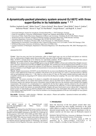
& Tuomi (2012). The algorithm appears to be a well suited to
the fitting of Doppler data in terms of its relatively fast conver-
gence – even when the posterior is not unimodal (Tuomi 2012)
– and it provides samples that represent well the posterior den-
sities. We use these samples to locate the regions of maximum
a posteriori probability in the parameter space and to estimate
each parameter confidence interval allowed by the data. We de-
scribe the parameter densities briefly by using the maximum
a posteriori probability (MAP) estimates as the most probable
values, i.e. our preferred solution, and by calculating the 99%
Bayesian credibility sets (BCSs) surrounding these estimates.
Because of the caveats of point estimates (e.g., inability to de-
scribe the shapes of posterior densities in cases of multimodal-
ity and/or non-negligible skewness), we also plot marginalized
distributions of the parameters that are more important from a
detection and characterization point of view, namely, velocity
semi-amplitudes Kj, and eccentricities ej.
The availability of samples from the posterior densities of
our statistical models also enables us to take advantage of the
signal detection criteria given in Tuomi (2012). To claim that a
signal is a significant one, we require that 1) its period is well-
constrained from above and below, 2) its RV amplitude has a
density that differs from zero significantly (excluded from the
99% credibility intervals), and 3) the posterior probability of the
model containing k+1 signals must be (at least) 150 times greater
than that of the model containing only k signals.
The threshold of 150 on condition (3) might seem arbitrary.
Admitting that posterior probabilities also have uncertainties
(Jenkins & Peacock 2011), we consider that such threshold is
the minimum safe one. As made explicit in the definition of the
posterior density function π(θ|m), the likelihood function is not
the only source of information. We take into account the fact
that all parameter values are not equally probable prior to mak-
ing the measurements via prior probability densities. Essentially,
our priors are chosen as in Tuomi (2012). Of special relevance
in the detection process is the prior choice for the eccentricities.
Our functional choice for it (Gaussian with zero mean and σe =
0.3) is based on statistical, dynamical and population considera-
tions and it is discussed further in the appendices (Appendix A).
For more details on different prior choices, see dedicated discus-
sion in Tuomi & Anglada-Escudé (2013).
4.2. Log–Likelihood periodograms
Because the orbital period (or frequency) is an extremely non-
linear parameter, the orbital solution of a model with k + 1
signals typically contains many hundreds or thousands of local
likelihood maxima (also called independent frequencies). In any
method based on stochastic processes, there is always a chance
that the global maxima of the target function is missed. Our
log–likelihood periodogram (or log–L periodogram) is a tool
to systematically identify periods for new candidate planets of
higher probability and ensure that these areas have been well ex-
plored by the Bayesian samplings (e.g., we always attempt to
start the chains close to the five most significant periodicities
left in the data). A log–L periodogram consists on computing
the improvement of the logarithm of the likelihood (new model
with k + 1 planets) compared to the logarithm of the likelihood
of the null hypothesis (only k planets) at each test period. Log–
L periodograms are represented as period versus ∆ log L plot,
where log is always the natural logarithm. The definition of the
likelihood function we use is in Eq. 2 and typically assumes
Gaussian noise sources only (that is, different jitter parameters
are included for each instrument and g=0 in Eq. 1).
0
20
40
60
80
100
∆logL
0
10
20
30
40
∆logL
0
10
20
30
40
∆logL
0
10
20
∆logL
0
5
10
15
20
∆logL
0
5
10
15
20
∆logL
10 100 1000
Period [days]
0
5
10
∆logL
b
c
d
e
f
g
7.2 days
28.1 days
91 days
62 days
39 days
260 days
17 days?
(h)
(all circular)
Fig. 2. Log–likelihood periodograms for the seven candidate signals
sorted by significance. While the first six signals are easily spotted,
the seventh is only detected with log–L periodograms if all orbits are
assumed to be circular.
∆ log L can also be used for estimating the frequentist false
alarm probability (FAP) of a solution using the likelihood-ratio
test for nested models. This FAP estimates what fraction of
times one would recover such a significant solution by an un-
fortunate arrangement of Gaussian noise. To compute this FAP
from ∆ log L we used the up-to-date recipes provided by Baluev
(2009). We note that that maximization of the likelihood in-
volves solving for many parameters simultaneous: orbital pa-
rameters of the new candidate, all orbital parameters of the al-
ready detected signals, a secular acceleration term ˙γ, a zero-point
γl for each instrument, and jitter terms σl of each instrument
(see Eq. 1). It is, therefore, a computationally intensive task,
especially when several planets are included and several thou-
sand of test periods for the new candidate must be explored. As
discussed in the appendices (see Section A.1), allowing for full
Keplerian solutions at the period search level makes the method
very prone to false positives. Therefore while a full Keplerian
solution is typically assumed for all the already detected k-
candidates, the orbital model for the k + 1-candidate is always
assumed to be circular in our standard setup. This way, our log–L
periodograms represent a natural generalization of more classic
hierarchical periodogram methods. This method was designed
to account for parameter correlations at the detection level. If
such correlations are not accounted for, the significance of new
signals can be strongly biased causing both false positives and
missed detections. In the study of the planet hosting M-dwarf
GJ 676A (Anglada-Escudé & Tuomi 2012) and in the more re-
cent manuscript on GJ 581 (Tuomi & Jenkins 2012), we have
shown that -while log–L periodograms represent an improve-
6

Table 3. Relative posterior probabilities and log-Bayes factors of mod-
els Mk with k Keplerian signals given the combined HARPS-TERRA,
HIRES, and PFS RV data of GJ 667C. Factor ∆ indicates how much
the probability increases with respect to the best model with one less
Keplerian and P denotes the MAP period estimate of the signal added
to the solution when increasing k. Only the highest probability sequence
is shown here (reference solution). A complete table with alternative so-
lutions corresponding to local probability maxima is given in Appendix
B.2
k P(Mk|d) ∆ log P(d|Mk) P [days] ID
0 2.7×10−85
– -602.1 –
1 3.4×10−48
1.3×1037
-516.0 7.2
2 1.3×10−35
3.9×1012
-486.3 91
3 8.9×10−18
6.7×1017
-444.5 28
4 1.9×10−14
2.1×103
-436.2 53
4 1.2×10−14
1.3×103
-436.7 62
5 1.0×10−7
5.5×106
-420.0 39, 53
5 1.0×10−8
5.3×105
-422.3 39, 62
6 4.1×10−3
4.0×104
-408.7 39, 53, 256
6 4.1×10−4
4.0×103
-411.0 39, 62, 256
7 0.057 14 -405.4 17, 39, 53, 256
7 0.939 230 -402.6 17, 39, 62, 256
ment with respect previous periodogram schemes- the afore-
mentioned Bayesian approach has a higher sensitivity to lower
amplitude signals and is less prone to false positive detections.
Because of this, the use of log–L periodograms is not to quantify
the significance of a new signal but to provide visual assessment
of possible aliases or alternative high-likelihood solutions.
Log–L periodograms implicitly assume flat priors for all the
free parameters. As a result, this method provides a quick way of
assessing the sensitivity of a detection against a choice of prior
functions different from uniform. As discussed later, the sixth
candidate is only confidently spotted using log–L periodograms
(our detection criteria is FAP< 1%) when the orbits of all the
candidates are assumed to be circular. This is the red line be-
yond which our detection criteria becomes strongly dependent
on our choice of prior on the eccentricity. The same applies to
the seventh tentative candidate signal.
5. Signal detection and confidences
As opposed to other systems analyzed with the same techniques
(e.g. Tau Ceti or HD 40307, Tuomi et al. 2012, 2013), we found
that for GJ 667C the simplest model (g = 0 in equation 1) al-
ready provides a sufficient description of the data. For brevity,
we omit here all the tests done with more sophisticated param-
eterizations of the noise (see Appendix C) that essentially lead
to unconstrained models for the correlated noise terms and the
same final results. In parallel with the Bayesian detection se-
quence, we also illustrate the search using log–L periodograms.
In all that follows we use the three datasets available at this time :
HARPS-TERRA, HIRES and PFS. We use the HARPS-TERRA
Doppler measurements instead of CCF ones because TERRA
velocities have been proven to be more precise on stable M-
dwarfs (Anglada-Escudé & Butler 2012).
The first three periodicities (7.2 days, 28.1 days and 91 days)
were trivially spotted using Bayesian posterior samplings and
the corresponding log–L periodograms. These three signals were
already reported by Anglada-Escudé et al. (2012) and Delfosse
et al. (2012), although the last one (signal d, at 91 days) remained
uncertain due to the proximity to a characteristic time-scale of
the star’s activity. This signal is discussed in the context of stellar
activity in Section 6. Signal d has a MAP period of 91 days and
would correspond to a candidate planet with a minimum mass of
∼ 5 M⊕.
After that, the log–L periodogram search for a fourth sig-
nal indicates a double-peaked likelihood maximum at 53 and
62 days -both candidate periods receiving extremely low false-
alarm probability estimates (see Figure 2). Using the recipes in
Dawson & Fabrycky (2010), it is easy to show that the two peaks
are the yearly aliases of each other. Accordingly, our Bayesian
samplings converged to either period equally well giving slightly
higher probability to the 53-day orbit (×6). In both cases, we
found that including a fourth signal improved the model proba-
bility by a factor >103
. In appendix B.2 we provide a detailed
analysis and derived orbital properties of both solutions and
show that the precise choice of this fourth period does not sub-
stantially affect the confidence of the rest of the signals. As will
be shown at the end of the detection sequence, the most likely
solution for this candidate corresponds to a minimum mass of
2.7 M⊕ and a period of 62 days.
After including the fourth signal, a fifth signal at 39.0 days
shows up conspicuously in the log–L periodograms. In this case,
the posterior samplings always converged to the same period of
39.0 days without difficulty (signal f). Such planet would have
a minimum mass of ∼2.7 M⊕. Given that the model probability
improved by a factor of 5.3×105
and that the FAP derived from
the log-L periodogram is 0.45%, the presence of this periodicity
is also supported by the data without requiring further assump-
tions.
The Bayesian sampling search for a sixth signal always con-
verged to a period of 260 days that also satisfied our detection
criteria and increased the probability of the model by a 4 × 103
factor. The log–L periodograms did spot the same signal as the
most significant one but assigned a FAP of ∼20% to it. This ap-
parent contradiction is due to the prior on the eccentricity. That
is, the maximum likelihood solution favors a very eccentric orbit
for the Keplerian orbit at 62 days (ee ∼ 0.9), which is unphys-
ical and absorbs variability at long timescales through aliases.
To investigate this, we performed a log–L periodogram search
assuming circular orbits for all the candidates. In this case, the
260-day period received a FAP of 0.5% which would then qual-
ify as a significant detection. Given that the Bayesian detection
criteria are well satisfied and that the log–L periodograms also
provide substantial support for the signal, we also include it in
the model (signal g). Its amplitude would correspond to a mini-
mum mass of 4.6 M⊕.
When performing a search for a seventh signal, the posterior
samplings converged consistently to a global probability maxi-
mum at 17 days (M sin i ∼ 1.1 M⊕) which improves the model
probability by a factor of 230. The global probability maximum
containing seven signals corresponds to a solution with a period
of 62 days for planet e. This solution has a total probability ∼
16 times larger than the one with Pe = 53 days. Although such
difference is not very large to make a final decision on which pe-
riod is preferred, from now on we will assume that our reference
solution is the one with Pe = 62.2 days. The log–L periodogram
also spotted the same seventh period as the next favored one but
only when all seven candidates were assumed to have circular or-
bits. Given that this seventh signal is very close to the Bayesian
detection limit, and based on our experience on the analysis of
similar datasets (e.g., GJ 581 Tuomi & Jenkins 2012), we admit
that this candidate requires more measurements to be securely
confirmed. With a minimum mass of only ∼ 1.1 M⊕, it would be
among the least massive exoplanets to date.
7

Fig. 3. Marginalized posterior densities for the Doppler semi-amplitudes of the seven reported signals.
0 2 4 6
Phase [days]
-9
-6
-3
0
3
6
9
RV[ms
-1
]
b
0 5 10 15 20 25
Phase [days]
-9
-6
-3
0
3
6
9
RV[ms
-1
]
c
0 20 40 60 80
Phase [days]
-9
-6
-3
0
3
6
9
RV[ms
-1
]
d
0 10 20 30 40 50 60
Phase [days]
-9
-6
-3
0
3
6
9
RV[ms
-1
]
e
0 10 20 30
Phase [days]
-9
-6
-3
0
3
6
9
RV[ms
-1
]
f
0 50 100 150 200 250
Phase [days]
-9
-6
-3
0
3
6
9
RV[ms
-1
]
g
0 5 10 15
Phase [days]
-9
-6
-3
0
3
6
9
RV[ms
-1
]
(h)
Fig. 4. RV measurements phase-folded to the best period for each planet. Brown circles are HARPS-TERRA velocities, PFS velocities are depicted
as blue triangles, and HIRES velocities are green triangles. Red squares are averages on 20 phase bins of the HARPS-TERRA velocities. The black
line corresponds to the best circular orbital fit (visualization purposes only).
As a final comment we note that, as in Anglada-Escudé et al.
(2012) and Delfosse et al. (2012), a linear trend was always in-
cluded in the model. The most likely origin of such a trend is
gravitational acceleration caused by the central GJ 667AB bi-
nary. Assuming a minimum separation of 230 AU, the acceler-
ation in the line-of-sight of the observer can be as large as 3.7
m s−1
, which is of the same order of magnitude as the observed
trend of ∼ 2.2 m s−1
yr−1
. We remark that the trend (or part of
it) could also be caused by the presence of a very long period
planet or brown dwarf. Further Doppler follow-up, astrometric
measurements, or direct imaging attempts of faint companions
might help addressing this question.
In summary, the first five signals are easily spotted using
Bayesian criteria and log–L periodograms. The global seven-
Keplerian solution prefers a period of 62.2 days for signal e
which we adopt as our reference solution. Still, a period of 53
days for the same signal cannot be ruled out at the moment. The
statistical significance of a 6th periodicity depends on the prior
choice on the eccentricity, but the Bayesian odds ratio is high
enough to propose it as a genuine Keplerian signal. The statisti-
cal significance of the last seventh candidate (h) is close to our
detection limit and more observations are needed to confirm it.
6. Activity
In addition to random noise (white or correlated), stellar activity
can also generate spurious Doppler periodicities that can mimic
planetary signals (e.g., Lovis et al. 2011; Reiners et al. 2013).
In this section we investigate whether there are periodic varia-
tions in the three activity indices of GJ 667C (S-index, BIS and
FWHM are described in Section 3). Our general strategy is the
following : if a significant periodicity is detected in any of the in-
dices and such periodicity can be related to any of the candidate
signals (same period or aliases), we add a linear correlation term
to the model and compute log–L periodograms and new sam-
plings of the parameter space. If the data were better described
by the correlation term rather than a genuine Doppler signal, the
overall model probability would increase and the planet signal
in question should decrease its significance (even disappear).
Log–L periodogram analysis of two activity indices (S-index
but specially the FWHM) show a strong periodic variability
at 105 days. As discussed in Anglada-Escudé et al. (2012);
Delfosse et al. (2012), this cast some doubt on the candidate at
91 days (d). Despite the fact that the 91-day and 105-day peri-
ods are not connected by first order aliases, the phase sampling
in this period domain is sparse (see phase–folded diagrams of
the RV data for the planet d candidate in Fig. 4) and the log–L
periodogram for this candidate also shows substantial power at
105 days. From the log–L periodograms in Figure 2, one can di-
8

Table 4. Reference orbital parameters and their corresponding 99% credibility intervals. While the angles ω and M0 are unconstrained due to strong degeneracies at small eccentricities,
their sum λ = M0 + ω is better behaved and is also provided here for reference.
b (h) c f e∗
P [days] 7.2004 [7.1987, 7.2021] 16.946 [16.872, 16.997] 28.140 [28.075, 28.193] 39.026 [38.815, 39.220] 62.24 [61.69, 62.79]
e 0.13 [0.02, 0.23] 0.06 [0, 0.38] 0.02 [0, 0.17] 0.03 [0, 0.19] 0.02 [0, 0.24]
K [m s−1
] 3.93 [3.55, 4.35] 0.61 [0.12, 1.05] 1.71 [1.24, 2.18] 1.08 [0.62, 1.55] 0.92 [0.50, 1.40]
ω [rad] 0.10 [5.63, 0.85] 2.0 [0, 2π] 5.1 [0, 2π] 1.8 [0, 2π] 0.5 [0, 2π]
M0 [rad] 3.42 [2.32, 4.60] 5.1 [0, 2π] 0.3 [0, 2π] 5.1 [0, 2π] 4.1 [0, 2π]
λ [deg] 201[168, 250] 45(180)†
308(99)†
34 (170)†
262(150)†
M sin i [M⊕] 5.6 [4.3, 7.0] 1.1 [0.2, 2.1] 3.8 [2.6, 5.3] 2.7 [1.5, 4.1] 2.7 [1.3, 4.3]
a [AU] 0.0505 [0.0452, 0.0549] 0.0893 [0.0800, 0.0977] 0.125 [0.112, 0.137] 0.156 [0.139, 0.170] 0.213 [0.191, 0.232]
d g Other model parameters
P [days] 91.61 [90.72, 92.42] 256.2 [248.3, 270.0] ˙γ [m s−1
yr−1
] 2.07 [1.79, 2.33]
e 0.03 [0, 0.23] 0.08 [0, 0.49] γHARPS [m s−1
] -30.6 [-34.8, -26.8]
K [m s−1
] 1.52 [1.09, 1.95] 0.95 [0.51, 1.43] γHIRES [m s−1
] -31.9 [-37.0,, -26.9]
ω [rad] 0.7 [0, 2π] 0.9 [0, 2π] γPFS [m s−1
] -25.8 [-28.9, -22.5]
M0 [rad] 3.7 [0, 2π] 4.1 [0, 2π] σHARPS [m s−1
] 0.92 [0.63, 1.22]
σHIRES [m s−1
] 2.56 [0.93, 5.15]
λ [deg] 251(126)†
285(170)†
σPFS [m s−1
] 1.31 [0.00, 3.85]
M sin i [M⊕] 5.1 [3.4, 6.9] 4.6 [2.3, 7.2]
a [AU] 0.276 [0.246, 0.300] 0.549 [0.491, 0.601]
Notes. † Values allowed in the full range of λ. Full-width-at-half-maximum of the marginalized posterior is provided to illustrate the most likely
range (see Figure 10). ∗ Due to the presence of a strong alias, the orbital period of this candidate could be 53 days instead. Such alternative orbital
solution for planet e is given in Table B.2.
10 100 1000
0
5
10
15
∆logL
10 100 1000
Period [days]
0
5
10
15
∆logL
dd c ef g(h)
105 days
29 days
S-index (1)
S-index (2)
10 100 1000
0
5
10
15
20
∆logL
10 100 1000
Period [days]
0
5
10
15
∆logL
dd c ef g(h)
FWHM (1)
FWHM (2)
105 days
110 days
Fig. 5. Top two panels Log–L periodograms for up to 2 signals in the
S-index. The most likely periods of the proposed planet candidates are
marked as vertical lines. Bottom two panels. Log–L periodograms for
up to 2 signals in the FWHM. Given the proximity of these two signals,
it is possible that both of them originate from the same feature (active
region corotating with the star) that is slowly evolving with time.
rectly obtain the probability ratio of a putative solution at 91 days
versus one with a period of 105 days when no correlation terms
are included. This ratio is 6.8 × 104
, meaning that the Doppler
period at 91 days is largely favored over the 105-day one. All
10 100 1000
Period [days]
0
10
20
30
40
∆logL
No correlation term
Including correlation term
105 days
91 days
Fig. 6. Log–likelihood periodograms for planet d (91 days) including
the correlation term (red dots) compared to the original periodogram
without them (black line). The inclusion of the correlation term in-
creases the contrast between the peaks at 91 and 105 days, favoring
the interpretation of the 91 days signals as a genuine planet candidate.
Bayesian samplings starting close to the 105-day peak ended-up
converging on the signal at 91 day. We then applied our valida-
tion procedure by inserting linear correlation terms in the model
(g=CF× FWHMi or g=CS × Si), in eq. 1) and computed both
log–L periodograms and Bayesian samplings with CF and CS as
free parameters. In all cases the ∆ log L between 91 and 105 days
slightly increased thus supporting that the signal at 91 days is of
planetary origin. For example, the ratio of likelihoods between
the 91 and the 105 days increased from 6.8×104
to 3.7×106
when
the correlation term with the FWHM was included (see Figure
6). The Bayesian samplings including the correlation term did
not improve the model probability (see Appendix C) and still
preferred the 91-day signal overwhelmingly. We conclude that
this signal is not directly related to the stellar activity and there-
fore is a valid planet candidate.
Given that activity might induce higher order harmonics in
the time-series, all seven candidates have been analyzed and
double-checked using the same approach. Some more details on
the results from the samplings are given in the Appendix C.2. All
candidates -including the tentative planet candidate h- passed all
these validation tests without diﬃculties.
9

Table 5. Most significant periods as extracted using log–L periodograms on subsamples of the first Nobs measurements. Boldfaced values indicate
coincidence with a signal of our seven-planet solution (or a first order yearly alias of it). A parenthesis in the last period indicates preferred period
that did not satisfy the frequentist 1% FAP threshold but did satisfy the Bayesian detectability criteria.
Nobs 1 2 3 4 5 6 7
50 7.2 101.5 – – – – –
75 7.2 103.0 – – – – –
90 7.2 28.0 104.1 – – – –
100 7.2 91.2 28.0 54.4a
– – –
120 7.2 91.6 28.0 – – – –
143 7.2 91.6 28.0 53.6a
35.3a
(260) –
160 7.2 28.1 91.0 38.9 53.4a
275 (16.9)
173 7.2 28.1 91.9 61.9 38.9 260 (16.9)
Notes. a
1 year−1
alias of the preferred period in Table 4.
7. Tests for quasi-periodic signals
Activity induced signals and superposition of several indepen-
dent signals can be a source of confusion and result in detec-
tions of “apparent” false positives. In an attempt to quantify how
much data is necessary to support our preferred global solution
(with seven planets) we applied the log-L periodogram analysis
method to find the solution as a function of the number of data
points. For each dataset, we stopped searching when no peak
above FAP 1% was found. The process was fully automated so
no human-biased intervention could alter the detection sequence.
The resulting detection sequences are show in Table 5. In addi-
tion to observing how the complete seven-planet solution slowly
emerges from the data one can notice that for Nobs <100 the
k = 2 and k = 3 solutions converge to a strong signal at ∼ 100
days. This period is dangerously close to the activity one de-
tected in the FWHM and S-index time-series. To explore what
could be the cause of this feature (perhaps the signature of a
quasi-periodic signal), we examined the Nobs=75 case in more
detail and made a supervised/visual analysis of that subset.
The first 7.2 days candidate could be easily extracted. We
then computed a periodogram of the residuals to figure out if
there were additional signals left in the data. In agreement with
the automatic search, the periodogram of the residuals (bottom
of Figure 7) show a very strong peak at ∼100 days. The peak was
so strong that we went ahead and assessed its significance. It had
a very low FAP (< 0.01%) and also satisfied our Bayesian de-
tectability criteria. We could have searched for additional com-
panions, but let us assume we stop our analysis here. In this case,
we would have concluded that two signals were strongly present
(7.2 days and 100 days). Because of the proximity with a period-
icity in the FWHM-index ( 105 days), we would have expressed
our doubts about the reality of the second signal so only one
planet candidate would have been proposed (GJ 667Cb).
With 228 RV measurements in hand (173 HARPS-TERRA,
21 PFS and 23 from HIRES) we know that such conclusion is
no longer compatible with the data. For example, the second and
third planets are very consistently detected at 28 and 91 days. We
investigated the nature of that 100 days signal using synthetic
subsets of observations as follows. We took our preferred seven-
planet solution and generated the exact signal we would expect
if we only had planet c (28 days) in the first 75 HARPS-TERRA
measurements (without noise). The periodogram of such a noise-
less time-series (top panel in Fig. 7) was very different from the
real one. Then, we sequentially added the rest of the signals.
As more planets were added, the periodogram looked closer to
the one from the real data. This illustrates that we would have
reached the same wrong conclusion even with data with negli-
0
20
40
60
80
100
0
20
40
60
80
100
0
20
40
60
0
20
40
60
80
100
120
0
20
40
60
80
100
120
0
20
40
60
80
16 32 64 128 256
Period [days]
0
10
20
30
40
Power
Real set
+28d
+91d
+63d
+39d
+260d
+17d
Fig. 7. Sequence of periodograms obtained from synthetic noiseless
data generated on the first 75 epochs. The signals in Table 4 were se-
quentially injected from top to bottom. The bottom panel is the peri-
odogram to the real dataset after removing the first 7.2 days planet can-
didate.
gible noise. We also find quite remarkable how well the gen-
eral structure of the periodogram was recovered after adding all
of them (comparing the bottom two panels in Fig. 7). While
this is not a statistical proof of significance, it shows that the
periodogram to the residuals from the 1-planet fit (even with
only 75 RVs measurements) is indeed consistent with the pro-
posed seven-planet solution without invoking the presence of
quasi-periodic signals. This experiment also shows that, until
all stronger signals could be well-decoupled (more detailed in-
vestigation showed this happened at about Nobs ∼ 140), proper
and robust identification of the correct periods was very diffi-
cult. We repeated the same exercise with Nobs=100, 120 and
173 (all HARPS measurements) and obtained identical behav-
ior without exception (see panels in Figure 8). Such an effect is
not new and the literature contains several examples that cannot
be easily explained by simplistic aliasing arguments- e.g., see GJ
581d (Udry et al. 2007; Mayor et al. 2009) and HD 125612b/c
(Anglada-Escudé et al. 2010; Lo Curto et al. 2010). The fact that
all signals detected in the velocity data of GJ 667C have similar
10

0
20
40
60
80
100
0
20
40
60
80
0
10
20
30
40
50
0
10
20
30
40
50
0
10
20
30
40
0
10
20
30
40
16 32 64 128 256
Period [days]
0
5
10
15
20
25
Power
Real set
+28d
+91d
+63d
+39d
+260d
+17d
0
20
40
60
80
100
0
20
40
60
80
100
0
10
20
30
40
50
60
70
0
10
20
30
40
50
60
0
10
20
30
40
50
0
10
20
30
40
50
16 32 64 128 256
Period [days]
0
5
10
15
20
25
30
Power
Real set
+28d
+91d
+63d
+39d
+260d
+17d
0
20
40
60
80
100
0
20
40
60
80
0
10
20
30
40
50
0
10
20
30
40
50
0
10
20
30
40
0
10
20
30
40
16 32 64 128 256
Period [days]
0
5
10
15
20
25
30
Power
Real set
+28d
+91d
+63d
+39d
+260d
+17d
Fig. 8. Same as 7 but using the first 100 epochs (left), first 120 (center) and all of them (right).
0
50
100
150
200
∆logL
0
15
30
45
60
∆logL
0
10
20
30
∆logL
0
5
10
15
20
∆logL
0
10
20
30
∆logL
0
5
10
15
20
∆logL
1 10 100 1000
Period [days]
0
5
10
15
20
∆logL
1 10 100 1000
Period [days]
b
c
d
e
f
g
(h)
First half Second half
Fig. 9. Periodograms on first and second half of the time series as obtained when all signals except one were removed from the data. Except
for signal h, all signals are significantly present in both halves and could have been recovered using either half if they had been in single planet
systems.
amplitudes – except perhaps candidate b which has a consider-
ably higher amplitude – made this problem especially severe. In
this sense, the currently available set of observation are a sub–
sample of the many more that might be obtained in the future,
so it might happen that one of the signals we report “bifurcates”
into other periodicities. This experiment also suggests that spec-
tral information beyond the most trivial aliases can be used to
verify and assess the significance of future detections (under in-
vestigation).
7.1. Presence of individual signals in one half of the data
As an additional verification against quasi-periodicity, we inves-
tigated if the signals were present in the data when it was divided
in two halves. First half corresponds to the first 86 HARPS ob-
servations and the second half covers the rest. The data from PFS
and HIRES was not used for this test. The experiment consists in
removing all signals except for one of them at a time and com-
pute the periodogram on those residuals (first and second halfs
separately). If a signal is strongly present in both halfs, it should,
at least, emerge as substantially significant. All signals except for
the seventh one passed this test nicely. That is, in all cases except
for h, the periodograms prominently display the non-removed
11

signal unambiguously. Besides demonstrating that all signals are
strongly present in the two halves, it also illustrates that any
of the candidates would have been trivially spotted using peri-
odograms if it had been orbiting alone around the star. The fact
that each signal was not spotted before (Anglada-Escudé et al.
2012; Delfosse et al. 2012) is a consequence of an inadequate
treatment of signal correlations when dealing with periodograms
of the residuals only. Both the described Bayesian method and
the log-likelihood periodogram technique are able to deal with
such correlations by identifying the combined global solution
at the period search level. As for other multiplanet systems de-
tected using similar techniques (Tuomi et al. 2013; Anglada-
Escudé & Tuomi 2012), optimal exploration of the global proba-
bility maxima at signal search level is essential to properly detect
and assess the significance of low mass multiplanet solutions,
especially when several signals have similar amplitudes close to
the noise level of the measurements.
Summarizing these investigations and validation of the sig-
nals against activity, we conclude that
– Up to seven periodic signals are detected in the Doppler mea-
surements of GJ 667C data, being the last (seventh) signal
very close to our detection threshold.
– The significance of the signals is not affected by correlations
with activity indices and we could not identify any strong
wavelength dependence with any of them.
– The first six signals are strongly present in subsamples of
the data. Only the seventh signal is unconfirmed using half
of the data only. Our analysis indicates that any of the six
stronger signals would had been robustly spotted with half
the available data if each had been orbiting alone around the
host star.
– Signal correlations in unevenly sampled data is the reason
why Anglada-Escudé et al. (2012) and Delfosse et al. (2012)
only reported three of them. This is a known problem as-
sessing the significance of signals when using periodograms
of residuals only (see Anglada-Escudé & Tuomi 2012, as
another example).
Given the results of these validation tests, we promote six of the
signals (b, c, d, e, f, g) to planet candidates. For economy of
language, we will refer to them as planets but the reader must
remember that, unless complementary and independent verifica-
tion of a Doppler signal is obtained (e.g., transits), they should be
called planet candidates. Verifying the proposed planetary sys-
tem against dynamical stability is the purpose of the next section.
8. Dynamical analysis
One of the by-products of the Bayesian analysis described in the
previous sections, are numerical samples of statistically allowed
parameter combinations. The most likely orbital elements and
corresponding confidence levels can be deduced from these sam-
ples. In Table 4 we give the orbital configuration for a planetary
system with seven planets around GJ 667C, which is preferred
from a statistical point of view. To be sure that the proposed
planetary system is physically realistic, it is necessary to confirm
that these parameters not only correspond to the solution favored
by the data, but also constitute a dynamically stable configura-
tion. Due to the compactness of the orbits, abundant resonances
and therefore complex interplanetary interactions are expected
within the credibility intervals. To slightly reduce this complex-
ity and since evidence for planet h is weak, we split our analysis
and present in the first part of this section the results for the six-
planet solution with planets b to g. The dynamical feasibility of
the seven-planet solution is then assessed by investigating the
semi-major axis that would allow introducing a seventh planet
with the characteristics of planet h.
8.1. Finding stable solutions for six planets
A first thing to do is to extract from the Bayesian samplings
those orbital configurations that allow stable planetary motion
over long time scales, if any. Therefore we tested the stability of
each configuration by a separate numerical integration using the
symplectic integrator SABA2 of Laskar & Robutel (2001) with
a step size τ = 0.0625 days. In the integration we included a cor-
rection term to account for general relativistic precession. Tidal
effects were neglected for these runs. Possible effects of tides are
discussed separately in Section 9.4. The integration was stopped
if any of the planets went beyond 5 AU or planets approached
each other closer than 10−4
AU.
The stability of those configurations that survived the inte-
gration time span of 104
orbital periods of planet g (i. e. ≈ 7000
years), was then determined using frequency analysis (Laskar
1993). For this we computed the stability index Dk for each
planet k as the relative change in its mean motion nk over two
consecutive time intervals as was done in Tuomi et al. (2013).
For stable orbits the computed mean motion in both intervals
will be almost the same and therefore Dk will be very small. We
note that, that this also holds true for planets captured inside a
mean-motion resonance (MMR), as long as this resonance helps
to stabilize the system. As an index for the total stability of a con-
figuration we used D = max(|Dk|). The results are summarized
in Figure 10. To generate Figure 10, we extracted a sub-sample
of 80,000 initial conditions from the Bayesian samplings. Those
configurations that did not reach the final integration time are
represented as gray dots. By direct numerical integration of the
remaining initial conditions we found that almost all configura-
tions with D < 10−5
survive a time span of 1 Myr. This corre-
sponds to ∼0.3 percent of the total sample. The most stable orbits
we found (D < 10−6
) are depicted as black crosses.
In Figure 10 one can see that the initial conditions taken from
the integrated 80,000 solutions are already confined to a very
narrow range in the parameter space of all possible orbits. This
means, that the allowed combinations of initial a and λ are al-
ready quite restricted by the statistics. By examining Figure 10
one can also notice that those initial conditions that turned out
to be long-term stable are quite spread along the areas where
the density of Bayesian states is higher. Also, for some of the
candidates, (d, f and g) and d) there are regions were no orbit
was found with D<10−5
. The paucity of stable orbits at certain
regions indicate areas of strong chaos within the statistically al-
lowed ranges (likely disruptive mean-motion resonances) and il-
lustrate that the dynamics of the system are far from trivial.
The distributions of eccentricities are also strongly affected
by the condition of dynamical stability. In Figure 11 we show
the marginalized distributions of eccentricities for the sample
of all the integrated orbits (gray histograms) and the distribu-
tion restricted to relatively stable orbits (with D< 10−5
, red his-
tograms). We see that, as expected, stable motion is only pos-
sible with eccentricities smaller than the mean values allowed
by the statistical samples. The only exceptions are planets b
and g. These two planet candidates are well separated from the
other candidates. As a consequence, their probability densities
are rather unaffected by the condition of long-term stability. We
note here that the information about the dynamical stability has
been used only a posteriori. If we had used long-term dynamics
as a prior (e.g., assign 0 probability to orbits with D>10−5
), mod-
12

0.050425 0.05043 0.050435 0.05044
0
90
180
270
360
λ[deg]
0.1249 0.1250 0.1251 0.1252 0.1253
0.211 0.212 0.213 0.214 0.215
a [au]
0
90
180
270
360
λ[deg]
0.273 0.274 0.275 0.276 0.277
0.155 0.1555 0.156 0.1565
a [au]
0.536 0.544 0.552
a [au]
b c d
e f g
Fig. 10. Result of the stability analysis of 80,000 six-planet solutions in the plane of initial semi-major axis a vs. initial mean longitude λ obtained
from a numerical integration over T ≈ 7000 years. Each initial condition is represented as a point. Initial conditions leading to an immediate
disintegration of the system are shown as gray dots. Initial conditions that lead to stable motion for at least 1 Myr are shown as red points
(D< 10−5
). Black crosses represent the most stable solutions (D< 10−6
), and can last over many Myr.
Table 6. Astrocentric orbital elements of solution S6.
Planet P (d) a (AU) e ω (◦
) M0 (◦
) M sin i (M⊕)
b 7.2006 0.05043 0.112 4.97 209.18 5.94
c 28.1231 0.12507 0.001 101.38 154.86 3.86
f 39.0819 0.15575 0.001 77.73 339.39 1.94
e 62.2657 0.21246 0.001 317.43 11.32 2.68
d 92.0926 0.27580 0.019 126.05 243.43 5.21
g 251.519 0.53888 0.107 339.48 196.53 4.41
erately eccentric orbits would have been much more strongly
suppressed than with our choice of prior function (Gaussian dis-
tribution of zero mean and σ = 0.3, see Appendix A.1). In this
sense, our prior density choice provides a much softer and unin-
formative constraint than the dynamical viability of the system.
In the following we will use the set of initial conditions that
gave the smallest D for a detailed analysis and will refer to it
as S6. In Table 6, we present the masses and orbital parameters
of S6, and propose it as the favored configuration. To double
check our dynamical stability results, we also integrated S6 for
108
years using the HNBody package (Rauch & Hamilton 2002)
including general relativistic corrections and a time step of τ =
10−3
years.1
8.2. Secular evolution
Although the dynamical analysis of such a complex system with
different, interacting resonances could be treated in a separate
paper, we present here some basic analysis of the dynamical ar-
1
Publicly available at http://janus.astro.umd.edu/HNBody/
chitecture of the system. From studies of the Solar System we
know that, in the absence of mean motion resonances, the vari-
ations in the orbital elements of the planets are governed by the
so-called secular equations. These equations are obtained after
averaging over the mean longitudes of the planets. Since the
involved eccentricities for GJ 667C are small, the secular sys-
tem can be limited here to its linear version, which is usually
called Laplace-Lagrange solution (for details see Laskar (1990)).
Basically, the solution is obtained from a transformation of the
complex variables zk = ekeıϖk
into the proper modes uk. Here ek
are the eccentricities and ϖk the longitudes of the periastron of
planet k = b, c, . . . , g. The proper modes uk determine the secular
variation of the eccentricities and are given by uk ≈ ei(gkt+ϕk)
.
Since the transformation into the proper modes depends only
on the masses and semi-major axes of the planets, the secular
frequencies will not change much for the different stable config-
urations found in Figure 10. Here we use solution S6 to obtain
numerically the parameters of the linear transformation by a fre-
quency analysis of the numerically integrated orbit. The secular
frequencies gk and the phases ϕk are given in Table 7. How well
13

0 0.1 0.2 0.3 0.4 0.5
eb
0
0.1
0.2
0.3
0.4
0.5
Frequency
0 0.1 0.2 0.3 0.4 0.5
ec
0
0.1
0.2
0.3
0.4
0.5
Frequency
0 0.1 0.2 0.3 0.4 0.5
ed
0
0.1
0.2
0.3
0.4
0.5
Frequency
0 0.1 0.2 0.3 0.4 0.5
ee
0
0.1
0.2
0.3
0.4
0.5
Frequency
0 0.1 0.2 0.3 0.4 0.5
ef
0
0.1
0.2
0.3
0.4
0.5
Frequency
0 0.1 0.2 0.3 0.4 0.5
eg
0
0.1
0.2
0.3
0.4
0.5
Frequency
Fig. 11. Marginalized posterior densities for the orbital eccentricities of the six planet solution (b, c, d, in the first row; e, f, g in the second) before
(gray histogram) and after (red histogram) ruling out dynamically unstable configuration.
0
0.02
0.04
0.06
0.08
0.1
0.12
5000 7500 10000 12500
eccentricity
t [yr]
b
c
f
e
d
g
Fig. 12. Evolution of the eccentricities of solution S6. Colored lines give
the eccentricity as obtained from a numerical integration. The thin black
lines show the eccentricity of the respective planet as given by the lin-
ear, secular approximation. Close to each line we give the name of the
corresponding planet.
the secular solution describes the long-term evolution of the ec-
centricities can be readily seen in Figure 12.
Table 7. Fundamental secular frequencies gk, phases ϕk and correspond-
ing periods of the six-planet solution.
k gk ϕk Period
[deg/yr] [deg] [yr]
1 0.071683 356.41 5022.09
2 0.184816 224.04 1947.88
3 0.991167 116.46 363.21
4 0.050200 33.63 7171.37
5 0.656733 135.52 548.17
6 0.012230 340.44 29435.80
From Figure 12, it is easy to see that there exists a strong sec-
ular coupling between all the inner planets. From the Laplace-
Lagrange solution we find that the long-term variation of the
eccentricities of these planets is determined by the secular fre-
quency g1 −g4 with a period of ≈ 17000 years. Here the variation
in eccentricity of planet b is in anti-phase to that of planets c to
f due to the exchange of orbital angular momentum. On shorter
time scales we easily spot in Figure 12 the coupling between
planets d and e with a period of ≈ 600 years (g1 − g5), while
the eccentricities of planets c and f vary with a period of almost
3000 years (g1 + g4). Such couplings are already known to pre-
vent close approaches between the planets (Ferraz-Mello et al.
2006). As a result, the periastron of the planets are locked and
the difference ∆ϖ between any of their ϖ librates around zero.
Although the eccentricities show strong variations, these
changes are very regular and their maximum values remain
bounded. From the facts that 1) the secular solution agrees so
well with numerically integrated orbits, and 2) at the same time
the semi-major axes remain nearly constant (Table 8), we can
conclude that S6 is not affected by strong MMRs.
Nevertheless, MMRs that can destabilize the whole system
are within the credibility intervals allowed by the samplings and
not far away from the most stable orbits. Integrating some of the
initial conditions marked as chaotic in Figure 10 one finds that,
for example, planets d and g are in some of these cases temporar-
ily trapped inside a 3:1 MMR, causing subsequent disintegration
of the system.
Table 8. Minimum and maximum values of the semi-major axes and
eccentricities during a run of S6 over 10 Myr.
k amin amax emin emax
b 0.050431 0.050433 0.035 0.114
c 0.125012 0.125135 0.000 0.060
f 0.155582 0.155922 0.000 0.061
e 0.212219 0.212927 0.000 0.106
d 0.275494 0.276104 0.000 0.087
g 0.538401 0.539456 0.098 0.116
8.3. Including planet h
After finding a non-negligible set of stable six-planet solutions, it
is tempting to look for more planets in the system. From the data
analysis one even knows the preferred location of such a planet.
We first considered doing an analysis similar to the one for the
six-planet case using the Bayesian samples for the seven-planet
solution. As shown in previous sections, the subset of stable so-
14

0.05 0.1 0.15 0.2
a [AU]
0
0.05
0.1
0.15
eccentricity
-6
-5
-4
-3
max|Dk|
b
h
c f
Fig. 13. Stability plot of the possible location of a 7th planet in the sta-
ble S6 solution (Table 5). We investigate the stability of an additional
planet with 1.1 Earth masses around the location found by the Bayesian
analysis. For these integrations we varied the semi-major axis and ec-
centricity of the putative planet on a regular grid. The orbital angles
ω and M0 were set to the values of the statistically preferred solution,
while the inclination was fixed to zero. The nominal positions of the
planets as given in Table 6 are marked with white crosses.
lutions found by this approach is already small compared to the
statistical samples in the six-planet case (∼ 0.3%). Adding one
more planet (five extra dimensions) can only shrink the relative
volume of stable solutions further. Given the large uncertainties
on the orbital elements of h, we considered this approach too
computationally expensive and inefficient.
As a first approximation to the problem, we checked whether
the distances between neighboring planets are still large enough
to allow stable motion. In Chambers et al. (1996) the mean life-
time for coplanar systems with small eccentricities is estimated
as a function of the mutual distance between the planets, their
masses and the number of planets in the system. From their re-
sults we can estimate the expected lifetime for the seven planet
solution to be at least 108
years.
Motivated by this result, we explored the phase space around
the proposed orbit for the seventh planet. To do this, we use solu-
tion S6 and placed a fictitious planet with 1.1 M⊕ (the estimated
mass of planet h as given in Table 4) in the semi-major axis range
between 0.035 and 0.2 AU (step size of 0.001 AU) varying the
eccentricity between 0 and 0.2 (step size of 0.01). The orbital an-
gles ω and M0 were set to the values of the statistically preferred
solution for h (see Table 4). For each of these initial configu-
ration we integrated the system for 104
orbits of planet g and
analyzed stability of the orbits using the same secular frequency
analysis. As a result, we obtained a value of the chaos index D
at each grid point. Figure 13 shows that the putative orbit of h
appears right in the middle of the only island of stability left in
the inner region of the system. By direct numerical integration
of solution S6 together with planet h at its nominal position, we
found that such a solution is also stable on Myr timescales. With
this we conclude that the seventh signal detected by the Bayesian
analysis also belongs to a physically viable planet that might be
confirmed with a few more observations.
8.4. An upper limit for the masses
Due to the lack of reported transit, only the minimum masses are
known for the planet candidates. The true masses depend on the
unknown inclination i of the system to the line-of-sight. In all the
analysis presented above we implicitly assume that the GJ 667C
is observed edge-on (i = 90◦
) and that all true masses are equal
to the minimum mass Msin i. As shown in the discussion on the
dynamics, the stability of the system is fragile in the sense that
dynamically unstable configurations can be found close in the
parameter space to the stable ones. Therefore, it is likely that a
more complete analysis could set strong limitations on the max-
imum masses allowed to each companion. An exploration of the
total phase space including mutual inclinations would require
too much computational resources and is beyond the scope of
this paper. To obtain a basic understanding of the situation, we
only search for a constrain on the maximum masses of the S6
solution assuming co-planarity. Decreasing the inclination of the
orbital plane in steps of 10◦
, we applied the frequency analysis
to the resulting system. By making the planets more massive, the
interactions between them become stronger, with a correspond-
ing shrinking of the areas of stability. In this experiment, we
found that the system remained stable for at least one Myr for
an inclination down to i = 30◦
. If this result can be validated by
a much more extensive exploration of the dynamics and longer
integration times (in prep.), it would confirm that the masses of
all the candidates are within a factor of 2 of the minimum masses
derived from Doppler data. Accordingly, c,f and e would be the
first dynamically confirmed super-Earths (true masses below 10
M⊕) in the habitable zone of a nearby star.
9. Habitability
Planets h–d receive 20–200% of the Earth’s current insolation,
and hence should be evaluated in terms of potential habitability.
Traditionally, analyses of planetary habitability begin with deter-
mining if a planet is in the habitable zone (Dole 1964; Hart 1979;
Kasting et al. 1993; Selsis et al. 2007; Kopparapu et al. 2013),
but many factors are relevant. Unfortunately, many aspects can-
not presently be determined due to the limited characterization
derivable from RV observations. However, we can explore the
issues quantitatively and identify those situations in which hab-
itability is precluded, and hence determine which of these plan-
ets could support life. In this section we provide a preliminary
analysis of each potentially habitable planet in the context of pre-
vious results, bearing in mind that theoretical predictions of the
most relevant processes cannot be constrained by existing data.
9.1. The Habitable Zone
The HZ is defined at the inner edge by the onset of a “moist
greenhouse,” and at the outer edge by the “maximum green-
house” (Kasting et al. 1993). Both these definitions assume that
liquid surface water is maintained under an Earth-like atmo-
sphere. At the inner edge the temperature near the surface be-
comes large enough that water cannot be confined to the sur-
face and water vapor saturates the stratosphere. From there, stel-
lar radiation can dissociate the water and hydrogen can escape.
Moreover, as water vapor is a greenhouse gas, large quantities in
the atmosphere can heat the surface to temperatures that forbid
the liquid phase, rendering the planet uninhabitable. At the outer
edge, the danger is global ice coverage. While greenhouse gases
like CO2 can warm the surface and mitigate the risk of global
glaciation, CO2 also scatters starlight via Rayleigh scattering.
15

Fig. 14. Tidal evolution of the spin properties of planet GJ 667C f. Solid lines depict predictions from constant-time-lag theory (“CTL”), while
dashed lines illustrate those from a constant-phase-lag model (“CPL”). All tracks assume a scenario similar to the “base” configuration (see text
and Table 9). Left: Despinning for an assumed initial rotation period of one day. The CPL model yields tidal locking in less than 5 Myr, and CTL
theory predicts about 20 Myr for tidal locking. Right: Tilt erosion of an assumed initial Earth-like obliquity of 23.5◦
. Time scales for both CPL and
CTL models are similar to the locking time scales.
There is therefore a limit to the amount of CO2 that can warm
a planet as more CO2 actually cools the planet by increasing its
albedo, assuming a moist or runaway greenhouse was never trig-
gered.
We use the most recent calculations of the HZ (Kopparapu
et al. 2013) and find, for a 1 Earth-mass planet, that the inner
and outer boundaries of the habitable zone for GJ 667C lie be-
tween 0.095–0.126 AU and 0.241–0.251 AU respectively. We
will adopt the average of these limits as a working definition of
the HZ: 0.111 – 0.246 AU. At the inner edge, larger mass plan-
ets resist the moist greenhouse and the HZ edge is closer in, but
the outer edge is almost independent of mass. Kopparapu et al.
(2013) find that a 10 M⊕ planet can be habitable 5% closer to
the star than a 1 M⊕ planet. However, we must bear in mind that
the HZ calculations are based on 1-dimensional photochemical
models that may not apply to slowly rotating planets, a situation
likely for planets c, d, e, f and h (see below).
From these definitions, we find that planet candidate h (a =
0.0893 AU) is too hot to be habitable, but we note its semi-major
axis is consistent with the most optimistic version of the HZ.
Planet c (a = 0.125 AU) is close to the inner edge but is likely to
be in the HZ, especially since it has a large mass. Planets f and
e are firmly in the HZ. Planet d is likely beyond the outer edge
of the HZ, but the uncertainty in its orbit prevents a definitive
assessment. Thus, we conclude that planets c, f, and e are in
the HZ, and planet d might be, i.e. there up to four potentially
habitable planets orbiting GJ 667C.
Recently, Abe et al. (2011) pointed out that planets with
small, but non-negligible, amounts of water have a larger HZ
than Earth-like planets. From their definition, both h and d are
firmly in the HZ. However, as we discuss below, these planets
are likely water-rich, and hence we do not use the Abe et al.
(2011) HZ here.
9.2. Composition
Planet formation is a messy process characterized by scatter-
ing, migration, and giant impacts. Hence precise calculations of
planetary composition are presently impossible, but see Bond
et al. (2010); Carter-Bond et al. (2012) for some general trends.
For habitability, our first concern is discerning if a planet is
rocky (and potentially habitable) or gaseous (and uninhabitable).
Unfortunately, we cannot even make this rudimentary evaluation
based on available data and theory. Without radii measurements,
we cannot determine bulk density, which could discriminate be-
tween the two. The least massive planet known to be gaseous is
GJ 1214 b at 6.55 M⊕ (Charbonneau et al. 2009), and the largest
planet known to be rocky is Kepler-10 b at 4.5 M⊕ (Batalha
et al. 2011). Modeling of gas accretion has found that planets
smaller than 1 M⊕ can accrete hydrogen in certain circumstances
(Ikoma et al. 2001), but the critical mass is likely larger (Lissauer
et al. 2009). The planets in this system lie near these masses,
and hence we cannot definitively say if any of these planets are
gaseous.
Models of rocky planet formation around M dwarfs have
found that those that accrete from primordial material are likely
to be sub-Earth mass (Raymond et al. 2007) and volatile-
poor (Lissauer 2007). In contrast, the planets orbiting GJ 667C
are super-Earths in a very packed configuration summing up to
> 25 M⊕ inside 0.5 AU. Therefore, the planets either formed at
larger orbital distances and migrated in (e.g. Lin et al. 1996),
or additional dust and ice flowed inward during the protoplan-
etary disk phase and accumulated into the planets Hansen &
Murray (2012, 2013). The large masses disfavor the first sce-
nario, and we therefore assume that the planets formed from ma-
terial that condensed beyond the snow-line and are volatile rich.
If not gaseous, these planets contain substantial water content,
which is a primary requirement for life (and negates the dry-
world HZ discussed above). In conclusion, these planets could
be terrestrial-like with significant water content and hence are
potentially habitable.
9.3. Stellar Activity and habitability
Stellar activity can be detrimental to life as the planets can be
bathed in high energy photons and protons that could strip the
atmosphere or destroy ozone layers. In quiescence, M dwarfs
emit very little UV light, so the latter is only dangerous if flares
occur frequently enough that ozone does not have time to be
replenished (Segura et al. 2010). As already discussed in Section
2, GJ 667C appears to be relatively inactive (indeed, we would
not have been able to detect planetary signals otherwise), and
16

so the threat to life is small today. If the star was very active
in its youth- with mega-flares like those on the equal mass star
AD Leo (Hawley & Pettersen 1991)- any life on the surface of
planets might have been difficult during those days (Segura et al.
2010). While M dwarfs are likely to be active for much longer
time than the Sun (West et al. 2008; Reiners & Mohanty 2012),
GJ 667C is not active today and there is no reason to assume that
life could not form after an early phase of strong stellar activity.
9.4. Tidal Effects
Planets in the HZ of low mass stars may be subject to strong
tidal distortion, which can lead to long-term changes in orbital
and spin properties (Dole 1964; Kasting et al. 1993; Barnes et al.
2008; Heller et al. 2011), and tidal heating (Jackson et al. 2008;
Barnes et al. 2009, 2012). Both of these processes can affect hab-
itability, so we now consider its effects on planets c, d, e, f and
h.
Tides will first spin-lock the planetary spin and drive the
obliquity to either 0 or π. The timescale for these processes
is a complex function of orbits, masses, radii and spins, (see
e.g. Darwin 1880; Hut 1981; Ferraz-Mello et al. 2008; Leconte
et al. 2010) but for super-Earths in the HZ of ∼ 0.3 M⊙, Heller
et al. (2011) found that tidal locking should occur in 106
–109
years. We have used both the constant-time-lag and constant-
phase-lag tidal models described in Heller et al. (2011) and
Barnes et al. (2012) (see also Ferraz-Mello et al. 2008; Leconte
et al. 2010), to calculate how long tidal locking could take for
these planets. We consider two possibilities. Our baseline case
is very similar to that of Heller et al. (2011) in which the plan-
ets initially have Earth-like properties: 1 day rotation period, an
obliquity of 23.5◦
and the current tidal dissipation of the Earth (a
tidal Q of 12-Yoder (1995) or time lag of 638 s-Lambeck (1977);
Neron de Surgy & Laskar (1997)). We also consider an extreme,
but plausible, case that maximizes the timescale for tidal lock-
ing: 8 hour rotation period, obliquity of 89.9◦
and a tidal Q of
1000 or time lag of 6.5 s. In Table 9 we show the time for the
obliquity to erode to 1◦
, tero, and the time to reach the pseudo-
synchronous rotation period, tlock.
In Figure 14, we depict the tidal evolution of the rotation pe-
riod (left panel) and obliquity (right panel) for planet f as an ex-
ample. The assumed initial configuration is similar to the “base”
scenario. Time scales for rotational locking and tilt erosion are
similar to those shown in Table 9.2
As these planets are on nearly circular orbits, we ex-
pect tidally-locked planets to be synchronously rotating, al-
though perhaps when the eccentricity is relatively large pseudo-
synchronous rotation could occur (Goldreich 1966; Murray &
Dermott 1999; Barnes et al. 2008; Correia et al. 2008; Ferraz-
Mello et al. 2008; Makarov & Efroimsky 2013). From Table
9 we see that all the planets h–f are very likely synchronous
rotators, planet e is likely to be, but planet d is uncertain.
Should these planets have tenuous atmospheres (< 0.3 bar), then
they may not support a habitable surface (Joshi et al. 1997).
Considerable work has shown that thicker atmospheres are able
to redistribute dayside heat to produce clement conditions (Joshi
et al. 1997; Joshi 2003; Edson et al. 2011; Pierrehumbert 2011;
Wordsworth et al. 2011). As we have no atmospheric data, we
2
Note that evolution for the CPL model is faster with our parameter-
ization. In the case of Gl581 d, shown in Heller et al. (2011), the planet
was assumed to be less dissipative in the CPL model (Qp = 100) and
evolution in the CPL model was slower.
assert that tidal locking does not preclude habitability for any of
the HZ planets.
During the tidal despinning, tidal heat can be generated as
dissipation transforms rotational energy into frictional heat. In
some cases, the heating rates can be large enough to trigger a
runaway greenhouse and render a planet uninhabitable (Barnes
et al. 2012). Tidal heating is maximized for large radius planets
that rotate quickly and at high obliquity. Using the Leconte et al.
(2010) model and the Earth’s dissipation, we find that tidal heat-
ing of the HZ planets will be negligible for most cases. Consider
an extreme version of planet h, which is just interior to the HZ.
Suppose it has the same tidal dissipation as the Earth (which is
the most dissipative body known), a rotation period of 10 hr, an
eccentricity of 0.1, and an obliquity of 80◦
. The Leconte et al.
(2010) model predicts such a planet would have a tidal heat
flux of nearly 4000 W m−2
. However, that model also predicts
the flux would drop to only 0.16 W m−2
in just 106
years. The
timescale for a runaway greenhouse to sterilize a planet is on the
order of 108
years (Watson et al. 1981; Barnes et al. 2012), so
this burst of tidal heating does not forbid habitability.
After tidal locking, the planet would still have about 0.14 W
m−2
of tidal heating due to the eccentricity (which, as for the
other candidates, can oscillate due to dynamical interactions be-
tween 0 and 0.1). If we assume an Earth-like planet, then about
90% of that heat is generated in the oceans, and 10% in the rocky
interior. Such a planet would have churning oceans, and about
0.01 W m−2
of tidal heat flux from the rocky interior. This num-
ber should be compared to 0.08 W m−2
, the heat flux on the Earth
due entirely to other sources. As e = 0.1 is near the maximum of
the secular cycle, see § 8, the actual heat flux is probably much
lower. We conclude that tidal heating on planet h is likely to be
negligible, with the possibility it could be a minor contributor to
the internal energy budget. As the other planets are more distant,
the tidal heating of those planets is negligible. The CPL predicts
higher heating rates and planet c could receive ∼ 0.01 W m−2
of
internal heating, but otherwise tidal heating does not affect the
HZ planets.
9.5. The Weather Forecast
Assuming planets c, f and e have habitable surfaces (see Figure
15), what might their climates be like? To first order we ex-
pect the planet’s surface temperatures to be cooler as semi-major
axis increases because the incident flux falls off with distance
squared. However, albedo variations can supersede this trend,
e.g. a closer, high-albedo planet could absorb less energy than a
more distant low-albedo planet. Furthermore, molecules in the
atmosphere can trap photons near the surface via the greenhouse
effect, or scatter stellar light via Rayleigh scattering, an anti-
greenhouse effect. For example, the equilibrium temperature of
Venus is actually lower than the Earth’s due to the former’s large
albedo, yet the surface temperature of Venus is much larger than
the Earth’s due to the greenhouse effect.Here we speculate on
the climates of each HZ planet based on the our current under-
standing of the range of possible climates that HZ planets might
have.
Certain aspects of each planet will be determined by the red-
der spectral energy distribution of the host star. For example, the
“stratosphere” is expected to be isothermal as there is negligi-
ble UV radiation (Segura et al. 2003). On Earth, the UV light
absorbed by ozone creates a temperature inversion that delin-
eates the stratosphere. HZ calculations also assume the albedo of
planets orbiting cooler stars are lower than the Earth’s because
Rayleigh scattering is less effective for longer wavelengths, and
17

CPL CTL
base max base max
tlock tero tlock tero tlock tero tlock tero
h 0.07 0.08 18.2 20.4 0.55 0.77 66.9 103
c 0.62 0.69 177 190 4.7 8.1 704 1062
f 2.2 2.3 626 660 18.5 30.1 2670 3902
e 14.2 15.0 4082 4226 129 210 > 104
> 104
d 70.4 73 > 104
> 104
692 1094 > 104
> 104
Table 9. Timescales for the planets’ tidal despinning in units of Myr. “CPL” denotes the constant-phase-lag model of Ferraz-Mello et al. (2008),
“CTL” labels the constant-time-lag model of Leconte et al. (2010).
Fig. 15. Liquid water habitable zone of GJ 667C with the proposed seven candidates as estimated using updated relations in Kopparapu et al.
(2013). Three of the reported planets lie within the HZ. The newly reported planets f and e are the most comfortably located within it. The inner
edge is set by the moist greenhouse runaway limit and the outer edge is set by the snow ball runaway limit. The empirical limits set by a recent
uninhabitable Venus and an early habitable Mars are marked in brown solid lines. The presence of clouds of water (inner edge) or CO2 (outer
edge) might allow habitable conditions on planets slightly outside the nominal definition of the habitable zone (Selsis et al. 2007).
because the peak emission in the stellar spectrum is close to
several H2O and CO2 absorption bands in the near infrared.
Therefore, relative to the Earth’s insolation, the HZ is farther
from the star. In other words, if we placed the Earth in orbit
around an M dwarf such that it received the same incident radia-
tion as the modern Earth, the M dwarf planet would be hotter as
it would have a lower albedo. The different character of the light
can also impact plant life, and we might expect less productive
photosynthesis (Kiang et al. 2007), perhaps relying on pigments
such as chlorophyll d (Mielke et al. 2013) or chlorophyll f (Chen
et al. 2010).
Planet c is slightly closer to the inner edge of the HZ than
the Earth, and so we expect it to be warmer than the Earth, too.
It receives 1230 W m−2
of stellar radiation, which is actually
less than the Earth’s solar constant of 1360 W m−2
. Assuming
synchronous rotation and no obliquity, then the global climate
depends strongly on the properties of the atmosphere. If the at-
mosphere is thin, then the heat absorbed at the sub-stellar point
cannot be easily transported to the dark side or the poles. The
surface temperature would be a strong function of the zenith an-
gle of the host star GJ 667C. For thicker atmospheres, heat re-
distribution becomes more significant. With a rotation period of
∼ 28 days, the planet is likely to have Hadley cells that extend
to the poles (at least if Titan, with a similar rotation period, is
a guide), and hence jet streams and deserts would be unlikely.
The location of land masses is also important. Should land be
concentrated near the sub-stellar point, then silicate weathering
is more effective, and cools the planet by drawing down CO2
(Edson et al. 2012).
Planet f is a prime candidate for habitability and receives
788 W m−2
of radiation. It likely absorbs less energy than the
Earth, and hence habitability requires more greenhouse gases,
like CO2 or CH4. Therefore a habitable version of this planet has
to have a thicker atmosphere than the Earth, and we can assume
a relatively uniform surface temperature. Another possibility is
an “eyeball” world in which the planet is synchronously rotating
and ice-covered except for open ocean at the sub-stellar point
(Pierrehumbert 2011). On the other hand, the lower albedo of
ice in the IR may make near-global ice coverage difficult (Joshi
& Haberle 2011; Shields 2013).
Planet e receives only a third the radiation the Earth does, and
lies close to the maximum greenhouse limit. We therefore expect
a habitable version of this planet to have > 2 bars of CO2. The
planet might not be tidally locked, and may have an obliquity
that evolves significantly due to perturbations from other plan-
ets. From this perspective planet e might be the most Earth-like,
experiencing a day-night cycle and seasons.
Finally planet d is unlikely to be in the habitable zone, but it
could potentially support sub-surface life. Internal energy gen-
erated by, e.g. , radiogenic heat could support liquid water be-
low an ice layer, similar to Europa. Presumably the biologically
generated gases could find their way through the ice and be-
come detectable bio-signatures, but they might be a very small
constituent of a large atmosphere, hampering remote detection.
While its transit probability is rather low (∼0.5%), its apparent
angular separation from the star is ∼ 40 milliarcseconds. This
value is the baseline inner working angle for the Darwin/ESA
18

A dynamically packed_planetary _system_around_gj667_c_with_three_superearths_in_habitable_zone

A dynamically packed_planetary _system_around_gj667_c_with_three_superearths_in_habitable_zone

Empfohlen

Empfohlen

Weitere ähnliche Inhalte

Was ist angesagt?

Was ist angesagt? (20)

Andere mochten auch

Andere mochten auch (20)

Ähnlich wie A dynamically packed_planetary _system_around_gj667_c_with_three_superearths_in_habitable_zone

Ähnlich wie A dynamically packed_planetary _system_around_gj667_c_with_three_superearths_in_habitable_zone (20)

Mehr von Sérgio Sacani

Mehr von Sérgio Sacani (20)

Kürzlich hochgeladen

Kürzlich hochgeladen (20)

A dynamically packed_planetary _system_around_gj667_c_with_three_superearths_in_habitable_zone